A metamodel for PCLake

RIVM report 703715007/2004

A metamodel for PCLake

L.M. Vleeshouwers, J.H. Janse, T. Aldenberg and J.M. Knoop

This investigation has been performed by order and for the account of the Directorate-General for Environmental Protection, within the framework of the project ‘Foundations of Standard-setting for Surface Waters’.

Contents

1. Introduction 5 2. Materials and methods 6

2.1 Inputs and outputs of PCLake 6 2.2 Technical information 7 2.3 Metamodelling techniques 7

2.3.1 Regression trees 7 2.3.2 RBF networks 7 2.3.3 Interpolation 100

2.4 Criteria for the performance of the metamodels 100 2.4.1 Accuracy 10

2.4.2 Efficiency 111 2.5 Software used 11

3. Results and discussion 12

3.1 Regression tree 122 3.2 RBF networks 12 3.3 Interpolation 13

3.4 Comparison of the metamodels 144 3.4.1 Accuracy 14

3.4.2 Efficiency 16 4. Conclusions 17 References 18

Rapport-in-het-kort

PCLake is een waterkwaliteitsmodel ontwikkeld door het RIVM. Het model kan onder andere gebruikt worden om het effect van voorgestelde maatregelen op de waterkwaliteit van meren te berekenen. De grote gedetailleerdheid van het model leidt tot relatief lange reken-tijden, wat een bezwaar vormt als het model ingezet wordt in scenariostudies met een groot aantal simulaties. Doel van deze studie is het opstellen van een metamodel PCLake, dat wil zeggen een model van het model PCLake dat – bij benadering – dezelfde resultaten genereert, maar in een aanzienlijk kortere tijd. De operationele doelstelling van deze studie was om het effect van acht belangrijke omgevingsvariabelen op het chlorofylgehalte van het meer, zoals gesimuleerd door PCLake, te beschrijven met behulp van een metamodel. Deze invoer-variabelen waren de oppervlakte en diepte van het meer, de instroomsnelheid van het water, het fosfaat- en slibgehalte van het instromende water, de verhouding tussen het nitraat- en het fosfaatgehalte van het instromende water, de visserijdruk en de oppervlakte moeras. Voor de metamodellering werden drie verschillende methoden toegepast: (1) regressieboom, (2) radial basis function network en (3) interpolatie. In een vergelijking tussen de drie methoden bleek dat interpolatie de meest nauwkeurige benadering gaf van de door PCLake gesimuleerde waarden. De overeenkomst tussen PCLake en het meest nauwkeurige metamodel, toegepast op een aselecte steekproef van 80000 punten uit de invoerruimte, leverde een R2 van 0,965. De rekentijd van alle metamodellen varieerde van 1 – 2 milliseconden per berekening, tegen 9 seconden voor PCLake. Omdat het metamodel is opgesteld voor een breed bereik van invoervariabelen, houdt dit in dat het gebruikt kan worden in scenariostudies, om in de plaats van PCLake voorspellingen te doen voor de waterkwaliteit in toekomstige situaties. Naast een methodevergelijking bevat dit rapport ook practische aanwijzingen, in de vorm van een aantal procedures, over de toepassing van de bestudeerde methoden. Hiermee kunnen ook soortgelijke metamodellen worden gemaakt.

Abstract

PCLake is an integrated model simulating the water quality of lakes, developed at RIVM. Among other things, the model may be used to evaluate the effects of measures that are proposed to enhance the water quality of lakes. The level of detail in PCLake is reflected in relatively long execution times. The objective of this study was to develop a metamodel for PCLake – a model of the model PCLake – that generates approximately the same results in a considerably shorter time. The operational question in this study was to describe the effects of eight environmental and management factors on the chlorophyll content of the lake, as simulated by PCLake, with help of a metamodel. The factors were the depth and area of the lake, the inflow rate of water, the concentrations of phosphorus and inorganic matter in the inflowing water, the ratio between nitrogen and phosphorus concentrations in the inflowing water, the fishing rate, and the area of marsh along the lake. Three metamodelling techniques were applied: (1) regression tree, (2) radial basis function network, and (3) interpolation. Comparison of the techniques showed that interpolation gave the most accurate estimation of output values simulated by PCLake. The correspondence between PCLake and the most accurate metamodel, applied to a random sample of 80,000 points in input space, was characterised by R2 = 0.965. The duration of one calculation by all metamodels ranged from 1 – 2 milliseconds, compared to 9 seconds for PCLake. In combination with the broad ranges of input variables that the metamodel was developed for, this implies that the metamodel may be used to substitute PCLake in scenario studies where predictions for future conditions are made. Apart from a comparison of modelling techniques, the report also contains practical instructions for the application of the techniques that were studied.

1.

Introduction

PCLake is an integrated model simulating the water quality of lakes, developed at the Dutch National Institute for Public Health and the Environment (RIVM) (see, e.g., Janse and Van Liere, 1995; Janse, 1997). The model combines a description of the dominant biological components with a description of the nutrient cycle in shallow lake ecosystems. Among other things, the model may be used to evaluate the effects of proposed measures on the

chlorophyll content, the phytoplankton types, and macrophyte vegetation of lakes. The level of detail in PCLake is reflected in its large size and relatively long execution time. In

combination with the specialized software needed – PCLake runs in an ACSL environment – this may cause inconvenience to users who employ the model for applied purposes, in

particular for scenario studies with large numbers of simulations. An approved method to overcome this problem is to use an approximation model. Approximation models are often referred to as metamodels since they provide a model of a model.

The main objective of this study was to develop a metamodel for PCLake that reduces the computational cost. Limiting conditions for the development of a metamodel were a close agreement between the results of the metamodel and the original model, and keeping the time needed to develop the metamodel within practical limits. The time needed to develop the metamodel is dependent on the number of executions used for metamodelling, and on the metamodelling process itself. This item has consequences for the author of the model; it determines the time it takes to produce a new metamodel when a new version of the original model has been developed.

2.

Materials and methods

2.1

Inputs and outputs of PCLake

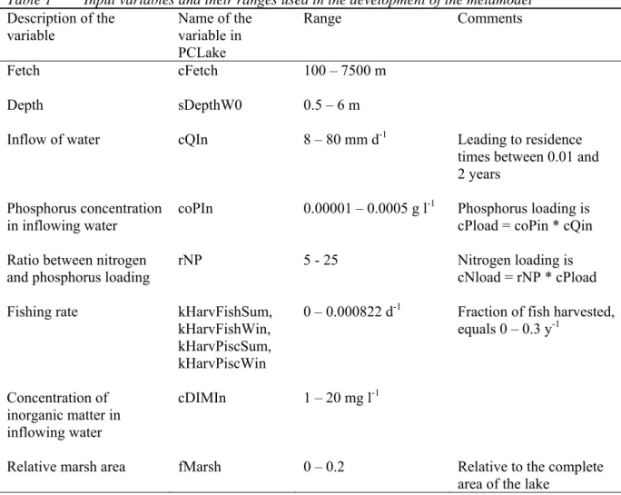
PCLake generates a large set of output variables. In this study metamodelling has been confined to simulation of the chlorophyll-A concentration in the water (mg m–3) during the summer after a period of 20 years. Each model run was executed with constant input values. In most cases, after 20 years, stabilisation of the simulated chlorophyll concentration had occurred. In developing the metamodel, variation in eight input variables was taken into account. The ranges of the input variables used in the study are given in Table 1. The ranges were determined with help of measured data from Portielje and Van der Molen (1998). The ranges do not only include present-day values but also possible future values that may be included in scenario studies with PCLake. Because of its mechanistic structure, PCLake can be used for simulations outside the range of input conditions that were used to estimate model parameters, more specifically to generate predictions for future conditions. The ranges of input variables used in this study imply that the metamodel may also be used for this purpose.

Table 1 Input variables and their ranges used in the development of the metamodel

Description of the variable Name of the variable in PCLake Range Comments Fetch cFetch 100 – 7500 m Depth sDepthW0 0.5 – 6 m

Inflow of water cQIn 8 – 80 mm d-1 _{Leading to residence}

times between 0.01 and 2 years

Phosphorus concentration in inflowing water

coPIn 0.00001 – 0.0005 g l-1 Phosphorus loading is cPload = coPin * cQin Ratio between nitrogen

and phosphorus loading

rNP 5 - 25 Nitrogen loading is

cNload = rNP * cPload Fishing rate kHarvFishSum,

kHarvFishWin, kHarvPiscSum, kHarvPiscWin

0 – 0.000822 d-1 Fraction of fish harvested, equals 0 – 0.3 y-1

Concentration of inorganic matter in inflowing water

cDIMIn 1 – 20 mg l-1

Relative marsh area fMarsh 0 – 0.2 Relative to the complete area of the lake

In the present version of the model, equal values are used for fishing rates of predatory and herbivorous fish species, in summer and in winter. Therefore, fishing rate was considered one single variable. In PCLake, the name of the output variable in PCLake, used for

2.2

Technical information

The computational costs of both PCLake and the metamodel are given for a PC with a 1.7 GHz Pentium 4 processor and 512 MB RAM. The operating system was Windows NT. On this system, the average execution time of PCLake, run in an ACSL Math 1.2

environment, was 9.0 seconds. Integration method was the second order Runga-Kutta-Fehlberg algorithm. The Math script used to run PCLake is given in Appendix 1.

2.3

Metamodelling techniques

In the study, three techniques were used to develop a metamodel for PCLake, (1) regression trees, (2) radial basis function networks in combination with regression trees, and (3) interpolation. Radial basis function networks (RBF networks) were chosen on the basis of Jin et al. (2000). In their comparative study of four metamodelling techniques – RBF networks, Polynomial Regression, Kriging Method, and Multivariate Adaptive Regression Splines – RBF networks gave the best results. The combination of RBF networks and regression trees was advocated by Orr (1999a). A regression tree was also used as a separate metamodel. As another alternative, interpolation was used because of its robustness.

2.3.1 Regression trees

The basic idea of a regression tree is to recursively partition the input space in two and approximate the function in each half by the average output value of the sample it contains. Each split is perpendicular to one of the axes so it can be expressed by an inequality

involving one of the input variables (xk > b, e.g. depth > 2.5). The input space is thus divided

into hyperrectangles organised into a binary tree. Each split is determined by the dimension (k) and boundary (b) which together maximally distinguish the response variable in the left and right branch, that is the split which minimises the residual square error between model and data over all possible choices of k and b. A disadvantage of the regression tree

metamodel is the discontinuity caused by the output jumping across the boundary between two hyperrectangles. To illustrate the principle, Figure 1 shows the chlorophyll concentration as a function of the phosphorus concentration of the inflowing water and the depth of the lake, as simulated by PCLake, and as approached by the regression tree model. In the

example, the chlorophyll values were calculated at fixed average values of the remaining six input variables.

When constructing a regression tree, it is to be decided when to stop growing the tree (or equivalently, how much to prune it after it has fully grown). Tree growing is controlled by two parameters, the node size at which the last split is performed (minsize), and the

minimum node deviance before growing stops (mindev). In this study, values of minsize=2

and mindev=0 were used. This implies that the tree was fitted perfectly to the data. In

statistical terms, this may not be the optimal model (most probably, it is largely

overparameterised), but it was considered optimal for the practical purpose of this study.

2.3.2 RBF networks

RBF networks are described by Orr (1996, 1999a). Note that the term ‘network’ is equivalent to the term ‘model’ that is more often used by statisticians.

RBF networks are linear models. The general characteristic of linear models is that they are expressed as linear combinations of a set of fixed functions. These fixed functions are often

Figure 1 The chlorophyll concentration as a function of the depth of the lake and the phosphorus concentration of the inflowing water, as simulated by PCLake (a), and as estimated by the regression tree metamodel (b) and the RBF network (c).

a

b

called basis functions. A linear model f(x) composed of m basis functions, hj(x), with weights wj, takes the form:

x). ( x) ( 1 j m j jh w f

∑

RBF networks are a special class of linear models in that they are linear combinations of

radial basis functions. The characteristic feature of radial functions is their response

decreases (or increases) monotonically with distance from a central point. A typical radial function, often used in RBF networks, is the Gaussian:

. ) ( exp ) ( ₂ 2      ₋ − = r c x x h (2)

Parameters are the centre c and radius r of the function.

In developing an RBF network with use of the Gaussian function one should determine the number of basis functions needed, and the parameters which they contain, c and r. In this study, these questions were addressed by using regression trees. Essentially, each terminal node of the regression tree contributes one basis function to the RBF network, the centre and radius of which are determined by the position and size of the corresponding hyperrectangle. Thus the tree gives an initial estimate of the number, positions and sizes of all RBFs in the network. The nodes of the regression tree are used not to fix the RBF network, but to generate a set of RBFs from which the final network can be selected. The regression tree from which the RBFs are produced is also used to order selections such that certain candidate RBFs are allowed to enter the model before others. Thus, model complexity was not

controlled in the phase of tree generation but in the phase of RBF selection.

The exact procedure to derive a RBF network in conjunction with a regression tree is given by Orr (1999b), and can be summarised as follows. In the construction of the regression tree, nodes are split recursively until a node cannot be split without creating a child containing fewer samples than a given minimum, minmem, which is a parameter of the method. The

resulting regression tree contains a root node (the initial node), some nonterminal nodes (having children) and some terminal nodes (having no children). Each node is associated with a hyperrectangle of input space having a centre c and size s defined as:

)], ( min ) ( max [ 2 1 ik S i ik S i k x x c ∈ ∈ + = (3) and: )]. ( min ) ( max [ 2 1 ik S i ik S i k x x s ∈ ∈ − = (4)

Subscript k denotes that size and centre are given in dimension k. S denotes the subset of the training set that is contained by the hyperrectangle. To translate a hyperrectangle into a Gaussian RBF, its centre c is used as the RBF centre c, and its size s scaled by a parameter

scales is used as the RBF radius r. Parameter scales has the same value for all nodes and is

another parameter of the method, in addition to minmem. Traversing the tree from the root to

the smallest hyperrectangles at the terminal nodes, RBFs are considered for inclusion in the model using the Bayesian Information Criterion (BIC) as a selection criterion:

SSE. ) ( ) 1 ) ln( ( BIC γ γ − − + = p p p p (5)

SSE is the training set sum-squared-error, p is the number of patterns in the training set (the number of model executions that the metamodel will be based on) and γ is the effective number of parameters in the model. Orr (1999b) states that BIC gave the best results of four possible model selection parameters. As an example, Fig. 1 illustrates the results of the RBF network compared to the original simulations with PCLake and the approximation by the regression tree metamodel.

For each value of minmem a different tree is built, and each value of scales gives rise to a

separate set of RBFs from which to select the network. The values of both minmem and scales can have an effect on the performance of the method. Orr (1996b) states that it pays

to experiment with different combinations of trial values to try and find one which works well on a given data set. In this study, minmem values of 3, 4, and 5 were used, and scales

values of 2, 3, 4, 5, 6, 7, and 8. The number of networks built by the method is equal to the product of minmem and scales (i.e. 21). The winning network is the one with the lowest

value of BIC.

2.3.3 Interpolation

Interpolation refers to deriving the output value for a point in input space from the output values of directly neighbouring given points. The basic idea of data interpolation is straightforward and transparent. The distances between the data points should be small, however, to obtain good estimates, and therefore a large number of model executions has to be done before interpolation. In this study, the data were organised into a grid before

interpolation. We considered that when the data points are organised into a grid, one may adjust the number of values per input dimension to the sensitivity of model output to the input variable concerned. In this way, the information taken from a fixed number of model

executions may be maximised. We chose to use FAST analysis (Campolongo et al., 2000; Chan et al., 2000) to determine the model sensitivity to the input variables. FAST offers a sensitivity analysis method that is independent of any assumptions on the model structure. As a rule of thumb, FAST analysis used a minimum of 65 executions per factor. In this study, 2000 executions were used in the FAST analysis. The FAST total sensitivity index is an accurate measure of the effect of a factor on the model output, taking into account all interaction effects involving that factor. The number of values per grid axis was taken proportional to the FAST total sensitivity index for the variable on the axis. The model PCLake was executed for the resulting grid of variable values.

2.4

Criteria for the performance of the metamodels

2.4.1 Accuracy

Accuracy is the capability of the metamodel of predicting the response in the input space of interest. The goodness-of-fit obtained from the training data is not sufficient to assess the accuracy of newly predicted points. Therefore, in this study, accuracies were measured by using an independent set of 80,000 simulations by PCLake, the input variables of which were sampled by latin hypercube. Several metrics are used to express the goodness-of-fit of the metamodel; these are Rfit2, the average residual, and some percentiles characterising the

∑

∑

where yi,PCLake is the chlorophyll concentration calculated by PCLake in execution i, yi,metamodel

is the chlorophyll concentration calculated by the metamodel in execution i, and yi,PCLake is

the chlorophyll concentration calculated by PCLake, averaged over all 80,000 executions.

Rfit2 expresses how well the values calculated by PCLake and approached by the metamodel

fit in a 1:1-relationship. It deviates from R2 calculated by linear regression through simulated and approached data, which expresses how well the data fit on a straight line, irrespective of whether this is an 1:1 straight line.

In some metamodels the number of input variables was less than eight. The input variables not included in these metamodels were represented as fixed average values. Also these reduced metamodels were tested with the above set of 80,000 simulations. It should therefore be stressed that the effects of the variables were excluded from the metamodel, but not from the test set that the reduced metamodels was tested with.

2.4.2 Efficiency

The efficiency of the metamodel is expressed in both the time required for constructing the metamodel and for predicting the response for the set of 80,000 samples mentioned above.

2.5

Software used

The model PCLake was run in an ACSL Math 1.2 environment. Sampling and sensitivity analysis according to FAST were done with help of SimLab. SPlus was used to construct a regression tree. Matlab functions developed by Orr (1999b), in particular rbf_rt_1, were

used to generate an RBF network in combination with a regression tree. Interpolation was done with the standard Matlab function for interpolation in multidimensional space, interpn. Interpn is suitable for data interpolation when inputs are distributed over input space

according to a grid (table lookup). Both 'linear', 'cubic', 'spline' and 'nearest'

were used as interpolation methods within function interpn. The practical procedures when

constructing a regression tree with SPlus, an RBF network with Matlab, and performing interpolation with Matlab, function interpn are given in Appendix 1. For all methods, the

number of executions needed for constructing the metamodel was limited to 100,000, i.e. about 10 days of calculations with PCLake.

3.

Results and discussion

Output values in the set that was used to test the metamodels ranged from 0.30 to 538.11 mg m-3. Mean output value of the 80,000 executions was 69.22 mg m–3. The frequency distribution of the simulated values is shown in Figuur 2. Frequency was

calculated as the fraction of output values per unit chlorophyll concentration (m3 mg–1). For practical reasons, in Figure 2, the X-axis was cut off at 200 mg m–3.

Figure 2 Frequency distribution of the PCLake output in the 80,000 runs test set.

3.1

Regression tree

In order to base the regression tree and the interpolation on equal numbers of model executions, 78,336 model executions were used for the construction of the regression tree (see 3.3). The resulting metamodel gave an Rfit2 of 0.884. A regression tree was also

constructed using only five variables, i.e. the depth, the fetch, the water inflow, the

phosphorus concentration, and the ratio between the nitrogen and phosphorus concentration. These variables were selected since they caused the greatest average difference between the chlorophyll values at their minimum and maximum values. Rfit2 of this metamodel was 0.911.

3.2

RBF networks

By experience it was established that the most extended data set containing the eight input variables given in Table 1, that can be processed by Matlab function rbf_rt_1, contains

5000 executions. When processing 6000 executions, the computer ran out of memory. According to the fit criterion produced by rbf_rt_1, the metamodel with minmem=3 and scales=3 gave the best fit to the training set. The resulting metamodel contains 393 centres.

The metamodel was tested with the test set of 80,000 points. The value of Rfit2 was 0.922.

When processing the test set by the RBF network, it had to be split into two parts because of computer memory restrictions. All 21 metamodels generated by rbf_rt_1 , corresponding to

the 21 combinations of minmem and scales, were tested with the independent test set. The

metamodel selected by the fit criterion in MatLab (minmem=3 and scales=3), also appeared

to be the best one when tested with the test set. 0 0.001 0.002 0.003 0.004 0 50 100 150 200 chlorophyll concentration frequency

In addition, an RBF network containing five variables, viz. the depth, the fetch, the water inflow, the phosphorus concentration, and the ratio between the nitrogen and phosphorus concentration, was constructed. These factors were selected using the same criteria as with regression trees. The network was based on 7000 executions, which was found to be the upper limit because of the available computer memory. According to the fit criterion

produced by rbf_rt_1, the metamodel with minmem=3 and scales=3 gave the best fit to the

training set. Testing the metamodel with the test set of 80,000 points produced an Rfit2 value

of 0.935.

3.3

Interpolation

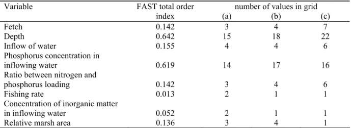
Results of the FAST analysis, that was used to assess the effects of the different variables on the output of PCLake, are shown in Table 2.

Table 2 FAST first order and total order indices for the variables in the model. Output variable was the summer chlorophyll-A concentration after 20 years.

The number of values for each variable in three grids: (a) based on FAST under the precondition that the number of values of each variable is ≥ 2, (b) based on FAST without restrictions; (c) using a more intuitive re-adjustment of the values calculated with help of FAST.

number of values in grid

Variable FAST total order

index (a) (b) (c) Fetch 0.142 3 4 7 Depth 0.642 15 18 22 Inflow of water 0.155 4 4 6 Phosphorus concentration in inflowing water 0.619 14 17 16

Ratio between nitrogen and

phosphorus loading 0.142 3 4 6

Fishing rate 0.013 2 1 1

Concentration of inorganic matter

in inflowing water 0.052 2 1 1

Relative marsh area 0.136 3 4 1

The total order indices were used to distribute the values of the variables at which the model is executed over the different axes. In calculating the number of values of the variables in the grid, the number of executions was determined at about 100,000. The numbers of values per axis were taken proportional to the FAST indices. In the first case, the distribution was calculated under the restriction that the number of values for each variable was ≥ 2 (Table 2, (a)). In the second case, no restriction was applied (Table 2, (b)). The third

distribution was a more intuitive re-adjustment of the numbers calculated on the basis of the FAST indices (Table 2, (c)). The actual resulting numbers of executions were

3 × 15 × 4 × 14 × 3 × 2 × 2 × 3 = 90720, 4 × 18 × 4 × 17 × 4 × 1 × 1 × 4 = 78336, and

7 × 22 × 6 × 16 × 6 × 1 × 1 × 1 = 88,704. Distributions of values over the axes were such that the two extremes of the axis were included and values in between were uniformly spaced. For the variables that had only one value, the value in the middle of the range was chosen. The fact that some variables were represented by the mean value of their range only, effectively reduced the number of variables in the metamodel compared to the original model.

The test set of 80,000 points to be estimated by interpn had to be processed in two parts

used as interpolation methods. With the available computer memory, method 'spline' could

not be used with a grid of this size.

Computational costs of the interpolation were 1.5 minutes, 10 minutes, and 2 seconds for methods 'linear', 'cubic' and 'nearest', respectively. Values of Rfit2 in grid (a) were

0.885 for method 'linear', and 0.766 for method 'nearest'. In this grid, method cubic

could not be used in this grid since it requires at least 3 values per axis. Values of Rfit2 in

grid (b) were 0.933, 0.929, and 0.827, for the three methods, respectively. In both cases, method 'linear' gave the best results. In grid (c), only interpn method 'linear' was

used. The resulting value of Rfit2 was 0.965.

3.4

Comparison of the metamodels

3.4.1 Accuracy

Accuracies of the metamodels containing all eight input variables are summarised in Table 3. Absolute values of the residuals were taken before percentiles were calculated. Interpolation was done with option 'linear' of the interpolation function interpn.

Table 3 Accuracies of the different metamodels, applied to the independent test set of 80,000 executions. The numbers between brackets in the column ‘technique’ indicate the number of variables included in the metamodel.

Technique Rfit2 mean

residual

Percentiles of the distribution of residuals

0.5 0.9 0.95 0.99 0.999

Regression tree (8) 0.884 10.03 6.32 21.64 31.69 66.00 130.69 RBF network (8) 0.922 8.29 5.26 17.57 25.95 54.34 114.99 Interpolation (8) 0.885 8.31 4.02 18.39 29.97 70.95 156.31

According to all criteria, the RBF network was the superior metamodel. The numbers of executions that the metamodels were based on, were 78,336 for the regression tree, 5,000 for the RBF network, and 90,720 for the interpolation. This indicates that the RBF network makes very efficient use of the available information. A difference between the models is that the RBF network may generate negative values for the chlorophyll concentration, whereas negative output values do not occur when using regression trees and interpolation. If desired, generation of negative values by RBF networks may be avoided by transformation (e.g. log-transformation) of the dependent variable.

Accuracies of the metamodels based on less than eight input variables, are given in Table 4. Note that testing the metamodels did involve all eight variables. Regression tree and RBF network were constructed using five variables. Interpolation was done with the grids given in Table 2(b) and 2(c), implying that both six and five variables were included in the

metamodel.

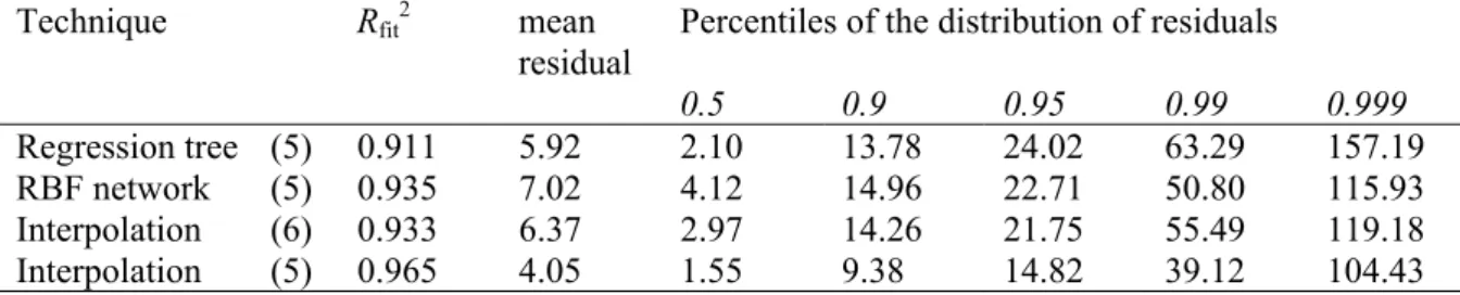
Table 4 Accuracies of different reduced metamodels, applied to the independent test set of 80,000 executions. The numbers between brackets in the column ‘technique’ indicate the number of input variables included in the metamodel.

Technique Rfit2 mean

residual

Percentiles of the distribution of residuals

0.5 0.9 0.95 0.99 0.999

Regression tree (5) 0.911 5.92 2.10 13.78 24.02 63.29 157.19 RBF network (5) 0.935 7.02 4.12 14.96 22.71 50.80 115.93 Interpolation (6) 0.933 6.37 2.97 14.26 21.75 55.49 119.18 Interpolation (5) 0.965 4.05 1.55 9.38 14.82 39.12 104.43

At a fixed number of model executions to construct a metamodel with, exclusion of less influential variables makes that the information on more influential variables can be increased on the expense of information on less influential factors. In the case of RBF networks, the number of model executions used to construct the network, that is limited by computer memory, can be increased. In both cases, the net effect is that the set of model executions used for metamodelling contains more information on the response of the dependent variable. This is reflected in the accuracies in Table 4, that are higher than those in Table 3, all across the line. Disadvantage of the metamodels in Table 4 is that variation in the variables that are excluded has no effect on the model result any more.

The results of interpolation in a 7 × 22 × 6 × 16 × 6 × 1 × 1 × 1 grid indicated that the grids that were constructed directly on the basis of FAST total order indices did not render optimal results in the interpolation. More than that, interpolation in a 7 × 22 × 6 × 16 × 6 × 1 × 1 × 1 grid was superior to all other metamodelling techniques used. The results of this metamodel are shown in Figure 3.

Figure 3 Output values of the best fitting metamodel as a function of PCLake output.

The fact that this metamodel was not made according to a prescribed algorithm implies that this is most probably not the optimal metamodel. When constructing a grid for interpolation with interpn, the importance of each variable can be expressed on a continuous scale, as the

number of values of the variable in the grid. When constructing a regression tree or an RBF network, one can only choose for either including a variable or not. The question that remains after this study is how to devise a formal procedure to select the variables that lead to an optimal metamodel.

The numbers of executions that the metamodels were based on, were 78,336 for the regression tree, 7,000 for the RBF network, and 78,336 and 88,704 for both interpolation

0 100 200 300 400 500 600 0 100 200 300 400 500 600

ChlA PCLake output (mg m-3)

ChlA metamodel output (mg m

-3 )

metamodels, respectively. Again, this indicates that the RBF network makes very efficient use of the available information.

3.4.2 Efficiency

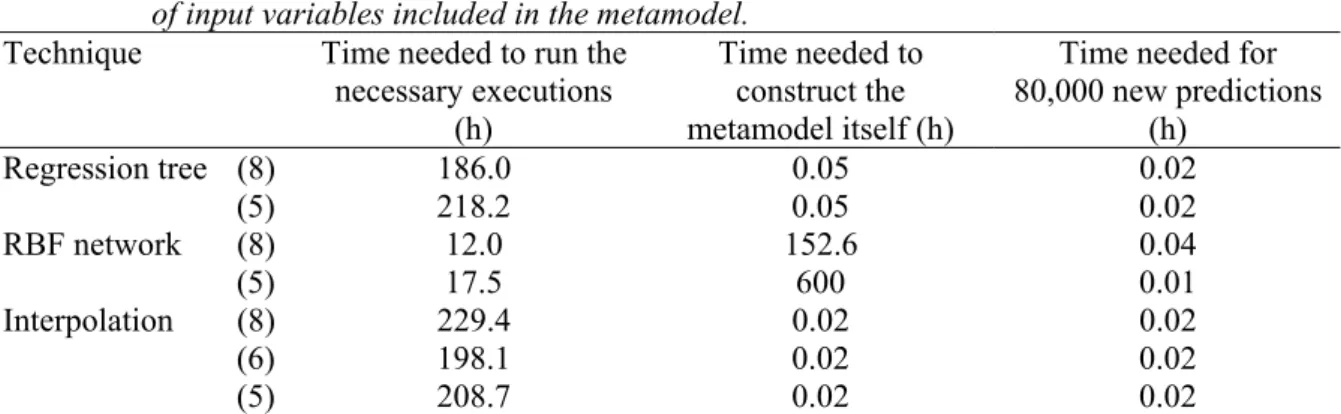
Efficiencies of the different metamodels are summarised in Table 5.

Table 5 Efficiencies of different metamodels, applied to the independent test set of 80,000

executions. The numbers between brackets in the column ‘technique’ indicate the number of input variables included in the metamodel.

Technique Time needed to run the necessary executions

(h)

Time needed to construct the metamodel itself (h)

Time needed for 80,000 new predictions (h) Regression tree (8) 186.0 0.05 0.02 (5) 218.2 0.05 0.02 RBF network (8) 12.0 152.6 0.04 (5) 17.5 600 0.01 Interpolation (8) 229.4 0.02 0.02 (6) 198.1 0.02 0.02 (5) 208.7 0.02 0.02

In all metamodels, the time needed to generate a result was reduced from an average duration of 9 seconds to 1 – 2 milliseconds. The overall time to develop the metamodel (i.e., running the necessary executions and constructing the metamodel itself) ranged from 7 – 9.5 days, exept for the RBF network with 5 variables and 7000 executions, which took about 25 days te be constructed. It may be more practical to reduce the number of executions used for this metamodel. This will probably slightly reduce the fit of the metamodel. In the metamodels using MatLab, i.e. RBF networks and interpolation, the test set of 80,000 predictions had to processed in two parts because of computer memory restrictions.

4.

Conclusions

Three methods (regression tree, RBF network, and interpolation) were used to develop a metamodel for the calculation of the chlorophyll concentration by PCLake. The best meta-model containing eight variables was the RBF network. R2 of the RBF network, using an independent test set, was 0.922. Constructing the metamodel on the basis of the five most influential input variables only (the depth, the fetch, the water inflow, the phosphorus concentration, and the ratio between the nitrogen and phosphorus concentration), improved the performance of the metamodel. The best metamodel containing five variables was that based on interpolation, giving an R2 _{of 0.965, using the same independent test set, (i.e. a set}

that contains the effects of all eight input variables on the output). The metamodel reduced computational cost from 9 seconds to 1-2 milliseconds. The metamodel may be used as a substitute for PCLake in scenario studies. No formal procedure was found that inevitably leads to the optimal conceivable metamodel. This implies that the R2 of 0.965 might be further improved, and that construction of future versions of the metamodel (e.g. for another output value of PCLake) may again involve some trial and error.

The practical procedures when constructing a regression tree with SPlus, an RBF network with Matlab, and performing interpolation with Matlab, function interpn are given

References

Campolongo F, Saltelli A, Sørensen T, Tarantola S. 2000. Hitchhiker’s guide to sensitivity analysis. In: Saltelli A, Chan K, Marian Scott E, eds. Sensitivity analysis. Chichester: John Wiley & Sons, 15-47.

Chan K, Tarantola S, Saltelli A. 2000. Variance-based methods. In: Saltelli A, Chan K, Marian Scott E, eds. Sensitivity analysis. Chichester: John Wiley & Sons, 167 – 197. Janse JH. 1997. A model of nutrient dynamics in shallow lakes in relation to multiple stable

states. Hydrobiologia 342/343: 1-8.

Janse JH, Van Liere L. 1995. PCLake, a modelling tool for the evaluation of lake restoration scenarios. Water Science and Technology 31: 371-374.

Jin R, Chen W, Simpson TW. 2000. Comparative studies of metamodeling techniques under multiple modeling criteria. AIAA Paper 2000-4801.

Orr MJL. 1996. Introduction to radial basis function networks. www.anc.ed.ac.uk/~mjo/papers/intro.ps

Orr MJL. 1999a. Recent advances in radial basis function networks. www.anc.ed.ac.uk/~mjo/papers/recad.ps

Orr MJL. 1999b. Matlab functions for radial basis function networks. www.anc.ed.ac.uk/~mjo/software/rbf2.zip

Portielje R, Van der Molen DT. 1998. Relaties tussen eutrofiëringsvariabelen en

systeemkenmerken van de Nederlandse meren en plassen. Deelrapport II voor de Vierde Eutrofiëringsenquête. RIZA rapport 98.007. Lelystad: RIZA.

Appendix 1 Procedures and scripts

In Appendix 1, procedures are given to construct a new version of the metamodel according to each of the three techniques.

1.1 Math script

The following Math script was used to execute PClake:

CQEVAVE=0.0 CQEVVAR=0.0 IALG=8 NSTP=200

!! set ECSITG = .T. !errors based on current value of state !! set TJNITG = 1.0D33 ! no messages on Jacobian nonlinearities !! output/clear !No screen output during run

!! set WESITG = .F. !No error summary after each run !! set WEDITG = .F. !No integration messages during run !!prepare time

!!prepare ochla !!prepare cpload !!prepare endyr

% The last year of the simulation is called ENDYR. endyr = ENDYR

ENDTIME = 365*ENDYR CPBACKLOAD = 0 CNBACKLOAD = 0

SaveInterval = 1000;

% Inputdata are read from file X_PCLake.txt. tablefilename = 'X_PCLake.txt'

readtable

parset = values

% nsamp is the number of executions nsamp = size(parset,1)

for isamp = 1:nsamp

CFETCH = parset(isamp,2) SDEPTHW0 = parset(isamp,3)

% The following parameters characterise the effects of wind on the processes in PCLake. CFUNTAUSETIM = ... exp(-exp((530.729/CFETCH+1.77903)+(-2694.65/CFETCH-0.412493)*SDEPTHW0)) CFUNTAUSETOM = CFUNTAUSETIM CFUNTAURESUS = ... 123.044 / (1+0.47991*exp((13.0811+0.0017092*CFETCH- 0.280058*sqrt(CFETCH))*SDEPTHW0))

KRESUSPHYTREF = 0.721617 * (1- exp (-0.378555*CFUNTAURESUS)) CQIN = parset(isamp,4)

COPIN = parset(isamp,5) CPLOAD = COPIN * CQIN

rNP = parset(isamp,6) CNLOAD = rNP*CPLOAD KHARVFISHSUM = parset(isamp,7) KHARVFISHWIN = KHARVFISHSUM KHARVPISCSUM = KHARVFISHSUM KHARVPISCWIN = KHARVFISHSUM CDIMIN = parset(isamp,8) FMARSH = parset(isamp,9) !!spare; start; spare

ochlasum20 = mean(_ochla(365*(endyr-1)+91:365*(endyr-1)+273)) result(isamp,1)=ochlasum20

% Save results every SaveInterval (=1000) runs:

if round(isamp/SaveInterval) == isamp/SaveInterval | isamp == nsamp save result @file='y_PCLake.txt' @format=ascii;

end end

1.2 Regression tree

SPlus Regression Tree

Importing data

Import file containing X-variables and corresponding y-variable, e.g. rtdata.txt. In this

study, the size of the file was 78,336 × 9. In SPlus, the Object is called rtdata.

Import file with X-values for which calculations by the metamodel should be made, e.g. rt_test_X.txt. In this study, the size of the test file was 80,000 × 8. In SPlus, the Object is called rt.test.X.

Constructing the metamodel

From the main menu choose Statistics > Tree > Tree Models. Tab ‘Model’:

In the window ‘Data’, fill in ‘rtdata’ under Data Set.

In the window ‘Fitting Options’, fill in:

Min No of Obs Before Split 1

Min Node Size 2

Min Node Deviance 0

In the window ‘Save Model Object’, fill in ‘rtmodel’.

In the window ‘Variables’, fill in:

Dependent ochlasum20

Independent select all X-variables.

Predictions with the metamodel

In Object Explorer, click on ‘rtmodel’ with the right mouse button.

Choose ‘Predict’.

In ‘New Data’, fill in ‘rt.test.X’.

In ‘Save As’, fill in ‘rt.pred’.

1.3 RBF network

Constructing an RBF network with MatLab functions developed by Orr, and using the network to make calculations are described in detail by Orr (1999b). The Matlab scripts can be downloaded from www.anc.ed.ac.uk/~mjo/software/rbf.zip and

www.anc.ed.ac.uk/~mjo/software/rbf2.zip.

A short summary of the procedure that was used is given here.

Construction of the RBF network

Import files with input data, e.g. rbfdata_X.txt (size 5000 × 8), and corresponding output

data, e.g. rbfdata_y.txt (size 5000 × 1).

Xt = rbfdata_X; y = rbfdata_y; X = Xt’; conf.minmem = 3 conf.scales = 2 [C, R, w, info] = rbf_rt_1(X, y, conf); info.dmc; infodmc = ans; info.rbf.gam; inforbfgam = ans; info.rbf.err; inforbferr = ans;

save rbfrt_3_2 C R w infodmc inforbfgam inforbferr;

The calculation may be repeated for other values of conf.minmem and conf.scales.

Predictions with the RBF network

Open workspace rbfrt_3_2.

Import file with points to be predicted, e.g. rbf_test_X.txt (size 80,000 × 8). A file of this

size should be processed in two parts. Here, the predictions are exported to drive c:\.

info.dmc = infodmc Xpred = rbf_test_X(1:40000,:); Xpredt = Xpred'; Ht = rbf_dm(Xpredt,C,R,info.dmc); yt = Ht * w; save('c:\rbfrt_ytest_3_2a.txt','yt','-ASCII') Xpred = rbf_test_X(40001:80000,:); Xpredt = Xpred'; Ht = rbf_dm(Xpredt,C,R,info.dmc); yt = Ht * w; save('c:\rbfrt_ytest_3_2b.txt','yt','-ASCII')

1.4 Interpolation

Matlab interpn

A. Import data

1. Import vector with outputs PCLake e.g. pclake_y.txt

2. Import file with inputs for which output should be estimated by interpolation e.g. interpn_test_X.txt

B. Command window

1. Rename output vector to y. e.g. y = pclake_y;

The number of elements of y is denoted ay.

In the example, ay = 78336.

2. Describe the grid of input values that were used to calculate y. Use function ndgrid.

[X1 X2 X3 X4 … Xx] = ndgrid(X1_min:X1_step:X1_max, X2_min:X2_step:X2_max, …, Xx_min:Xx_step:Xx_max);

Min denotes the minimum value of the variable, max denotes the maximum value of

the variable, step denotes the step size from min to max. The number of X-variables

is denoted x. The numbers of values per axis are a1, a2, a3, …, ax, respectively, for

variables X1, X2, X3, … Xx. e.g.

[X1 X2 X3 X4 X5 X6] =

ndgrid(100:2466.667:7500.001,0.5:0.32353:6.00001,8:24:80,0.00001:0.00 0030625:0.0005,5:6.67:25.01,0:0.0667:0.2001);

In the example, the numbers of X-variables are a1=4, a2=18, a3=4, a4=17, a5=4, a6=4.

3. Rearrange vector y into matrix B. A serves as an intermediate.

for i=1:(a_y/a₁),A=y(a₁*(i-1)+1:a₁*i,:);,B(i,1:a₁)=A';,end

e.g.

for i=1:19584, A=y(4*(i-1)+1:4*i,:);,B(i,1:4)=A';,end

4. Rearrange matrix B into the multidimensional matrix V. This is done by a nested for-loop with x-2 levels. In the x-2 for-for-loops, indices i3, i4, i5, …, i(x) are used. The symbols for the indices are chosen in order to obtain a logical structure of the statement.

for i(x)=1:a_x, for i(x-1)=1:a_x-1, for i(x-2)=1:a_x-2, …, for i4=1:a₄, for

i3=1:a₃, V(:,:,i3,i4, …,i(x-2),i(x-1),i(x)) = B(a₂*i3 + (a₂*a₃)*i4 + …

+ (a₂*a₃*a₄* … *a_x-2)*i(x-1) + (a₂*a₃*a₄* … a_x-2*a_x-1)*i(x) – (a₂ + (a₂*a₃) + (a₂*a₃*a₄) + … + (a₂*a₃*a₄* … *a_x-1) –1): a₂*i3 + (a₂*a₃)*i4 + … +

(a₂*a₃*a₄* … *a_x-2)*i(x-1) + (a₂*a₃*a₄* … a_x-2*a_x-1)*i(x) – ((a₂*a₃) + (a₂*a₃*a₄) + … + (a₂*a₃*a₄* … *a_x-1),:)’;, end, end, …, end

e.g.

for i6=1:4, for i5=1:4, for i4=1:17, for i3=1:4, V(:,:,i3,i4,i5,i6)=

B(18*i3+(18*4)*i4+(18*4*17)*i5+(18*4*17*4)*i6-

(18+18*4+18*4*17+18*4*17*4-1):18*i3+72*i4+1224*i5+4896*i6-(18*4+18*4*17+18*4*17*4),:)';, end, end, end, end

which evaluates to

B(18*i3+72*i4+1224*i5+4896*i6-6209:18*i3+72*i4+1224*i5+4896*i6-6192,:)';, end, end, end, end

5. Rename points to be estimated to matrix Y. e.g. Y = interpn_test_X;

Each row contains one point to be estimated, that is one value for each of the x variables.

6. Extract vectors Y1, Y2, … Yx from matrix Y. Each vector contains the values for one variable. Together, the nth elements of the vectors constitute one point to be estimated. e.g. Y1 = Y(:,1); Y2 = Y(:,2); Y3 = Y(:,3); Y4 = Y(:,4); Y5 = Y(:,5); Y6 = Y(:,6);

7. Interpolate. Estimated values are saved into vector VI.

VI = interpn(X1,X2,X3, … ,Xx,V,Y1,Y2,Y3, … ,Yx,method);

e.g.

VI = interpn(X1,X2,X3,X4,X5,X6,V,Y1,Y2,Y3,Y4,Y5,Y6,'linear');

FAST analysis was used for sensitivity analysis of the variables in the model. SimLab FAST analysis

A. Sampling

A short overview is given here. Sampling is described in detail in the SimLab 1.1 Reference Manual.

Statistical Pre Processor

New Sample Generation Configure

Select Input Factors

The first time when sampling from a set of variables, choose Create New. In this study,

uniform distributions were used for the input variables. Minimum and maximum values were set, according to Table 1.

Once the list is complete: Accept factors

The list of variables can be saved as a file with extension .fac.

Next time the same set of factors is used to take a sample from, the .fac file should be

opened first.

Select Method

Choose the settings that are relevant.

Give a name for the output file, the .sam file.

Generate generates the sample.

B. Sensitivity analysis according to FAST

1. Statistical Pre Processor

2. Model Execution

Configure (Monte Carlo) Select Model

deselect Execute external model

Output file: .txt: Save (replace if you are asked to do so)

OK

Start (Monte Carlo)

3. Statistical Post Processor

Analyse (UA/SA) OUTPUT VARIABLES

select the output variable(s), here ochlasum20 Add

New variable SA

Tabulated values: values of the first and total order indices

Chart Visualise

Factors

select all available factors (►)

OK

Pie chart was made