Contact: Arno Swart, RIVM
This is a publication of:
National Institute for Public Health and the Environment
P.O. Box 1 | 3720 BA Bilthoven The Netherlands
Page 2 of 5
1
Determination of the particle size distribution
1.1 Introduction
For development of dispersion modelling of micro-organisms and endotoxins, it is imperative to properly integrate the particle size distribution. Small and light particles may be transported over longer distances than bigger and heavier particles, since those more readily deposit on the surface due to gravity.
Further, the particle size distribution is an important aspect of the health impact of exposure to micro-organisms. Indeed, it is known that smaller particles may penetrate deeper into the respiratory tract where there is more opportunity for infecting the host.
For the purpose of dispersion modelling of emissions from farms, we need the particle size distribution at the point of emission from the farm. Far away from the farm environment the particles are subject to
processes that may alter their distribution, such as deposition. Hence we measure the particle size distribution in the stables. For this, we use the MOUDI sampler. Also we will consider the data collected in the study of Lai et al. (2014).
The atmospheric dispersion model OPS was not designed for micro-organisms and endotoxins, but rather for particulate matter (besides other compounds such as SO2, NOx and NH3), for which the total mass was reported, not the mass fractions in the size classes. Hence, we have extended the OPS model to keep track of the dust concentrations for the particle size classes separately. As a post processing we convert the dust concentrations to micro-organism concentrations by using the distribution of micro-organisms over the dust particle size classes. For this purpose, the dust samples obtained with the MOUDI, were also analysed for enumeration of micro-organisms using the PCR technique. For endotoxins, measurements were unfortunately deemed unrealiable, and those will not be further analysed.
1.2 MOUDI measurements
The measurements were performed using the MOUDI sampler. This instrument catches particles on a series of consecutive plates, in such a way that lighter particles tend to deposit on plates later in the chain. This is a process governed by probabilities. We developed a novel mathematical procedure, based on Bayesian inversion, which is able to produce continuous particle size distributions along with confidence bounds on the distribution. A technical exposition may be found in Appendix 9B.
The number of measurements was limited. We have three
measurements for layers, seven measurements for broilers, and one for both finisher pigs and sows. The distributions over particle sizes of grams of dust per m3, and the distribution over particle sizes of micro-organisms per gram of dust was determined. From this the distribution over particle sizes of the number of organisms per gram of dust may be
found. Note that with the PCR technique only DNA is measured, yielding bacterial loads for both alive and dead bacteria. We assume that the relative distribution of organisms over grams is the same for dead and living micro-organisms.
As mentioned before, the endotoxin measurements were unreliable, and we have taken a uniform distribution over particle sizes as an
alternative.
1.3 The Lai et al. (2014) study
In the Lai et al. (2014) study, particle size distributions have been determined for 13 different combinations of animal species / housing types. These were determined for two different housings, with two measurement days per housing. The distribution is reported discretised over 30 size classes in the range 0.25 – 32 µm. The sampling aparatus was the Grimm sampler, a portable aerosol spectrometer, which counts particles. The mass in size class i was determined using
𝑀𝑀𝑖𝑖=16 𝜋𝜋(𝑑𝑑𝑖𝑖10−3)3𝜌𝜌𝑖𝑖𝐹𝐹𝑖𝑖 ,
where Mi is the mass (mg/m3), di the width of the particle size interval (µm), ρi the density (mg mm-3), and Fi the number of particles per m3 as measured. Perfect spherical particles were assumed with an
aerodynamic density of 1 mg mm-3 (= 1000 kg m-3).
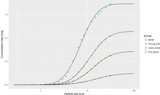
For the VGO modelling study, the authors provided us with the data set. The categories of animals did not correspond exactly, and we have made the following substitutions. For layer hen we substituted 'voliere', for finishing pigs we chose 'traditional', and for sows 'sow groups'. For the purpose of re-categorizing the 30 classes to the six classes used in OPS (Section 1.3), we fitted cummulative distributions of mass to the dataset, enforcing the the total mass implied by the fitted curves to be equal to the measured total mass (Figure 1). Given the fitted curves, it is straightforward to calculate the mass in any partition into discrete classes.
Page 4 of 5
The OPS atmospheric dispersion model
The OPS model makes use of a mass fraction distribution in six classes. The model calculates concentration and deposition for each of these six classes independently, taking into account differing properties of
particles in the different classes such as mass and size.
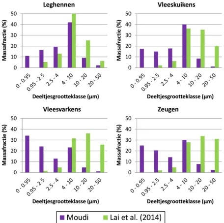
Figure 2 shows both the MOUDI and Lai et al. (2014) measurements in one figure. It is clear that large differences exist.
Figure 2. Mass fractions of dust in the OPS particle size classes, for each of the animal types. The colored bars indicate MOUDI measurements, or Lai et al. (2014) measurements – reclassified into the six OPS classes.
1.4 Discussion
As can be seen in Figure 2, the MOUDI and Lai et al. derived
distributions are not consistent. In the MOUDI measurements, most mass is found in the smaller size classes, while in the Lai et al. study hardly any mass was present there.
For the poultry data, there were quite a number of MOUDI measurents, and we do not believe that a small dataset is the cause of the
inconsistencies. At the moment a satisfying reason for the discrepancies is lacking.
The results of Lai et al. (2014) are more in line with other scientific literature and expert knowledge, and hence we chose to use the Lai data and not the MOUDI data for particle size distributions.
For the calculation of the numbers of micro-organisms per gram of dust in the several size classes, we do use the MOUDI measurements, since we have no reason to doubt the outcomes here.
For endotoxins a uniform distribution over the size classes was assumed, since the measurements were not deemed reliable.