Building Acoustics
Single-Leaf Walls
3
Airborne Sound Insulation of Single-Leaf Constructions
by L. Nederlof, J.J.M. Cauberg, L. Nijs and M.J. Tenpierik3.1
Introduction
It is quite common in practice to consider the airborne sound insulation as a construction property which will be or has already been measured, either in a laboratory or in a real-life situation. As far as measured data are available and reliable, it is highly recommended to use those. If such data are not available, measurements can still be done. In fact, sometimes you are obliged to do measurements.
However, measurements are costly and time-consuming which immediately raises the questions whether we can do without them. Besides, designing using an ever extending catalogue with typical constructions does not really seem smart. What we thus need is a physical model that predicts the sound insulation of a construction and shows the relationships between sound insulation, material, size and layout. Using such a model enables us to on the one hand predict the airborne sound insulation in advance and on the other hand design constructions more efficiently. In this chapter such a physical model for single-leaf constructions or in other words homogeneous constructions will be discussed.
3.2
Mass law for single-leaf walls
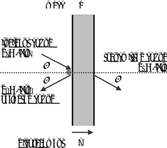
3.2.1 Theoretical mass law for normal incidenceThe sound insulation of a single-leaf wall can be theoretically predicted by a so-called mass law. Figure 3.1 schematically presents the acoustic model for airborne sound transmission through a homogeneous wall for normal incidence of sound waves. Coincidence effects, which will be discussed later in this chapter, can then thus be neglected. This model is a simplified version of reality since we assume that the wall has infinite dimensions in length and width. Besides, we assume that the wall consists of just one layer and is infinitely stiff so that no bending takes place (piston model). Moreover, we first assume normal incidence of sound waves. These simplifications allow a one-dimensional representation of the problem (Figure 3.1). When a sound wave reflects against a flat infinitely stiff construction, the following mathematical
relationship between the velocity of the acoustic waves and their respective pressures applies:
t u i r v v v t ∂ = = − ∂ pt ρair airc ut p pi r ∂ = = − ∂ (3.1a), with
vi = the vibration speed of air molecules of the incident sound wave [m/s]
vr = the vibration speed of air molecules of the reflected sound wave [m/s]
vt = the vibration speed of air molecules of the transmitted sound wave [m/s]
pi = the pressure of the incident sound wave [Pa]
pr = the pressure of the reflected sound wave [Pa]
pt = the pressure of the transmitted sound wave [Pa]
u = the displacement of the wall [m]
ρaircair = the specific acoustic impedance of a plane progressive wave (=410 kg/(m2∙s)).
On the incident side of the wall, the total sound pressure equals
i r
Figure 3.1 – Physical model for a single-leaf wall for normally incident acoustic waves.
Due to a pressure difference the wall starts to oscillate. According to Newton’s second law of motion the movement of the plate should then comply with
2 2 t u p p m t ∂ − = ∂ p p mt vtt ∂ − = ∂ (3.1c), with
m = the mass of the wall per square meter [kg/m2].
Combining equations (3.1a), (3.1b) and (3.1c) now yields the following differential equation
2 t i t air air m p p p c t ρ ∂ = + ∂ (3.2).
The general solution to this type of differential equation is such that, if pi is sinusoidal, pt is sinusoidal as
well and vice versa. If we now insert p pt = t;maxsin( )ωt in equation (3.2), we immediately see that this is indeed true: ω ω ω ω ω ω ρ ρ ρ = + = + ⋅ + 2
;maxsin( ) 2 ;maxcos( ) ;max 1 2 sin arctan 2
i t t t
air air air air air air
m m m
p p t p t p t
c c c (3.3),
with
ω = the angular frequency of the sound wave (ω = 2πf) [rad/s]
f = the frequency of the sound wave [Hz].
From equation (3.3) we directly observe that indeed pi is sinusoidal. The second term of the last sine-term
is the argument of the complex function and gives the phase shift of the transmitted acoustic wave relative to the incident sound wave. The square root term is the modulus of the complex function which is equal to the ratio of amplitudes of the incident sound wave to the transmitted sound wave
ω ρ = + 2 ;max ;max 1 2 i t air air p m p c (3.4). mass m incident sound pi = ρc·vi pr = ρc·vr reflected sound transmitted sound pt = ρc·vt p = pi + pr displacement u
Figure 3.2 – Physical model for a single-leaf wall for obliquely incident acoustic waves.
Sound intensity is directly proportional to the effective sound pressure squared and thus also with the amplitude squared of the effective sound pressure sincepeff =pmax/ 2for a sinusoidal sound wave. Using the definition of sound insulation, i.e. R=10log(1/t)=10log(Ii/It)=10log(|pi2|/|pt2|), we can now write for
the airborne sound insulation of a single-leaf homogeneous wall for normal incidence of sound waves
2 single; 10log 1 2
air air m R c ω ρ ⊥ = + (3.5).
3.2.2 Theoretical mass law for oblique incidence
Oblique incidence of sound waves can be treated in a similar way as normal incidence by using the components of vi, vr and vt along the normal of the construction in equations (3.1a) to (3.1c), i.e. by
multiplying the velocities with cosθ. This is shown in Figure 3.2. Equation (3.5a) then changes to 2
single; 10log 1 2 cos
air air m R c θ ω θ ρ = +
theoretical mass law (3.6a).
If ωm/2ρaircair >> 1, or in other words if fm >> ρaircair/π =130 kg/(m2s), this equation can be simplified.
Since in general we work with frequencies higher than 63 Hz, this condition is satisfied if m >> 2 kg/m2
which almost always is the case in practice except when thin foils or membranes are used. The simplified equation then becomes
single; 20log 2 cos 20log 500cos 12
air air m fm R c θ ω θ θ ρ ≈ ≈ +
theoretical mass law (3.6b).
These equations clearly demonstrate that according to the mass law the airborne sound insulation of a single-leaf wall increases with 20 log ω = 6 dB per octave (=6 dB per doubling of frequency) but also with 6 dB per doubling of mass; and that the highest sound insulation is found for normal incidence. So, the bigger the angle θ is, the worse the airborne sound insulation is. A practical consequence of this phenomenon can be observed in high-rise buildings where people on the highest floors sometimes experience more nuisance than on the lower floors. mass m incident sound pi = ρc·vi pr = ρc·vr reflected sound transmitted sound pt = ρc·vt θ displacement u θ θ
3.2.3 Theoretical mass law for random incidence
In practice, however, especially inside buildings, the sound field is diffuse. As a consequence, acoustic waves hitting the cavity construction have multiple directions. We assume that all directions, thus all angles of incidence, are equally and simultaneously present in the sound field in front of the construction. We call this type of incidence random incidence or uniformly distributed incidence. To obtain the airborne sound insulation for such random incidence, we must average equation (3.6b) over all angles of incidence1
within half a unit sphere. This is done as follows:
/2 /2
2 2
0 0
1 1
10log cos 10log 2 sin cos 5
2 d 2 d π π θ π θ θ θ π π Ω = ≈
∫
∫
(3.7).The airborne sound insulation of a single leaf wall for random incidence thus equals its airborne sound insulation for normal incidence minus approximately 5 dB.
single random; single; 5
R ≈R ⊥− (3.8).
3.2.4 Empirical mass laws for random incidence
The theoretical mass law predicts an increase of 6 dB/oct. In practice however this increase is mostly limited to about 5 dB/oct. Moreover, contrary to theoretical predictions the insulation curve is mostly not smooth and the sound insulation values are generally somewhat lower than according to theoretical predictions. Because of these issues so-called empirical mass laws have been developed as well. As the theoretical mass law, empirical mass laws assume infinitely stiff walls. They were however derived from measurements in a laboratory. One such empirical mass law for random incidence is
( )
single random; 17.5log 17.5log 500f 3
R = m + +
empirical mass law (3.9a).
Some other empirical mass laws exist to predict the sound insulation at 500 Hz. To get the values at different frequencies 4 to 5 dB needs to be added (towards higher frequencies) or subtracted (towards lower frequencies). They are given as
( )
single random; ;500 13.3log 10
R = m for m < 200 kg/m2 empirical mass law (3.9b),
( )
single random; ;500 15log 4
R = m for m > 200 kg/m2 empirical mass law (3.9c),
3 single random; ;500 12 5.3
R = + m empirical mass law (3.9d).
3.2.5 General frequency-dependent behaviour
Some anomalies in the sound insulation curves can however not be explained by both the theoretical and the empirical mass laws. For the derivation of these laws several assumptions were made. One of those was that the wall or plate had infinite stiffness. This implies that no bending phenomena can occur and that the behaviour of the plate in in-plane direction is totally neglected. In reality however such bending phenomena do occur and they can decrease the airborne sound insulation profoundly. Two such
phenomena exist: plate resonances at very low frequencies and coincidence (at higher frequencies). These phenomena will be discussed in the next sections.
1 In existing literature not all angles of incidence are taken; mostly only from 0o to some angle between 80o and 90o.
Angles of incidence larger than 80o hardly ever occur.
Figure 3.3 – General frequency-dependent behaviour of single-leaf wall.
The general frequency-dependent behaviour of the sound insulation of a single-leaf wall including bending phenomena can now be depicted. Figure 3.3 shows this general behaviour. As can be seen, at very low frequencies plate resonances dominate the acoustic behaviour of a single-leaf wall. As will be discussed in the next section such plate resonances are hardly ever observable in practice. Above these resonances, mass law behaviour theoretically predicts an increase of 6 dB/oct. represented by a straight line in the figure. Around or above a certain frequency, called the coincidence frequency, coincidence reduces the sound insulation considerably.
3.3
Plate resonances at very low frequencies
The model presented in the previous sections assumed an infinitely stiff plate which moves frictionless. Such a model does not entirely represent reality since walls and floors are attached to other parts of the building. As a result their movement especially near their edges is restricted. A sound wave hitting a wall or a floor thus causes transversal bending waves inside this wall or floor. The amplitude of these waves depends among others on material, size, thickness and edge conditions. At certain frequencies plate resonances occur which influence the airborne sound insulation.
In general bending waves thus lead to a lower airborne sound insulation. The sound that is radiated from a vibrating plate to a room can be represented by a so-called radiation factor σ which reflects the efficiency
with which vibration energy is given off from a construction element to air. The radiation factor of a plate that vibrates in bending thus is less than one. The radiation factor is defined as the ratio of the sound power given off by a plate and the sound power that would be given off by an equally large infinitely stiff plate that moves frictionless with the same average vibration speed:
2 air air W c v S σ ρ = (3.10), With
W = the radiated sound power of a plate or wall [W] v = the average vibration speed of the plate or wall [m/s] S = the surface area of the wall [m2].
Since the range of the vibration factor is very wide, in practice mostly a logarithmic scale is used. In figures that represent this radiation factor therefore most often 10logσ in stead of just σ is found along the vertical axis. f [Hz] R [d B] coincidence fc;θ plate
resonances mass law
6 dB/oct. increase of
Figure 3.4 – Plate resonances with modes 1,1; 1,2, 2,1; and 2,2 (Martin, 2007).
Plate resonances inside a single-leaf plate are thus caused by bending waves inside this plate. In fact they are transversal standing waves inside the plate, similar to the standing waves of a piano string. They occur in the direction of the length and the width of the plate but also in form of two-dimensional resonances. As shown in Figure 3.4. The frequencies where such standing waves occur depend among other on the edge conditions of the plate. Several edge conditions can be distinguished:
• rigidly connected edges no displacement and rotation possible
• hinged or pinned connection no displacement possible; rotation allowed • free connection both displacement and rotation allowed.
In practice most connections can in some way or another be schematised with sufficient accuracy as hinged or pinned connections. For this type of edge connection, the resonance frequencies, fn,m [Hz], for
standing waves inside a plate can be calculated from
2 2 , 2 n m p p B n m f d l b π ρ = + (3.11), with
n, m = an integer representing the mode of vibration (n=1, 2, 3, …; m=1, 2, 3, …)
ρp = the density or specific mass of the plate, wall or floor [kg/m3]
dp = the thickness of the plate, wall or floor [m]
l = the length of the plate, wall or floor [m] b = the width of the plate, wall or floor [m]
B = the bending stiffness of the plate, wall or floor per meter [Nm].
Structural mechanics tells us that for a single-leaf homogeneous plate the bending stiffness B equals
3 12 p Ed B= (3.12), with
E = the materials Young’s modulus or modulus of elasticity [N/m2].
Combining equations (3.11) and (3.12) yields
2 2 2 2 , 2 12 0.45 n m p p L p E n m n m f d d c l b l b π ρ = + ≈ + (3.13), with
cL = the speed of a longitudinal wave through a material similar to cair for air (cL = √(E/ρp)) [m/s]
n m 0 1 2 3 0 6 26 58 1 18 24 43 75 2 71 77 97 129 3 160 166 186 218
Table 3.1 – Frequencies where plate resonances occur inside a glass sheet of 1.5x0.9 m2 with a thickness of 6 mm.
Table 3.1 presents some values of the resonance frequencies of a 6 mm thick glass sheet. Plate resonances however in practice hardly ever cause problems. First, the lowest frequencies where plate resonances occur are quite low, i.e. far below the frequencies which are generally considered relevant in architectural acoustics (63 Hz – 4 kHz). Below these lowest resonance frequencies the acoustic behaviour of the plate is determined by its bending stiffness. In that very low frequency region, the mass law is no longer applicable. But as already stated this frequency region is very low and therefore not relevant to architectural practice while at the same time the wavelengths needed to cause the plate to vibrate are very large. In practice therefore hardly ever problems arise from low frequency plate resonances. They can however be observed when a heavy lorry or bus is passing a wall with glazed windows. Second, the higher resonance frequencies (n>1; m>1) in practice also hardly ever cause problems. They are easily weakened by internal dampening and edge dampening, since high frequencies are more effectively dampened than low frequencies. Only in case of thin non-dampened plates used around vibrating machines plate resonances need special attention. Here, increasing the amount of dampening resolves the problems.
3.4
Coincidence
As already explained the mass law cannot entirely explain the complete acoustic behaviour of homogenous constructions. Two phenomena related to the bending of the construction element are not explained by this law. The phenomenon of plate resonances at low frequencies was explained in the previous section. The phenomenon of coincidence will be treated in this section.
The term coincidence is used to describe the acoustic behaviour of a homogeneous wall under influence of oblique and random incidence of sound waves for the situation that two bending waves inside the material run together, or, in other words, coincide. These two waves are a free transversal bending wave and a forced transversal bending wave inside the single-leaf wall.
Figure 3.5 shows in a magnified way how the surface of a plate is deformed by the consecutive wave fronts of an incident plane progressive wave with a certain angle of incidence. Because of the progressive
character of the incident sound wave a transversal bending wave is forced onto the plate having a speed equal to csurf.
If we now look at a fixed point on the surface of the wall, it looks as if at that point the plate is excited by a point load. From such a point free transversal bending waves in the plate will start propagating. These same bending waves emerge when a plate is hit by for instance by a hammer. A typical example from practice are the bending waves that occur in a floor resulting from a person walking on heels. But also a sound wave might cause such free transversal bending waves.
+ + + +
- -
- -
- -
θ propagation direction of sound wave λair cairλsurf = λair / sinθ
csurf = cair / sinθ
Figure 3.5 – The generation of a forced transversal bending wave in a plate by a plane progressive sound wave. These free bending waves move with a certain speed through the material depending on the mass of the plate or wall, its dynamic stiffness and the frequency. This speed is described by
3 2 4 4 2 12 ω π = = p B Ed B c f m m (3.14), with
B = the bending stiffness per meter of the plate [Nm2/m] described by equation (3.12)
m = the plate’s mass per square meter [kg/m2] ω = the angular frequency (=2πf) [rad/s].
A propagation speed like this only occurs in very thin plates. The theory used to derive this equation is therefore called the thin-plate-theory. In plates or walls thicker than a quarter wavelength, bending and shear simultaneously occur, as a result changing the propagation speed of the forced wave inside the material.
In the wall or plate thus two types of bending waves simultaneously occur, each having its own speed: a free and a forced bending wave. Coincidence now occurs when both waves progress with the same speed through the material and their resulting deformations run together. In that situation both waves coincide and amplify their amplitudes. As a result, a drastic decrease in airborne sound insulation value of the wall construction is to be expected. This was already shown in Figure 3.3.
Mathematically speaking, coincidence thus occurs if
sinθ = = air B surf c c c (3.15), with
Equation (3.15) can be re-written in such a way that the frequency where coincidence occurs can be determined. The coincidence frequency can thus be calculated from
2 2 ; 2 2 12 1 2 sin 2 / sin θ = π air θ = airπ ρ θ c p p c m c f B d E (3.16a),
which approximately equals
; 2 64000 sin θ ≈ θ c p L f d c (3.16b), with
ρp = the density or specific mass of the plate, wall or floor [kg/m3]
dp = the thickness of the plate, wall or floor [m]
E = the plate’s dynamic Young’s modulus [N/m2]
cL = the speed of a longitudinal wave through a material (cL = √(E/ρp)) [m/s].
This equation clearly shows us that no coincidence occurs for normal incidence of sound waves.
This equation clearly demonstrates that no coincidence occurs for normal incidence of sound waves since θ=0o
and as a result sinθ =0. Moreover the lowest frequency where coincidence occurs is for 90o incidence of sound
waves, i.e. sound waves propagate in the same direction as the wall or plate. This lowest frequency is called the threshold frequency for coincidence, fc;th. Below this frequency coincidence cannot occur as well. It is however
important to realise that this coincidence restriction represents a limit situation, as a result of which some effect of coincidence can already be found below this threshold.
This threshold frequency can easily be found from equation (3.16) by inserting 90o for θ. The threshold
frequency is therefore found where
; 64000 ≈ c th p L f d c (3.17).
For each material thus the product fc;th·dp is constant. Table 3.2 presents the threshold frequency of several
examples of homogeneous walls. As can be seen, thickness, density, and dynamic Young’s modulus determine this frequency. Particularly thick heavy-weight construction walls might cause problems in practice since their threshold frequency for coincidence is in the range relevant for speech or traffic noise.
The extent to which coincidence however influences the airborne sound insulation of a homogeneous wall depends on the ability of the wall to convert the energy in the bending waves to heat, or in other words its ability to dampen bending waves. This ability is expressed by a loss factor for bending waves, η. For each
frequency, this loss factor can be determined from the measured structural reverberation time of the construction, Ts, according to
2.2 η= ⋅Ts
f (3.18).
In this loss factor all dampening mechanisms are included:
• dampening of the bending waves in the material itself (friction losses); • (rigid) connections along the wall’s edges (edge losses);
dp [mm] ρp [kg/m3] E [N/m2] fc ;th [Hz]
steel plate 3.5 7800 210·109 3500
wood chip board 36 650 3·109 800
float glass 6 2500 70·109 2000
concrete 100 2000 20·109 200
Table 3.2 – Threshold frequency (rounded) of several examples of homogeneous walls or plates.
material η [-] material η [-]
steel 1·10-4 - 3·10-4 concrete 4·10-3 – 8·10-3
aluminium 1·10-4 gypsum 6·10-3
iron 2·10-4 - 6·10-4 cellular concrete 1·10-2
copper 2·10-3 brick 1·10-2 – 2·10-2
lead 1·10-2 dry sand 6·10-2 – 12·10-2
glass 0.6·10-3 - 2·10-3 asphalt 5·10-2 – 4·10-1
spruce 0.8·10-2 filth 0.6·10-1
oak wood 1·10-2 fibrous blankets 1·10-1
plywood 1.3·10-2 cork 1.3·10-1 – 1.7·10-1
Table 3.3 – Some values of the loss factor of various materials (or actually constructions) (martin, 2007). Because the loss factor includes all aforementioned losses, it is no material constant but a property of the entire wall construction including its connections and construction flaws. For a specific type of
construction, an averaged value might be used for calculations. A measured curve however will irrevocably reflect a large standard deviation in the results. As can be seen from table 3.3 the value of the loss factor η
is around one or two percent.
With this loss factor now the airborne sound insulation of a homogeneous wall near the coincidence frequency can be determined from
2 ; sin ; cos 10log 1 2 θ ω θ η ρ = + c gle c air air m R c (3.19), with
ωc;θ = the angular coincidence frequency (ωc;θ = 2π fc;θ) [rad/s].
Compared to the original theoretical mass law, the airborne sound insulation near coincidence thus drops with about 20 log η. If no dampening losses are present, i.e. if η = 0, the sound insulation even drops to 0
dB.
Figure 3.6 – Coincidence effect for 6 mm float glass for several angles of incidence (63 125 500 1k 2k 4k f [Hz] η=0.01). 80O R [d B] 0 250 8k 0O 30O 45O 20 40 60 80 fc;th
Figure 3.7 – Coincidence effect for 100 mm concrete for several angles of incidence (η=0.04).
Figures 3.6 present the theoretical sound insulation curves of 6 mm float glass with infinite width and length. The dip due to coincidence approximately amounts to about 20 log (0.01) = 40 dB. In case of smaller plates, also edge losses will play a role as a result of which η becomes higher and as a consequence the drop in sound insulation smaller. In figure 3.7 the theoretical sound insulation curve of 100 mm concrete with infinite dimensions is shown. The drop in sound insulation resulting from coincidence now occurs at lower frequencies and falls into the frequency range of traffic noise. Figures 3.6 and 3.7 should however not be misinterpreted: coincidence does not disappear with decreasing angle of incidence; it only shifts towards higher frequencies.
Moreover, one should not let oneself be put off by the fact that the theoretical sound insulation curve for oblique incidence with certain specified angle of incidence even gets higher than the theoretical curve for normal incidence (θ=0o) according to the mass law. In practice this is hardly ever observed. In practice we
most of the time have to deal with random incidence of sound waves. Since sound is then coming from multiple directions, a wide spectrum of coincidence frequencies and consequently coincidence dips in sound insulation can be found in the insulation curve. The measured sound insulation curve reflects the resulting effect of all these coincidences and is too a large degree determined by the weakest link: the combination of frequency and angle of incidence that meets the coincidence requirement.
The result is that the sound insulation curve for random incidence first reflects the behaviour of the mass law, then exhibits a plateau and starting from the threshold frequency finally increases with about 7.5 dB/octave. This increase is less rapid than reflected in Figures 3.6 and 3.7 showing 18 dB/octave.
In the next section first two theoretical models that predict the entire acoustic behaviour of homogeneous walls will be discussed. And in section 3.6 the so-called plateau method will be described that reflects the acoustic behaviour of homogeneous wall constructions for random incidence of sound waves as observed in practice, thus with an increase of 7.5 dB/octave above the threshold frequency.
f [Hz] 63 125 500 1k 80O R [d B] 20 40 60 80 0 250 0O 35O 45O fc;th
3.5
Advanced theoretical mass law models
More advanced theoretical models exist that predict the entire frequency-dependent airborne sound insulation of homogeneous constructions, thus including coincidence effects. One such model is derived in a similar way as the mass law from section 3.1 but then in a more elaborate form. Nederhof and Cauberg (2005) present the result of this derivation as
2 2 sin ; 2 ; cos 10log 1 1 (1 ) 2 θ θ ω θ η ω ρ ω = + − + gle air air c m R i i c (3.20), with:
i = the imaginary unit (i2 = -1)
Since this theoretical model results in an increase of sound insulation of 18 dB/octave above the
coincidence frequency (Figures 3.6 and 3.7), which does not reflect the increase observed in reality, Häupl (2008) presents a semi-empirical equation that more closely but not entirely resembles the behaviour observed in laboratory measurements. It is written as
sin ; 2 2 2 ; ; 2 cos 2 20log 1 1 1 2 θ θ θ ω θ ρ ω ω η ω ω = + − + air air gle c c m c R (3.21).
For very high frequencies, ω >> ωc;θ, this equation predicts an increase of 6 dB/octave and a sound
insulation value 6 dB lower than according to the theoretical mass law (eq. (3.6)).
Figures 3.8 and 3.9 show the theoretical prediction of the airborne sound insulation of a 6 mm glass sheet and 100 mm concrete according to equations (3.20) and (3.21) for 45o incidence. As can be seen clearly,
differences between both theoretical equations arise for frequencies higher than the coincidence frequency. Here equation (3.20) predicts a too rapid increase while equation (3.21) predicts a too slow increase. Therefore the so-called plateau method was developed which more accurately predicts the acoustic behaviour of homogeneous walls for random incidence of sound waves in octave bands. This model is explained in the next section.
Figure 3.8 – Theoretical airborne sound insulation of 6 mm float glass at 45o angle of incidence (η=0.004).
f [Hz] 63 125 500 1k 2k 4k R [d B] 0 250 8k eq. (3.6) 20 40 60 80 eq. (3.21) eq. (3.22) fc;th
Figure 3.9 – Theoretical airborne sound insulation of 100 mm concrete at 45o angle of incidence (η=0.007).
3.6
Plateau method
As already explained, the general airborne sound insulation of homogeneous walls is: • below the lowest eigenfrequency of the wall determined by its flexural stiffness;
• in a limited frequency range from the lowest eigenfrequency till somewhat below the threshold frequency for coincidence determined by the inertia of mass resulting in an increase of 5 to 6 dB/octave;
• above the threshold frequency for coincidence possibly determined by coincidence (for oblique and random incidence);
• far above the threshold frequency for coincidence increasing with 7 to 9 dB/octave.
The exact shape of the sound insulation curve is strongly influenced by plate resonances and coincidence. A complete mathematical model that includes all these aspects is very complex. Simplified models have been developed that can easily be used in practice. Although these models are highly stylised and simplified, conscious use allows a good comparison of homogeneous walls among one another. One such simplified model is the 3-step model of plateau model for stony materials. This model predicts the airborne sound insulation of stony materials for random incidence rather accurately. It is described below.
In this model the sound insulation curve is stylised as three straight lines: a line representing the mass law (A), a line representing a plateau caused by coincidence (B), and a line representing the sound insulation above the coincidence threshold frequency (C). In Figure 3.10 these lines are shown.
Figure 3.10 – Plateau method for predicting the sound insulation of stony homogeneous walls for random incidence. f [Hz] R [d B] plateau (B) fc;th (A) (C) raised plateau (B*) 6 dB/oct. 7.5 dB/oct. 1= c th; 2η f f ∆Rplateau f [Hz] 63 125 500 1k 2k 4k R [d B] 0 250 8k eq. (3.6) 20 40 60 80 eq. (3.22) fc;th 100 eq. (3.21)
The plateau in this figure ends at the threshold frequency for coincidence but starts already near
1= c th; 2η
f f (3.22).
Based upon this frequency and the threshold frequency for coincidence the three lines can now be determined. In the low frequency region (A), the theoretical mass law for random incidence applies:
sin ; 5 20log 2 5 20log 500 7
A gle air air m fm R R c ω ρ ⊥ = − ≈ − ≈ + (3.23a);
the plateau between the frequencies f1 and fc;th (B) can be found by inserting the frequency f1 for f in the
previous equation
( )
1 ;( )
sin ; 1 5 20log 500 7 20log 500c th 10log 2 7
B gle f m f m
R =R ⊥ f − ≈ + = + η +
(3.23b);
in the high frequency region (C), the sound insulation again rises but now with about 7.5 dB/oct according to: ; 25log C B c th f R R f = + (3.23c).
With increasing mass of the wall construction, the coincidence effect becomes less strong; for heavy walls the threshold frequency drops to below 500 Hz which corresponds to a wavelength in the order of 1 m. As a result, in case of walls with normal dimensions the coincidence effect becomes less important. When using the plateau method, it is therefore allowed for walls with a mass higher than 70 kg/m2 to increase
the plateau with a certain value. The permitted increase equals
20log 70
plateau m
R
∆ = (3.23d).
The new raised plateau, line (B*) in Figure 3.10, however should remain between the (extrapolated) lines A and C. As a result, the start and end frequency of the plateau slightly shift towards higher frequencies. It is important to realise that the plateau already starts below the threshold frequency although actual coincidence cannot yet occur here. However, bending waves do already have an effect in this region. Moreover, materials with low bending wave attenuation, i.e. low loss factor, exhibit a certain swing around the plateau as shown in Figure 3.11.
Figure 3.11 – Swing around the plateau for stony homogeneous materials with low loss factor. f [Hz] R [d B] fc;th 1= c th; 2η f f
The entire airborne sound insulation of stony walls for random incidence can now be estimated if
knowledge of the frequencies f1 and fc;th and the height of the plateau RB are known. The schematised sound
insulation graph can now easily be found using the following steps: 1.) Determine fc;th;
2.) Determine f1;
3.) Determine the height of the plateau RB and construct line (B);
4.) Draw line (A) starting from f1 with a slope of 6 dB/octave;
5.) Draw line (C) starting from fc;th with a slope of 7.5 dB/octave;
6.) Only if the mass of the wall is higher than 70 kg/m2, determine ∆Rplateau and construct a new
horizontal line (B*) ∆Rplateau above line (B). This new line (B*) then replaces line (B).
Although the plateau method is easy to use and gives a sufficiently accurate prediction of the sound insulation, it is important to realise that it has its limitations. These limitations are:
• the influence of low frequency plate resonances is neglected; • the influence of the dimensions of the plate is neglected;
• the influence of stiffening elements attached to the wall or plate are not considered;
• for thick plates (dp > λ/4), non standard bending waves occur which are not considered by the model.
Moreover, a comparison of the plateau method to actual laboratory measurements has shown that: • in case of lightweight soft plates, especially if the loss factor is low, the sound insulation curve is much
more whimsical than predicted by the plateau model;
• in case of heavy plates a plateau hardly occurs but rather an increase of the sound insulation with frequency with a certain slope.
3.7
Layered constructions
This text will be completed later.3.8
Stiffened constructions
This text will be completed later.3.9
Practical considerations
Read chapter 12 Applied Sound Insulation from the book ‘Building Physics’ by A.C. van der Linden. This text will be completed later.
3.10 Literature
Häupl, P. (2008), Bauphysik – Klima Wärme Feuchte Schall, Ernst und Sohn Verlag, Berlin, 547 pages. Martin, H.J. (2007), Geluidisolatie, lecture notes for the course Acoustics 7S510, Eindhoven University of
Technology, Eindhoven.
Nederlof, L. and Cauberg, J.J.M. (2005), “Luchtgeluidisolatie – Coincidentie-effect”, Kennisbank Bouwfysica Module A17, Stichting Kennisoverdracht Bouwfysica.