Downscaling drivers of global environmental change. Enabling use of global SRES scenarios at the national and grid levels

(1)

Netherlands Environmental Assessment Agency (MNP), P.O. Box 303, 3720 AH Bilthoven, the Netherlands; Tel: +31-30-274 274 5; Fax: +31-30-274 4479; www.mnp.nl/en

Report 550025001/2006

Downscaling drivers of global environmental change

Enabling use of global SRES scenarios at the national and grid levels

D.P. van Vuuren, P.L. Lucas, H.B.M. Hilderink

Contact:

Detlef P. van Vuuren KMD

detlef.van.vuuren@mnp.nl

This investigation has been performed within the framework of S/550025 Methods for Sustainability Analysis

(2)

Parts of this publication may be reproduced, on condition of acknowledgement: 'Netherlands Environmental Assessment Agency, the title of the publication and year of publication.'

(3)

Abstract

Downscaling drivers of global environmental change

Global environmental change scenarios typically distinguish between about 10-20 global regions. However, various studies need scenario information at a higher level of spatial detail. This paper presents a set of algorithms that aim to fill this gap by providing downscaled scenario data for population, GDP and emissions at the national and grid levels. The proposed methodology is based on external-input-based downscaling for population, convergence-based downscaling for GDP and emissions, and linear algorithms to go to grid levels. The algorithms are applied to the IPCC-SRES scenarios, where the results seem to provide a credible basis for global environmental change assessments.

Keywords:

(4)

(5)

Rapport in het kort

Schalen naar gedetailleerd niveau van mondiale milieuscenario’s

Mondiale milieuscenario’s worden typisch gemaakt met behulp van modellen met zo’n 10-20 mondiale regio’s als geografisch detailniveau. Studies die de informatie van deze scenario’s kunnen gebruiken hebben echter soms een groter detail nodig. Het gaat hierbij bijvoorbeeld om klimaatimpactstudies (vaak informatie op gridniveau) of analyse van klimaatbeleid op landenniveau. Dit rapport beschrijft een set van algoritmes die dit gat kunnen vullen door informatie over populatie, inkomen en emissies te schalen (downscaling) van het niveau van mondiale regio’s tot het niveau van individuele landen en een 0,5 x 0,5 grid. De methodologie is gebaseerd op een combinatie van downscaling algoritmes: externe input schaling voor populatie, convergentie-gebaseerd schalen voor inkomen en emissies en lineaire algoritmen om naar gridniveau te gaan. De methode wordt toegepast op de IPCC- SRES scenario’s. Het rapport laat zien dat de resultaten een geloofwaardige basis voor gedetailleerde studies kunnen zijn.

Trefwoorden:

(6)

(7)

1 Introduction

Interaction between human and environmental systems has become an important focal point of research of the last decades. An important aspect of this relationship is scale. As different phenomena take place at different spatial scales, the preferred spatial scale depends on the analysis undertaken. In the case of studies that look into long-term future changes of the global environment and/or its driving forces, the scale of large global regions is often the most useful level of analysis. Major global scenario studies, such as the scenarios in the Special Report on Emission Scenarios (Nakicenovic et al., 2000), the Global Environment Outlook (UNEP, 2002) and the Millennium Ecosystem Assessment (MA, 2005) are

developed using models that typically distinguish between 10 to 20 global regions. In fact, in both examples, the official reports actually reported on a small number of regions (4-6). Here, another compromise is made between detail, the ability to present information and the ability to provide consistency checks with other parts of the report. The aggregation scale is often chosen as a compromise: it contains sufficient detail to capture differences between different parts of the world and avoids the additional complexity of modelling at a more detailed scale level. Such complexities include the large number of possible interactions between the different geographical units, the need to deal with local processes and the need to include local policies.

However, with other applications, a finer scale may be preferable. For instance, when analysing specific international policy options (e.g. post-Kyoto climate policy) the national level might be a preferred scale of analysis given the fact that the interests of individual countries play a major role in international negotiations (see Den Elzen, 2005). Impact, vulnerability and adaptation studies may require even higher levels of detail, i.e. the sub-national level and/or the more detailed grid level (see, for example Arnell, 2004; Parry, 2004). The reason is that crucial parameters that determine actual impacts – such as land use patterns or altitudes – can vary across very short distances, resulting in a need for location-specific information.

The situation described above means that most global environmental scenarios, which are developed at the coarse scale of world regions, fail to meet the needs of a potential group of users of these scenarios. Given the coarse scale of current global integrated scenarios (and probably of those in the future), downscaling provides one possible tool for generating information at finer resolutions. The term “downscaling” is used here for any process in which coarse-scale data is disaggregated to a finer scale while ensuring consistency with the original data set. A good downscaling procedure needs to comply with several criteria, including: 1) consistency with existing local data (for the base year); 2) consistency with the

(10)

original source (the scenario data on the much coarser scale); 3) transparency; and 4) plausibility of the outcome. While this last criterion may sound obvious, not all existing methods comply with it. At the same time, it is often not possible to define unambiguously what is plausible or what is not.

One areas where downscaling is frequently discussed is climate change impact analysis. The TGICA (Task Group on Data and Scenario Support for Impact and Climate Assessment) is a special body of the Intergovernmental Panel on Climate Change (IPCC). It is responsible for coordinating data development for climate impact analysis (IPCC, 2004). The TGICA has asked research teams to provide downscaled scenario data about socio-economic indicators at the level of individual countries rather than aggregated regions. A helpful initial effort was made by Gaffin et al. (2004). In their publication and the pre-publication of their results on the Internet, they stated extensive caveats to their results. Nevertheless, Castles and

Henderson (2003) and Pitcher (2004) still questioned several results of their downscaling approach. The results of Gaffin et al. (2004) were already available at the CIESIN internet address in 2003 (which allowed people to use and access the data at that time). Note too that the review by Picher has not been published in open, peer-reviewed literature, but did serve as input for an IPCC TGICA meeting. We cite the document here as it provides a valuable analysis of the results of downscaling by Gaffin et al. (2004). However, we will summarise the criticism as part of our discussion of earlier downscaling attempts in section 2. This criticism led the TGICA board to conclude that improved downscaling procedures are required for socio-economic data (IPCC, 2004).

The purpose of this paper is twofold. Firstly, we provide generic algorithms and

methodologies – taking into account the criticisms of earlier attempts – which can be applied to other sets of global scenarios. Secondly, we describe the results of one application of these algorithms, i.e. a consistent set of downscaled data for the IPCC-SRES scenarios. The

algorithms are defined for three important driving forces of global environmental change: population size, economic growth and greenhouse gas (GHG) emissions. We use three levels of aggregation: 1) the original regional data, 2) the national level (for about 220 countries) and 3) a 0.5o by 0.5o grid level (population and income only). The algorithms are described in this paper and discussed along with samples from the downscaled dataset, while the full dataset can be downloaded from our website. Data can be downloaded from

http://www.mnp.nl/en/publications/2006/DownscalingDriversOfGlobalEnvironmentalChange Scenarios.html

(11)

2 General methods used for downscaling global

environmental change scenarios

2.1 Different types of downscaling

As mentioned in the introduction, the term “downscaling” is used for a wide range of different procedures. Some important aspects can be identified in the available literature on downscaling. First of all, information can be downscaled to one particular region, e.g. a particular country (Carter et al., 2004) which encompasses only a part of the original dataset. Alternatively, it can be downscaled to a set of units that, taken together, still encompass the total domain. A second important factor is the scale level itself, as downscaling can refer to anything: from global regions or countries to a grid level. A third factor is the nature of the information. In the case of the IPCC-SRES scenarios, this information may include either socio-economic data or climate data (see for instance Mearns et al., 2004). Finally, a fourth factor is the purpose of downscaling: are the results a final end-point, or is downscaling only used as an intermediate step, while results are still interpreted on the broader scale? The latter was, for instance, the case during the construction of the quantitative MA scenarios (see Alcamo et al., 2005), where regional information was downscaled to the country level only to facilitate the coupling of simulation models that use slightly different regional definitions.

These very different aspects give rise to a range of methods, which can be seen as a

continuum from very simple algorithms to more complex methodologies such as conditional modelling. The general rule is that if less information is available, simpler algorithms need to be used. Below, we briefly discuss some general downscaling methods.

Conditional modelling

Models that operate at a finer scale and that are conditional on results and/or assumptions with a coarser resolution are used as a relatively refined way of downscaling scenario data. Here, the conditions set to the fine-scale model form the means to downscale information which can include the scenario storyline (at the very least) or one or more quantitative results. Conditional modelling can be used only if there is sufficient information about the

downscaled indicators and their relationships to other parameters at the finer scale. In the case of the IPCC-SRES scenarios, the description of the storylines is helpful in inferring consistent assumptions at finer scales. Bollen (2004), for instance, used the macro-economic WorldScan model to downscale the original GDP data in the IPCC-SRES scenarios for the four IPCC regions to the 12 WorldScan regions by 1) making sure that the sum of more detailed regions still complied with the original 4 IPCC-SRES regions and 2) making

(12)

assumptions within the model (for trade policies, factor productivity growth, demographic parameters and saving rates) that were consistent with the storyline of the SRES scenarios. Another example of conditional modelling is formed by regional climate models (RCMs). Local climate change is influenced greatly by local features such as terrain, which cannot be represented in the global climate models because of their coarse resolution. At the same time, finer models are impractical for the global simulation of long periods of time. RCMs have therefore been developed with a much higher resolution, but they cover only a limited area and a shorter period of time. Much of the input for these models therefore come from the coarse-resolution climate models – and they provide consistent information at a more detailed level (see for example Hadley, 2006). Another example is the work of Carter et al. (2004), who used several models to create socio-economic, emission and environmental data consistent with the IPCC-SRES scenarios for Finland, using both the SRES storylines and outcomes of the global models as boundary conditions.

Conditional modelling is less applicable for downscaling global socio-economic data into a fully comprehensive set of country data (worldwide) given the lack of appropriate models. A more general disadvantage of conditional modelling as a downscaling method is the impaired transparency of model-based methods. Most of the algorithms discussed in the next section can be described in just a few pages. By contrast, with models, the reader is generally referred to extensive model documentation.

Clearly defined algorithms

The second method is downscaling on the basis of clearly defined algorithms. The main difference with conditional modelling is that these algorithms do not themselves provide a description of the subject at issue (as a detailed economic model does for the economy or a regional climate model for climate change); they provide only a statistical description of how coarse information is disaggregated. Still these tools may be complex as those sometimes used to downscale climate information (Wilby et al., 2004). In the case of socio-economic data, however, a lack of more refined information seems to call for much simpler algorithms (with greater transparency).

Three generic algorithms are considered in this paper:

1. Linear downscaling. This method of downscaling assumes that all elements within the unit have the same growth rates as the larger unit. This method is applicable in cases where the differences between the units at the finer scale are relatively small, and when there is no information available to distinguish between them. The method, however, can be flawed if finer-scale units diverge too much from the average values. 2. Convergence downscaling. An alternative to linear scaling is to assume convergence

(complete or partial) of the units to the regional average, making sure that the total outcome is attuned to the pathway of the larger unit. This assumption is especially

(13)

applicable to cases where there are large differences between units within a region in the base-year and where there is already (partial) convergence between the original regions. The rate of convergence can be influenced and can be only partial during the scenario period.

3. External-input-based downscaling. This method requires other finer-scale scenarios to be available and uses relative positions of the subunits within the larger unit as the basis for downscaling. For instance, the relative share of a country within its region in one scenario can be used to downscale another regional scenario to that particular country. An advantage of this method is that it can capture the future dynamics of different units if these are included in the scenario used for downscaling.

2.2 Earlier attempts to downscale IPCC-SRES

scenarios/drivers

At least two earlier studies have attempted to downscale IPCC-SRES scenario data from the four large global regions (for which they were developed) to the country and grid levels. Gaffin et al. (2004) downscaled population and GDP drivers, while Höhne and Ulhrich (2005) downscaled the GHG emissions.

The work of Gaffin et al. (2004) used algorithm 3 and algorithm 1 for the population data and algorithm 1 for total GDP levels. It should be noted that the authors already pointed out several limitations to their work (they specifically mentioned implausibly high growth rates for some developing countries and base-year issues). This criticism was repeated in an external review (Pitcher, 2004). In brief, the main shortcomings of the results of the Gaffin et al. (2004) methodology are as follows:

1. Algorithm 3 was applied before 2050 (for most scenarios based on the basis of age-groups), but could not be used after 2050 as no country-level scenarios were available at the time of the study. Instead algorithm 1 was used. The abrupt change in algorithm resulted in discontinuities in growth patterns after 2050 for the majority of 181

countries for which data is given (a discontinuity of more than 0.2% in the annual growth rate is found for about 120 countries). For instance, Russia’s population declines by 0.5% annually between 2045 and 2050 (this decline increases steadily in the decades before 2045), but this rate is reduced to only 0.2%.

2. For GDP, the linear algorithm results in “unacceptable results” (wording taken from Gaffin et al. (2004)) where there are very large differences between country levels within a region. Further in this article, we will show that if countries like South Korea and Singapore are assigned the average Asian growth rates, this results in extremely high income levels for both countries. For the A1 scenario, eight countries (Republic

(14)

of Korea, Reunion, Singapore, Brunei Darussalam, New Caledonia, Macao, French Polynesia and Hong Kong) were assigned a 2100 income level above 500,000 US$/capita – while the richest OECD country, Switzerland, is assigned an income level of 280,000 US$/capita (in 2000, the income level of Switzerland was at least twice that of these countries). Another example is the position of countries compared to the USA. In 2000, only 8 countries had income levels higher than the USA. While the OECD region continues to have the highest income level of all regions in the original data, the 2100 downscaling results show that 65 countries have a higher income than the USA, with 52 of these countries being non-OECD countries. By the same token, one can also argue that the method also results in excessive growth rates for other developing countries – but in a less extreme way – or in unreasonably low per capita incomes for other countries.

3. A final shortcoming is that income downscaling was applied to total GDP, and not to per capita income. As this is done independently from the population growth rates, this can lead to serious differences in per capita growth rates within a region, again easily leading to implausible results (excessive growth rates for some developing countries compared to the growth rates of developed countries in equal conditions). Some of the implausible per capita income results discussed in the previous section may in fact come from this “unlinking” of income and population.

Höhne and Ulhrich (2005) used algorithm 1 in their attempt to downscale GHG emissions. Their results are basically open to the criticism discussed under points 2 and 3 for the downscaling of GDP data (not repeated here; see also Den Elzen (2005)). Moreover, this study did not provide a consistent set of socio-economic and emissions data as downscaling was done directly on the basis of emissions data. Including information on population or income can make the downscaling method more plausible, but also allow for expressing data in relative terms such as per capita emissions or emission intensities.

(15)

3 Methodology applied in this paper

3.1 Overall description

The purpose of this paper is to provide a consistent set of downscaled data for the IPCC-SRES scenarios at the level of individual countries and at the grid level of 0.5 x 0.5 degrees, taking into account criticisms of earlier attempts. A selection was made of the three generic algorithms discussed above. An overall description of the methodologies used is provided in Table 3.1, while details are discussed in the subsequent sections. For population downscaling we took advantage, in general terms, of new, country-level scenario data of the UN to apply external-input-based downscaling, i.e. method 3. For the other two datasets – income and emission levels – we used the partial convergence method, i.e. method 2, for income per capita and technology (emission intensity) levels. The rate of convergence is based on the scenario storyline and the rate at the regional level. Partial, conditional convergence is a powerful tool in the downscaling of scenarios since many long-term scenarios (including the SRES scenarios) show some degree of convergence for many socio-economic variables. In fact, also the population scenarios implicitly assume some form of convergence: each of the external population scenarios used in downscaling show some degree of convergence in underlying birth and death rates, consistent with historical trends (Wilson, 2001).

It should be noted that the algorithms used in this paper have deliberately been kept simple as a good downscaling method needs to be transparent. We will discuss the most important limitations of the method in the discussion section.

3.2 IPCC-SRES scenarios

The IPCC-SRES scenarios consist of a set of storyline-based scenarios to describe both changes in major driving forces (population, economy, energy production and use) and the resulting emissions for all major greenhouse gases. The set of scenarios is based on two fundamental uncertainties (axes): 1) whether future development will be dominated by further globalisation or more regional emphasis and 2) whether economic development goals are given priority over environmental and social goals. The extremes along these two axes create four storylines known as A1 (globalisation and economic orientation), A2

(regionalisation and economic orientation), B1 (globalisation and environment/social focus) and B2 (regionalisation and environment/social focus).Recently, there have been some

(16)

criticisms of the consistency of the IPCC-SRES scenarios with more recent data and

scenarios. Van Vuuren and O'Neill (2006), however, showed that the IPCC-SRES scenarios are, in most cases, still up-to-date for most parameters. All IPCC-SRES scenarios show some level of partial convergence in their assumptions and results. In none of the scenarios,

however, is there full convergence for the four global regions described. Two of the four scenarios – A1 and B1 – deliberately emphasise convergence as a leading theme in their storyline. Consistent with this, the level of convergence in the per capita income levels is strongest. In the reported results, convergence is lowest in the A2 scenario (again consistent with the scenario storyline). For our downscaling, we chose a year outside the scenario period that is relatively near the scenario horizon for A1 and B1, and relatively far away for A2. On the basis of storyline and the consistency of country-level and regional results, we chose the following convergence years: 2150 for A1 and B1, 2250 for A2 and 2200 for B2. The choice of a convergence year beyond the time horizon of the scenario is justified by the fact that no full convergence is achieved at the regional level in any of the SRES scenarios. It should be noted that the convergence equations (described in section 5) need to be adapted slightly to allow for convergence within the time period of the scenario. In section 5, we will show that these assumptions lead to country results that seem to be consistent with the regional trends.

Table 3.1 Overall description of the methodology applied in this paper

17 world regions 224 countries Grid level (0.5o by 0.5o)

Population IMAGE 2.2 Downscaling on the basis

of existing national-scale UN World Population Prospects

Linear scaling from the national level on the basis of the 2000 population map

GDP IMAGE 2.2 Downscaling on the basis of partial convergence rule

Multiplication of the national GDP per capita data and the population map

GHG emissions IMAGE 2.2 For CO2 from energy and

industry: downscaling on the basis of IPAT equation, assuming partial convergence of emission intensity. For other sources: linear downscaling.

(17)

3.3 IMAGE 2.2 implementation of the IPCC-SRES scenarios

We used the 17-region implementation of the IPCC-SRES scenarios in the IMAGE 2.2 model as the starting point of our analysis (IMAGE-team, 2001). The IMAGE 2.2 regional numbers for population were directly based on the information provided by the SRES modelling teams (see IMAGE-team, 2001). Results from the WorldScan model (Bollen, 2004) were used for GDP. Energy and GHG emissions are based on the submodels of the IMAGE 2.2 model, but conform to the harmonisation criteria as indicated in the IPCC-SRES report.

3.4 Base year

For the different geographic scales different base year sources are used (see Table 3.2). The IMAGE 2.2 implementation of the SRES scenarios is based on base-year data for 1995, and values for 2000 are model projections. By now, base-year data have become available for the year 2000. These new (country-level) data were therefore used as the starting point for our downscaling exercise. In order to be consistent with both the new base-year country-level data and the original IPCC-SRES scenario data, a linear correction value was used that

ensures full consistency with the base-year data on the one hand and the scenario data in 2100 on the other hand. In other words, a scaling factor was used that starts with the ratio between historical data and scenario values at the regional level in the base year and converges towards 1 in 2100.

Table 3.2 Overall description of the base-year data

17 world regions 224 countries Grid level (0.5o by 0.5o)

Population IMAGE 2.2 Base-year data from

UN (2003)

Base-year data from CIESIN (2003) GDP IMAGE 2.2 Base-year data from

World Bank (2004) and UNSTAT (2005)

Base-year data on the basis of population map and country data

GHG emissions IMAGE 2.2 Base-year data from

(18)

(19)

4 Population

4.1 Rationale behind downscaling methods

The population represents an important driver of global environmental change, directly influencing the consumption of goods and emission levels. Population size and structure are the outcome of the three basic underlying processes of birth, death and migration (see e.g. Hilderink, 2000). The intertwinement of mortality reduction and – with some delay – the decline of fertility is known as the demographic transition. There is considerable variation between countries in the phasing of the demographic transition, though a strong tendency towards demographic convergence can be seen (Wilson, 2001). In most high-income

countries, the demographic transition has entered its final stage and the process of ageing will peak in the coming decades. In many low-income regions, on the other hand, countries are still in the transitional phase and fertility is declining, resulting in a relatively young age structure. The age profile of a population is one of the crucial factors in future population growth and represents a major reason for not applying linear downscaling to population projections. Fortunately, in the case of population, the existence of authoritative national-scale projections provides the option of external-input-based downscaling. The most useful projections for this purpose are the long-range population projections (up to 2300) published by the UN (2003). Using the relative size of countries in the UN projections makes it possible to downscale the IPCC-SRES scenarios, while capturing some of the important dynamics resulting from differences in the age profiles of different countries. Alternatively, one can also use the various age groups in the UN projection to break down the population scenarios by age (O'Neill et al., 2005). The latter does not lead to very different results for population size, but has the advantage of generating more information (age profiles). We have used both method to provide national population data, and both data sets can be obtained from the authors. For most countries, 2050 differences are only 1-2% of total population. In this paper, we concentrate on the numbers obtained from the simplest method (downscaling based on total population size).

Population data can be downscaled from the national level to the grid level using a linear downscaling algorithm (each grid cell within a country changes at the country’s rate of change). Alternatively, more refined methods can be considered that model future population distribution on the basis of fertility, mortality and migration processes and

micro-characteristics such as population densities and urbanisation (Gutmann, 2000; Hilderink, 2004). However, variations in the definition of urbanisation, in combination with the weak relationship between population density and urbanisation, still constitute an obstacle to

(20)

appropriate implementation (Hilderink, 2004). At this stage, therefore, the simple linear method was preferred (based on better transparency).

4.2 Base-year data

The most important data relating to historical and future population trends are provided by the UN World Population Prospects (2004), including the three population variants for low, medium and high fertility. The UN long-range projections (UN, 2003) are used to extend the time horizon to 2300. At the sub-national level, CIESIN (2003) provides population data at a more detailed level: population per 20 square kilometres for 1990 and 1995.

4.3 Method used for downscaling

The three variants of the UN long-range population projections are used for downscaling the regional population. The low variant is used for A1 and B1, the medium variant for B2 and the high variant for A2.

) / ( * C R R C Pop A A Pop = (1)

In this formula, Ac represents population data for the national-scale scenario (here, the UN

data), Ar is equal to the sum of the population data of all countries within the region (again

based on the UN data) and Popr, is the total population of the regional scenario (here the

regional IMAGE data). Grid-level data is generated by assuming a growth rate equal to the national level for all grid cells within that country.

4.4 Results

4.4.1 Downscaling to the national level

The method described in the previous section leads to a set of population projections that are an improvement on the previous work discussed in section 2. The main reason is that the problems with downscaling discontinuities are eliminated. It should be noted that the results of the downscaling exercise depend on the original IPCC-SRES scenarios. At the moment, these scenarios are not longer fully reflecting current insights into possible future

demographic trends (Van Vuuren and O'Neill, 2006). The same methodology, however, can also be used for other (more recent) population projections.

(21)

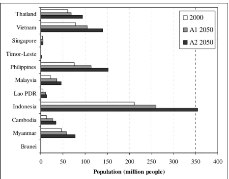
As an example of the results obtained, Figure 4.1 shows the results of the downscaling for the countries in the Southeast Asia region for the A1 and A2 scenarios. The Figure clearly shows the high population growth under the A2 scenario. In A1, the 2100 global population size is more or less equal to the current level while, in A2 in most countries, there is a doubling of the population. Figure 4.1 also illustrates that the external-input-based downscaling method can result in different growth rates for countries within a region.

0 50 100 150 200 250 300 350 400 Brunei Myanmar Cambodia Indonesia Lao PDR Malaysia Philippines Timor-Leste Singapore Vietnam Thailand

Population (million people)

2000 A1 2050 A2 2050

Figure 4.1 Absolute population numbers for South-East Asia in 2000, the base year, and 2050 for the A1 and A2 scenarios.

4.4.2 Downscaling to the grid level

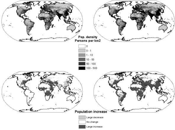
Figure 4.2 shows the grid level results for population density and population growth in the 2000-2100 period for the A1 and the A2 scenarios. The low fertility levels in A1 cause, in the long run, a fall in the population in the East Asia region, South Asia, the Former Soviet Union and Eastern Europe. In A2, on the other hand, where the continuing global population growth reaches approximately 15 billion people, almost all grid cells show a significant increase. The absolute population density maps in the two scenarios are less distinctive, but can provide a useful basis for many types of impact assessments.

(22)

Figure 4.2 Population density in 2100 for the A1 scenario (upper left) and A2 scenario (upper right), along with relative population growth between 1995 and 2100 for the A1b scenario (bottom left) and A2 scenario (bottom right)

(23)

5 Gross Domestic Product (GDP)

5.1 Rationale behind the downscaling method

Another important driver of global environmental change is the economic growth rate. In most scenarios, the economic growth rates of low-income regions are, on average, higher than those of high-income regions. This results in partial convergence of the income gap in relative terms. It should also be noted that, even in the case of partial convergence, this does not necessarily mean a reduction of the absolute income gap. The degree to which this partial convergence occurs, however, varies sharply across regions and scenarios. As stated earlier, the IPCC-SRES scenario set includes scenarios with a very high degree of convergence (A1 and B1) and scenarios with much less convergence (A2 and B2). Also scenarios exists in which some low-income regions will not experience higher growth rates than the global average, such as the World Bank/IMF projections for Sub-Saharan Africa (World Bank, 2005).

There is a very wide range of literature about whether income convergence is a logical attribute of larger economic systems and whether such convergence can actually be observed in the past. There is good evidence of convergence within large regions which act more or less as a common market (e.g. European Union, USA and Japan (Quah, 1996; Sala-i-Martin, 1996)). Similar evidence about convergence is found within groups of low-income countries, such as Western Africa (Jones, 2002). Whether convergence occurs globally is more

controversial, and also depends in part on the methodology used (compare Ben-David, 1996; compare Pritchett, 1997). Some form of convergence between regions seems evident, driven by much higher growth rates in Asia than the OECD (high-income) average. At the same time, Latin America and, in particular, Africa have yet not contributed to this convergence.

The fact that relative regional growth rates are often used as distinguishing factor between scenarios makes downscaling on the basis of convergence metrics attractive. This is reinforced by the fact that the evidence for intra-regional convergence is stronger than for inter-regional convergence. Convergence methods can avoid the major problem of

(24)

5.2 Base-year data

For the national per capita income levels in the base year, we used GDP per capita data from the World Bank’s World Development Indicators (WDI) measured in constant 1995US$ (World Bank, 2004). The data used are GDP per capita levels measured at market prices and translated into US$ on the basis of market exchange rates (MER). There has been discussion about the value of MER-based GDP estimates versus estimates based on purchasing-power-parity (PPP). MER numbers are used for this study, but the method can be applied equally well to PPP-based numbers. Since data is missing from this database for a small number of countries, we supplemented the set with GDP data from the UN Statistics Database

(UNSTAT, 2005). UN data is reported in 1990US$. Due to the lack of national inflation figures and a change in exchange-rate data for these specific countries, we used the consumer price index for the US from the WDI database (World Bank, 2004) to convert these constant 1990 prices into constant 1995 prices. Finally, as neither database reports income values for some of the small island states, we assumed the regional average income for these countries. For Taiwan (which is also not present in either dataset) where the per capita income level is much higher than in China, we used the Taiwan per capita income data from Young (1998).

5.3 Method used for downscaling

We assume partial convergence in per capita GDP for all countries within a region, using a convergence year (CY) outside the 2000-2100 time period, and 2000 as base year (BY). The downscaling consists of two steps. In the first step we determine a constant annual per capita income growth rate per country (GDPpc_grc) leading to the regional per capita income level

in the convergence year:

) ( 1 , , _ BY CY BY C CY R C GDPpc GDPpc gr GDPpc − ⎟ ⎟ ⎠ ⎞ ⎜ ⎜ ⎝ ⎛ = . (2)

In this formula, GDPpc refers to the per capita income. The indices C and R refer to the country and the region to which the country belongs respectively. As the GDP paths for the IPCC-SRES scenarios do not go beyond 2100, we extended the scenarios towards the convergence year using the growth rate in the last 10 years of the scenario run as a constant growth rate after 2100.In the SRES scenarios, most regions already have relative flat income growth rates during the last decades of the 21st century. It should also be noted that the corrections to make sure that the sum of country data equals the regional data (equation 6) imply that the method is insensitive to the assumed growth rate after 2100. The preliminary

(25)

per capita income of a country C at time step t (GDPpcC,t*) can then simply be determined by

multiplying the per capita income level of the previous time step by this constant growth rate.

C t C t C GDPpc GDPpc gr GDPpc* , = * ,−1* _ . (3)

Next, in the same time step, country-level per capita income is adjusted to make sure that the sum of total GDP of each country is equal to the regional total. This is necessary as the

regional growth rate changes over time (often starts high and decreases towards the end of the century). We first determine the difference between the regional GDP and the summed GDP of the individual countries (DiffR,t ):

t C c t C t R t R t R GDPpc POP GDPpc POP Diff _, = _, * _, −

∑

* , * _, . (4)

This difference term is attributed to the individual countries on the basis of their share in the increase of GDP in the region of that specific year (GDP_shC,t) (in other words, a country that

has a relatively large increase of GDP is assigned a larger share of the difference term):

∑

− − − − − − = CinR t C t C t C t C t C t C t C t C t C POP GDPpc POP GDPpc POP GDPpc POP GDPpc sh GDP 1 , 1 , * , , * 1 , 1 , * , , * , * * * * _ . (5)

The final per capita income (GDPpcC,t) can then be determined as:

t C t C R t C t C POP sh GDP Diff GDPpc GDPpc , , , * , _ * + = . (6)

In this method, the convergence year can be chosen freely, which introduces some form of flexibility. An early convergence year obviously results in more dispersed growth rates within a region than a late convergence year (see also overall methodology section).

Grid-level data can now be obtained by simply combining the per capita income levels on a country scale with the gridded population maps as determined in chapter 4. This assumes that per capita income is spread evenly over the whole country.

(26)

5.4 Results

5.4.1 Country-level downscaling results

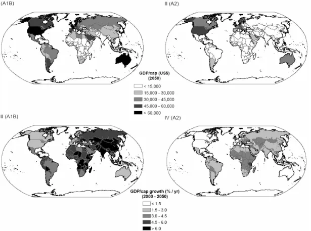
Figure 5.1 presents country-level per capita income levels in 2050 and the average annual growth rates for the 2000-2050 period for both the A1 and A2 scenarios. These economic indicators are not only relevant as outcomes of our downscaling methodology, but can also be used to judge the quality of the exercise. Criteria include the relative per capita income levels and growth rates (whether implausibly high growth rates are obtained). Figure 5.1 shows that, for 2050, the highest national per capita income levels in both scenarios are still found in current OECD countries. However, in A1, relatively high income levels are also found in several countries in South America, the Middle East and South-East Asia.

Figure 5.1 Per capita income in 2050 for the A1 scenario (upper left) and the A2 scenario (upper right,) and the annual per capita income growth between 2000 and 2050 for the A1 scenario (bottom left) and the A2 scenario (bottom right)

The A2 map, in contrast, is still a reasonable reflection of the current country levels for income. In terms of growth rates, a different picture emerges. Overall growth rates range from 2-8% annually in A1 and 1-6% annually in A2. The highest growth rates in both

(27)

and Latin America. The resulting growth rates seem to be within the range of growth rates found historically for different countries (World Bank, 2004) (although they are high for most developing countries as a result of the assumptions made within the IPCC-SRES scenarios themselves).

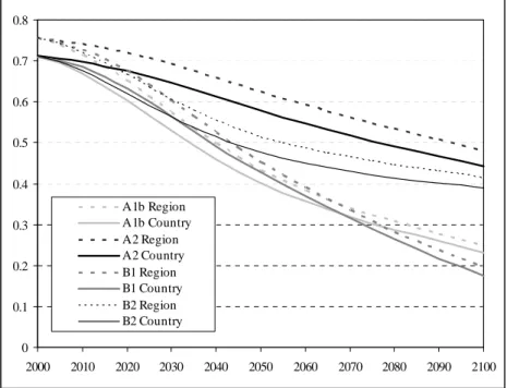
The level of difference in income levels across countries can be expressed by a global Gini coefficient. The Gini coefficient is a value between 0 and 1, where 0 corresponds to perfect equality (i.e. every country has the same income level) and 1 corresponds to total inequality (i.e. one country has all the income and others have zero income). Figure 5.2 shows the changes in the world’s Gini coefficient over time, based on the original regional income levels (before downscaling; dotted lines) and national income levels (after downscaling; straight lines). The original IPCC-SRES scenarios assume considerable convergence between the different regions. The downscaled data have a slightly higher level of divergence (as can be expected from the additional country detail) but reproduce the trends in the original regional scenarios very well, indicating that our downscaling methodology retains this element from the scenarios.

0 0.1 0.2 0.3 0.4 0.5 0.6 0.7 0.8 2000 2010 2020 2030 2040 2050 2060 2070 2080 2090 2100 A1b Region A1b Country A2 Region A2 Country B1 Region B1 Country B2 Region B2 Country

Figure 5.2 GINI coefficients for the world determined on the basis of regional data (original SRES) and downscaled country data

For a more in-depth analysis we focus on the results of the countries of the South-East Asia region. Given the very large initial income differences between the countries in this region (e.g. Singapore versus Vietnam), it is one of the regions where the critique related to the linear downscaling methodology is most pertinent. The left-hand graph in Figure 5.3 presents the per capita income growth rates of Singapore and Vietnam using the downscaling

(28)

methodology presented in this paper. The growth rates are presented in two steps. The flat lines indicate the annual growth rate that the countries need to follow (using equation 2) to reach equal per capita income levels in the convergence year (the convergence year is 2150 for this A1 scenario). The curved lines represent the final growth rates (equation 6), which have been adjusted to follow the intertemporal pattern of the regional growth rate (to ensure that, at each point in time, the sum of the GDP of all countries equals the regional GDP). The regional per capita GDP growth rate has a distinct pattern, starting from low numbers (as a result of the Asia crisis in the late 1990s) towards more than 5% a year in the first half of the century and levelling off to 2.5% a year in 2100. This pattern is well reflected in the growth rates of the two countries, but at a different level. Singapore stays well below the regional average growth rate and Vietnam needs a much higher growth to catch up with the rest of the region. The figure also shows that the growth rate of Vietnam after downscaling corresponds more or less to its historical growth rate. The growth rate for Singapore is lower than its historical growth rate – and is more consistent with those of high-income level economies (OECD). 0 20,000 40,000 60,000 80,000 100,000 120,000 140,000 160,000 180,000 200,000 2000 2020 2040 2060 2080 2100 P e r capi ta inc o m e ( U S $ /c a p ) 0 10 20 30 40 50 60 70 80 90 100 In c o m e d ispar it y (S in gapo re /V iet n a m ) Singapore Vietnam South-East Asia Income disparity -6.0 -4.0 -2.0 0.0 2.0 4.0 6.0 8.0 10.0 1990 2000 2010 2020 2030 2040 2050 2060 2070 2080 2090 2100 G row th r a te (% /y r) Singapore flat Vietnam flat Singapore corrected Vietnam corrected South-East Asia

Figure 5.3 Per capita income growth rates for the two calculation steps for Singapore and Vietnam (left) and per capita income and the income disparity between both countries (right)

It should be noted that the downscaled growth rates in several countries (not shown) are somewhat discontinuous with their historical growth rates. There are two factors that cause this. The main reason is that discontinuities already exist in the IPCC-SRES. This mainly holds for Central America and Africa, where several countries had negative growth rates in the 1990s, while the scenarios assume high growth rates in the first half of the 21st century. The second cause is the convergence rule. Countries with high income levels, like Singapore, are assumed to have lower growth rates in the future in order to converge to their regional levles. While future growth is obviously uncertain, this result could be interpreted as being consistent with economic theory. High growth rates in countries like Singapore may be more difficult to achieve in the future as result of reduced competitiveness (given their high labour

(29)

costs) and proximity to the technology frontier. Given these two factors and the fact that shifts in economic growth rates also occurred in the past, we do not believe that it is useful to introduce consistency with historical trends (at country level) as an additional requirement in our downscaling methodology at the costs of the transparency of the method.

The right-hand graph in Figure 5.3 shows the per capita income levels for Singapore and Vietnam compared to the regional average. The ratio between the income levels of both countries is also shown (right y-axis). In the base year, per capita income in Singapore is 75 times higher than that in Vietnam. After downscaling, the income level for Singapore in 2050 is around 100,000 US$ per capita, which is similar to the upper range of the OECD countries in 2050 (Luxemburg/Switzerland). This means that Singapore occupies an almost equal position relative to the OECD in 2000 and 2050. For Vietnam, the calculated income level in 2050 is around 10,000 US$ per capita. This is a decrease: from an income disparity compared to Singapore of a factor 75 to a factor 10. In 2100, the income disparity between both

countries has decreased further to a factor 2.

Table 5.1 Income per capita for the A1b scenario in 2050 determined using the method

2000 2050 Annual growth Earlier method This study Earlier method This study US$/cap US$/cap US$/cap %/yr %/yr

South-East Asia 1478 18336 18322 5.2% 5.2% Brunei 10786 97942 68470 4.5% 3.8% Myanmar 607 8356 12500 5.4% 6.2% Cambodia 388 3148 12160 4.3% 7.1% Indonesia 1015 13826 16550 5.4% 5.7% Lao PDR 451 3674 13187 4.3% 7.0% Malaysia 4808 51499 41796 4.9% 4.4% Philippines 1173 13057 19420 4.9% 5.8% Timor-Leste 176 1571 7497 4.5% 7.8% Singapore 28295 420580 93446 5.5% 2.4% Vietnam 370 4595 10032 5.2% 6.8% Thailand 2828 42289 27554 5.6% 4.7%

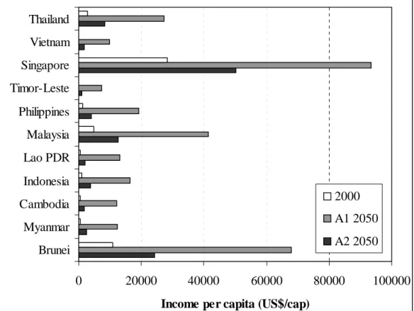
In a final analysis, we compare the results of the per capita income levels all countries in South-East Asia using the methodology applied by Gaffin et al. (2004) and the methodology presented in this paper (see Table 5.1; Figure 5.4). The earlier methodology differs in two ways from that applied in this paper: firstly, a linear downscaling algorithm was used and, secondly, GDP was downscaled rather than GDP per capita. We used the Gaffin et al. (2004)

(30)

methodology instead of reported results to eliminate influence of the base-year data. The results show that their methodology leads to high income levels for countries starting with a relatively large income share and a large regional growth rate. By contrast, the low-income countries in the same region remain relatively poor. This large difference results from the equal growth rates for all countries within the region, and is even aggravated by the fact that the population levels in low-income countries tend to grow faster than in higher-income countries. The results for the methodology presented in this paper seem to be more plausible: countries do not achieve improbably high income levels. Moreover, countries starting with a relatively large per capita income have lower income growth rates than countries starting with a relatively low per capita income. This is consistent with both the literature on

conditional convergence and the scenario storylines. At the same time, high-income countries still achieve much higher per capita income levels than the low-income countries. Den Elzen (2005) made a more detailed (worldwide) comparison between the two methodologies.

0 20000 40000 60000 80000 100000 Brunei Myanmar Cambodia Indonesia Lao PDR Malaysia Philippines Timor-Leste Singapore Vietnam Thailand

Income per capita (US$/cap)

2000 A1 2050 A2 2050

Figure 5.4 Per capita income for the countries of South-East Asia in 2000, the base year, and in 2050 for the A1 and A2 scenarios.

(31)

5.4.2 Downscaling to the grid level

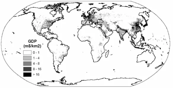
Figure 5.5 shows that the gridded GDP density ($/km2) values for the A1 scenario in the year 2050 follows largely the same patterns as the population maps. The highest GDP densities are found in Western and Central Europe, both coasts of the USA and Japan due to high per capita income levels and relatively high population densities. The GDP densities are also high in India, East Asia, and parts of South-East Asia due to intermediate per capita incomes and high population densities. Over time, there is an increase in density and a shift from the OECD regions to the Asian region with the highest values. These density levels are obviously relevant for impact analysis as they relate largely to consumption patterns and coping

capabilities.

In our current methodology we assume that income is evenly spread within countries. While differences between urban and rural areas may exists even in developed countries, these differences are likely to be more accentuated for developing countries. Using sub-national data to describe the current situation could be a major improvement (see Nordhaus, 2006; see Sachs et al., 2001), which was already acknowledged by Gaffin et al. (2004) but not applied in their work.. Furthermore, combining this set with a convergence methodology would also improve future projections.

(32)

(33)

6 Greenhouse gas emissions

6.1 Rationale behind downscaling method

Greenhouse gas (GHG) emissions are a function of socio-economic driving forces such as population and per capita income levels, but also of technological advances such as energy efficiency and the type of fuels used. Several simplified equations have been postulated to describe this interdependence, such as the IPAT equation (Ehrlich and Holdren, 1971) and the related Kaya identity (Kaya, 1989). The IPAT equation represents environmental impact (I) as the product of three indicators: population (P), affluence (A) and technology (T). Using GHG emissions for impact, per capita income levels for affluence and emission intensity (emissions per unit of GDP) for technology yields an identity equation that can be used to analyse trends in GHG emissions.

In our downscaling approach, we distinguish between six emission sources, i.e. 1) CO2,

2) CH4 and 3) N2O emissions from energy generation and industrial processes, 4) CH4 and

5) N2O emissions fromagricultural processes and total F gases (HFCs, PFCs and SF6). For all

energy and industry related emissions, the majority of emissions, we use the IPAT equation as the downscaling framework as these emissions are driven by population growth and income levels. Instead, simple linear downscaling is used for the other categories as they are only loosely linked to consumption (and much more to production). Finally, the CO2 land-use

change and forestry emissions have not been included since this would require some form of description of forest dynamics in our downscaling algorithms and this is an area to which we have not yet paid attention.

Population and per capita income levels were already downscaled in the previous two sections. Emission intensity generally decreases over time in most scenarios. As with per capita income levels, most scenarios – including IPCC-SRES – show partial convergence of emission intensities across regions over time. This convergence is driven by a spread of technologies, but also by maturing economies (i.e. agricultural advancing to post-industrial economies) all around the world. As emission intensities converge at the regional level, it makes sense, once again, to use a convergence algorithm for downscaling regional emission intensities.

(34)

6.2 Base-year data

Country data from the CAIT database (WRI, 2004) are used for greenhouse gas emissions. This database covers all GHG emissions, including energy generation, industrial processes, agricultural practices and waste, for all gases included in our methodology.

6.3 Method used for downscaling

For energy-related and industrial emissions, we use the IPAT relation to downscale the emission data to country level data (EC,t) using relative changes of the individual components

compared to base-year level:

0 , , 0 , , 0 , , 0 , , * * * C t C C t C C t C C t C EI EI GDPpc GDPpc POP POP E E = . (7)

The population and GDP data are already available. The convergence algorithms for

downscaling energy intensity are the same as for income (see equations in section 4.3), where per capita income, GDPpc, is replaced by emission intensity, EI (EIC,BY being the country’s

emission intensity in the base year and EIR,CY the emission intensity of the region in the

convergence year). ) ( 1 , , _ BY CY BY C CY R C EI EI gr EI − ⎟ ⎟ ⎠ ⎞ ⎜ ⎜ ⎝ ⎛ = . (8)

As with Formula 3, increases in emission intensity can be used to determine the preliminary emission intensity (EI*) and total emission levels (E*). As with income, we first determine the difference between the regional emission numbers and the sum of country emissions (calculated on the basis of equation 7; comparable to equation 4). Next, we assign this difference on the basis of the country’s share in total regional emissions:

∑

= CinR t C t C t C t C t C t C t C EI POP GDPpc EI POP GDPpc sh E _* , , , * , , , , * * * * _ . (9)

(35)

The final emission level (EC,,t) can then be determined as: t C R t C t C E EDiff E sh E _, = * , + * _ _, (10)

We use the same convergence year (equation 8) as in the per capita income downscaling for the different scenarios.

Finally, by contrast with the population and GDP downscaling, emission levels have not been scaled to the grid level. Work on historical emissions maps have been published earlier by Olivier and Berdowski (2001). These maps can easily be used as a basis for further

downscaling attempts in a similar way as that presented in section 5 for GDP. Scenario-based grid-level emission maps have been published earlier by Olivier et al. (2003).

6.4 Results

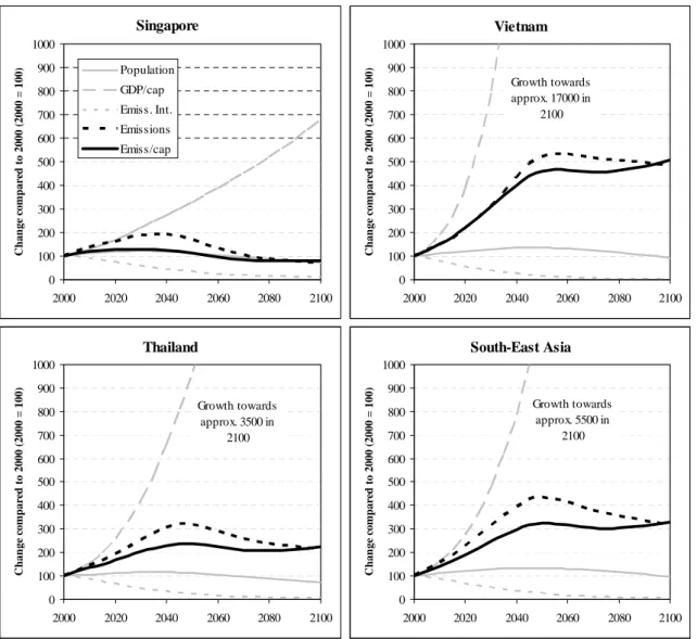
We will discuss the results of our downscaling method using again the South-East Asia region as example. Figure 6.1 shows how the downscaling results for emissions are obtained for Singapore, Vietnam and Thailand in the case of the A1 scenario.

(36)

South-East Asia 0 100 200 300 400 500 600 700 800 900 1000 2000 2020 2040 2060 2080 2100 C h an ge c o m p ar ed t o 2000 ( 2000 = 100) Growth towards approx. 5500 in 2100 Vietnam 0 100 200 300 400 500 600 700 800 900 1000 2000 2020 2040 2060 2080 2100 C h an ge c o m p ar ed t o 2000 ( 2000 = 100) Growth towards approx. 17000 in 2100 Thailand 0 100 200 300 400 500 600 700 800 900 1000 2000 2020 2040 2060 2080 2100 C h an ge c o m p ar ed t o 2000 ( 2000 = 100) Growth towards approx. 3500 in 2100 Singapore 0 100 200 300 400 500 600 700 800 900 1000 2000 2020 2040 2060 2080 2100 C h an ge c o m p ar ed t o 2000 ( 2000 = 100) Population GDP/cap Emiss. Int. Emissions Emiss/cap

Figure 6.1 Population, per capita GDP and emission intensity developments in time and the corresponding developments in total and per capita emission levels for three countries in South-East Asia and the region itself

The figure shows how the factors of equation 7 change over time (index 2000 = 100). In all countries, population increases by about 10-30% in the first half of the century, before

returning to 2000 levels or even below by the end of the century. Income levels, as the second driver, change much more. In Singapore, 2100 income reaches a level of 7 times the 2000 level; in Thailand 35 times the 2000 level, and in Vietnam 170 times the 2000 level. The potential increase in emissions caused by increasing income is partly offset by changes in the technology parameter. As Vietnam also has the highest 2000 energy intensity, the

convergence rule implies that it will decline most rapidly in this country, followed by Thailand and Singapore. The resulting impact on emissions is that total emissions double in Singapore between 2000 and 2050 but return to 2000 levels by the end of the century. At the same time, emissions increase by a factor 5 in Vietnam. In terms of per capita emissions this implies that, in 2100, Vietnam will have reduced the gap with Singapore from a factor of almost 10 to less than a factor 2 (see Figure 6.2).

(37)

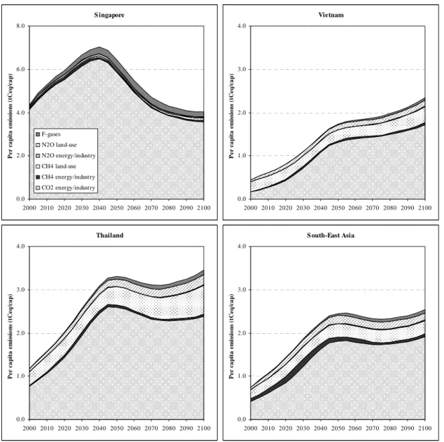
Vietnam 0.0 1.0 2.0 3.0 4.0 2000 2010 2020 2030 2040 2050 2060 2070 2080 2090 2100 P er ca p it a em is si o n s ( tC eq /c a p ) S outh-East Asia 0.0 1.0 2.0 3.0 4.0 2000 2010 2020 2030 2040 2050 2060 2070 2080 2090 2100 P er ca p it a em is si o n s ( tC eq /c a p ) S ingapore 0.0 2.0 4.0 6.0 8.0 2000 2010 2020 2030 2040 2050 2060 2070 2080 2090 2100 P er ca p it a em is si o n s ( tC eq /c a p ) F-gases N2O land-use N2O energy/industry CH4 land-use CH4 energy/industry CO2 energy/industry Thailand 0.0 1.0 2.0 3.0 4.0 2000 2010 2020 2030 2040 2050 2060 2070 2080 2090 2100 P er ca p it a em is si o n s ( tC eq /c a p )

Figure 6.2 Per capita emissions per source for three countries in South-East Asia and the region itself

Figure 6.2 shows the trends in per capita emissions over time in each of the three countries and the region as a whole – broken down by the different greenhouse gases and sources. The per capita emissions converge partly, but not totally, to the regional average. The figure also shows that the composition of different greenhouse gasses across the countries is somewhat different, with fossil fuel CO2 emissions completely dominating emissions from Singapore,

while non-CO2 emissions from agricultural sources constitute an important source in

Thailand. The trends over time show increasing emissions in Thailand and Vietnam

(consistent with their state of development) while emissions in Singapore peak in the middle of the century and decrease as energy intensity improvement outpaces income increases.

(38)

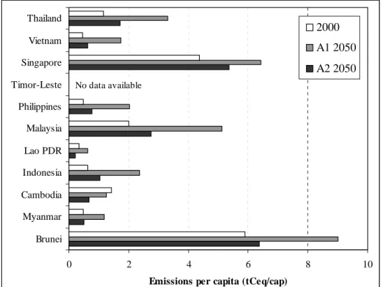
0 2 4 6 8 10 Brunei Myanmar Cambodia Indonesia Lao PDR Malaysia Philippines Timor-Leste Singapore Vietnam Thailand

Emissions per capita (tCeq/cap)

2000 A1 2050 A2 2050 No data available

Figure 6.3 Per capita emission levels for the countries of South-East Asia in 2000 (the base year) and 2050 for the A1 and A2 scenarios

In Figure 6.3 and Table 6.1, we again focus on the results of all countries making up South-East Asia. Figure 6.3 shows that the differences between the scenarios at the regional level are reflected in the downscaling results of the different countries. Table 6.1 compares the method used in this paper (A1b scenario) to the trend methodology applied by Höhne and Ullrich (2005) (Den Elzen (2005) presents a more detailed comparison of the two

methodologies). In this method, the regional trend in total GHG emissions is projected onto national total GHG emissions. This methodology results in large per capita emission levels for countries starting with relatively large per capita emissions (Singapore and Brunei), while countries starting with relatively low per capita emission levels (Timor-Leste, Cambodia, Laos and Vietnam) remain relatively low. The resulting emissions levels for Singapore and Brunei are several times the current OECD average and do therefore not represent a

reasonable outcome. The results of the methodology presented in this paper show that countries with a relatively large per capita emission level have lower growth rates than countries with a relatively low per capita emission level.

(39)

Table 6.1 Per capita emissions for the A1b scenario in 2050 determined using the method published earlier (Höhne and Ullrich, 2005) and the methodology proposed in this study

2000 2050 Annual growth Earlier method This study Earlier method This study

tCeq/cap tCeq/cap tCeq/cap %/yr %/yr South-East Asia 0.7 2.4 2.4 2.4% 2.4% Brunei 5.9 13.7 9.0 1.7% 0.9% Myanmar 0.5 1.7 1.2 2.5% 1.8% Cambodia 1.4 3.0 1.3 1.5% -0.2% Indonesia 0.6 2.2 2.4 2.5% 2.7% Lao PDR 0.3 0.7 0.6 1.5% 1.2% Malaysia 2.0 5.5 5.1 2.0% 1.9% Philippines 0.5 1.3 2.0 2.1% 2.9% Timor-Leste No data available

Singapore 4.4 16.6 6.4 2.7% 0.8%

Vietnam 0.4 1.4 1.7 2.3% 2.7%

Thailand 1.2 4.5 3.3 2.7% 2.1%

Finally, Figure 6.4 presents the downscaled per capita emissions in 2050 for all countries and the yearly increase in the emissions per capita between 2000 and 2050 for both the A1 and A2 scenarios. The emissions per capita are much larger in 2050 in the A1 scenario than in the A2 scenario, despite the higher rate of intensity improvement in A1. For the A1 scenario, the countries with the largest per capita emission increase are the relatively low per capita emission countries in the Southern African and South Asian regions. The same holds for the A2 scenario, although the increases are much lower.

(40)

Figure 6.4 Per capita emission levels in 2050 for the A1 scenario (upper left) and the A2 scenario (upper right), and the annual per capita emissions growth between 2000 and 2050 for the A1 scenario (bottom left) and the A2 scenario (bottom right)

(41)

7 Discussion and conclusions

There are several different types of analyses that require scenario information at a finer scale than that provided by global environmental integrated assessment models. Examples of such analyses include impact and adaptation analyses or climate policy analyses. Several methods have been proposed in the past for downscaling the socio-economic and environmental parameters associated with these scenarios. However, reviews of the results of these simple downscaling methods reproached them for yielding unsatisfactory results.

Different categories of simple, generic algorithms can be used for downscaling: e.g. linear downscaling, convergence and external-input-based downscaling. In this paper, we propose a method for downscaling population data, per capita income levels and emission levels by using a combination of these algorithms. By applying the proposed methodologies to the IPCC-SRES scenarios, we show that they can actually be used to provide information about these scenarios at the level of countries and at the grid level. By comparing the results to those generated by earlier work, we show that the proposed methodologies yield a consistent dataset that does not suffer from the unsatisfactory results of earlier work.

The numerical results, i.e. the datasets created for the four IPCC-SRES scenarios, are

available from the authors. It should be noted, however, that the methodology is not restricted to the IPCC-SRES scenarios alone and other scenarios can also be downscaled using the methodology discussed.

It should also be noted that downscaling methods based on simple algorithms obviously have their strengths and weaknesses. The strengths include the transparency and the relative ease at which regional level data can be made available at a finer scale, without needing to conduct or repeat analysis at this particular scale. The weaknesses certainly include the limitations associated with rule-based downscaling and the methodologies proposed here. The

methodologies are applied independently of population and per capita income levels. In reality though, all kinds of structural relationships exist between these two socio-economic indicators: for example, income is related to mortality and fertility levels but also to the size and quality of the labour force. In addition, various circumstances that are not taken into account (infrastructure; level of education, urbanisation, etc.) may affect the results on the finer scale.

One option for overcoming weaknesses consists of refining the downscaling methodologies further. However, this may come at a cost: while improving quality, making the algorithms

(42)

too detailed detracts from transparency. In some cases, therefore, explicit national-scale modelling might sometimes be more fruitful. Changes that in our view can be made easily, while keeping the downscaling relatively simple, would include 1) exploring alternative convergence algorithms that also account for changes in relative differences over time, 2) separate accounting for large groups within the data such as sectors (industry, services, agriculture), and societal groups (urban and rural), 3) using better data as a basis for downscaling (e.g. sub-national or grid GDP data), 4) developing specific algorithms for distinct emission sources (land-use CO2 emissions).

For many applications, however, we believe that the results of the downscaling approach described in this paper would certainly be sufficient. In our view, downscaling is a way of obtaining credible national and sub-national data, but without creating a perfect dataset for all purposes.