Evaluation of Mixing Height representations in the EUROS model | RIVM

Hele tekst

(1)research for man and environment. RIJKSINSTITUUT VOOR VOLKSGEZONDHEID EN MILIEU NATIONAL INSTITUTE OF PUBLIC HEALTH AND THE ENVIRONMENT. RIVM report 711002 001 Evaluation of Mixing Height representations in the EUROS model L. Delobbe1, J. Matthijsen, F.J. Sauter May 2001. 1. VITO/TAP, Flemish institute for technological research/department for teledetection and atmospheric processes, Mol, Belgium. This investigation has been performed within the framework of the RIVM project S/711002/01/LU (compartimental models), and in cooperation with the Flemish institute for technological research (VITO) through the BelEUROS project (AS/DD/10) financed by the Belgium federal office for scientific, technical and cultural affairs (OSTC).. RIVM, P.O. Box 1, 3720 BA Bilthoven, telephone: 31 - 30 - 274 91 11; telefax: 31 - 30 - 274 29 71.

(2) page 2 of 47. RIVM report 711002 001.

(3) RIVM report 711002 001. page 3 of 47. Abstract The EUROS model is an air-quality model used at the Air Research Laboratory of RIVM for short (day) to long-term (year) for simulations of the (chemical) dispersion of gaseous and/or airborne particulate matter on European scale. This report describes a part of ongoing development and validation work on the model to improve the models generic applicability, which is one of the objectives of the RIVM project compartimental models (now: integration of regional models S711002). It focuses on the representation of dispersion processes, with the goal to improve and evaluate these processes. As such it forms a first step in the revision towards a complete three-dimensional description of the transport module in the EUROS model. The work is performed within the framework of a collaboration between the Flemish institute for technological research (VITO) and RIVM. In EUROS the representation of the mixing layer and horizontal advection is improved. The new EUROS version is extensively tested and mixing layer height values are evaluated with lidar measurements. Model results for ozone concentrations and accumulated exposure (AOT) are evaluated in terms of the different mixing layer representations. The revised calculation of the mixing layer gives a much better representation of the land-sea contrast, with lower mixing heights over sea than over land, during the daytime. An important outcome is that the mixing layer concept, used in EUROS, hinders the validation of modelled concentration levels. Because, in spite of the applied scientific model improvements, modelled AOT40 levels for ozone do not show significant improvement in respect to observations. The main concern in this context is the value of the reservoir layer height in the model, which is interlaced with the mixing layer concept. Therefore, it is anticipated that a more realistic representation of the vertical exchange processes, by describing explicitly three-dimensional advection and diffusion, will improve the EUROS model results significantly, both quantitatively and qualitatively..

(4) page 4 of 47. RIVM report 711002 001. Contents SAMENVATTING................................................................................................................................................5 SUMMARY ...........................................................................................................................................................6 1. INTRODUCTION .......................................................................................................................................7. 2. PARAMETERISATION OF THE MIXING HEIGHT IN EUROS.......................................................9 2.1 DESCRIPTION .............................................................................................................................................9 2.2 SPATIAL MH VARIABILITY ......................................................................................................................10 2.3 COMPARISON WITH LIDAR OBSERVATIONS............................................................................................15 2.4 RECOMMENDATION FOR FUTURE DEVELOPMENT.....................................................................................17 2.4.1 Choice of parameters ....................................................................................................................17 2.4.2 Formulations of the mixing height ................................................................................................18. 3. HORIZONTAL TRANSPORT ................................................................................................................19. 4. SIMULATIONS WITH A VARIABLE MIXING HEIGHT.................................................................21 4.1 LAND PROCEDURE USED OVER WHOLE DOMAIN.......................................................................................21 4.2 DISTINCTION LAND-SEA ..........................................................................................................................24 4.3 IMPACT OF THE VERTICAL DISCRETISATION USED FOR THE HORIZONTAL ADVECTION .............................26 4.4 COMPARISON WITH MEASUREMENTS .......................................................................................................30 4.4.1 Ozone concentrations....................................................................................................................30 4.4.2 Ozone AOT40 ................................................................................................................................33. 5. CONCLUSIONS........................................................................................................................................35. REFERENCES....................................................................................................................................................36 APPENDIX 1 EUROS MODEL RUN DESCRIPTIONS ..........................................................................................38 EFFECT OF MISSING DEFAULT VALUE FOR SENSIBLE HEAT FLUX ...........................................39 APPENDIX 1.1 RUNS TO TEST THE IMPACT OF (NON)UNIFORM MH AND HEIGHT OF RESERVOIR-LAYER TOP40 APPENDIX 1.2 APPENDIX 1.3 RUNS TO TEST THE IMPACT OF THE LAND-SEA DISTINCTION USED TO CALCULATE THE MH .41 RUNS TO TEST THE IMPACT OF THE VERTICAL RESOLUTION USED FOR THE ADVECTION........42 APPENDIX 1.4 VARIOUS OPTIONS FOR THE REPRESENTATION OF THE ADVECTION.......................................43 APPENDIX 1.5 EFFECT OF MH REPRESENTATION ON AOT40: MODEL VERSUS MEASUREMENTS. ................46 APPENDIX 1.6 APPENDIX 2 MAILING LIST ............................................................................................................................47.

(5) RIVM report 711002 001. page 5 of 47. Samenvatting Dit rapport geeft een beschrijving en evaluatie van recente ontwikkelingen die samenhangen met de menglaagbeschrijving in een chemisch transport model voor Europa, het EUROS model. De menglaaghoogte kan in de herziene versie voor elke gridcel worden berekend op basis van meteorologische variabelen in deze grid-cel. De implementatie van deze ruimtelijk variabele menglaaghoogte leidde tot een herziening van de beschrijving van het horizontale transport. Zo is een nieuwe verticale structuur geïmplementeerd om horizontale advectie voor de herziene menglaagversie te kunnen berekenen. De laatste ontwikkeling levert het EUROS model een 3D gridstructuur. De nieuwe versie van het model is uitvoerig getest. De herziene menglaaghoogte beschrijving geeft een veel betere representatie van het land-zee verschil, met lagere menghoogtes boven zee dan boven land gedurende de dag. De menglaaghoogtes die worden afgeleid op basis van de herziene berekeningen zijn vergeleken met observaties van de menglaaghoogte op basis van LIDAR metingen verricht door RIVM/LLO. De gevoeligheid van ozon concentratieontwikkeling in EUROS voor de wijze waarop de menglaaghoogte wordt weergeven bleek erg klein. Deze geringe gevoeligheid is gerelateerd aan de relatief gebrekkige beschrijving van het verticale transport tussen de modellagen. Met name het massatransport tussen de toplaag en de laag daaronder speelt hierbij een belangrijke rol. Deze verticale massatransporten worden impliciet geregeld door de hoogte van de reservoirlaag, een (nachtelijke) laag boven de grenslaag die in het EUROS model een voorgeschreven hoogte moet hebben. De invloed van de verticale discretisatie die wordt toegepast bij de herziene berekening van horizontale advectie is getest. Op basis van deze gevoeligheidsstudie is een verticale structuur van 15 model lagen optimaal met een relatief hoge resolutie tot ongeveer 1500 m. Voor geaccumuleerde blootstellingniveaus van ozon (in dit geval AOT40) bleek dat de doorgevoerde, wetenschappelijk verantwoorde, verbeteringen aan het EUROS model nog geen significante verbeteringen opleverden in de vergelijking tussen model- en meetwaarden van AOT40. De beperkende factor, de voorgeschreven reservoirlaaghoogte, is zo de belangrijkste aanpassingsparameter geworden. Dit ondermijnt een degelijke validatie van EUROS modelresultaten. De verwachtingen zijn daarom dat een minder geparametriseerde beschrijving van het verticale transport zal leiden tot een belangrijke verbetering van de EUROS modelresultaten, zowel kwantitatief als kwalitatief. De hier beschreven nieuwe versie van het EUROS model met een ruimtelijke variabele menglaag en een 3D gridstructuur vormt een eerste stap in de richting van een volledige driedimensionale beschrijving van advectie en diffusie..

(6) page 6 of 47. RIVM report 711002 001. Summary This report describes recent developments of a chemical dispersion model for Europe, the EUROS model. The representation in the model of the mixing layer has been improved: the mixing layer height is calculated for each grid cell from surface meteorological variables. The implementation of this spatially variable mixing layer required a revision of the representation of the horizontal transport. A new multi-layer vertical structure has been implemented for the calculation of the horizontal advection. As a consequence the model is now provided with a quasi three-dimensional structure. The new version of the model has been extensively tested. The revised calculation of the mixing layer allows a much better representation of the land-sea contrast, with lower mixing heights over sea than over land during daytime. The mixing layer heights resulting from the revised parameterisation have been compared with observations, which are based on LIDAR measurements performed at RIVM/LLO. The sensitivity to the representation of the mixing layer of the ozone time evolution in the EUROS model was found to be very low. This low sensitivity is related to the poor representation of vertical exchanges between the model layers. In particular, the mass exchanges with the top layer play here a dominant role. Vertical mass exchanges are implicitly controlled by the height of the reservoir layer top, which is prescribed in the EUROS model. The impact of the vertical discretisation chosen for the calculation of the horizontal advection has also been tested. It is recommended to use a vertical structure with around 15 model layers with a relatively fine resolution up to 1500 m. In terms of AOT40 levels for ozone it was found that the scientific improvements which have been tested do not yet contribute to an improvement of model results when fitted to observations. The main issue in this context is the value of the reservoir layer top in the model. Because in its present description the height of the reservoir layer is arbitrary, the height has become a major adjustment parameter undermining a sound validation of modelled ozone and other tracers. Therefore it is anticipated that a more realistic representation of the vertical exchange processes will improve the EUROS model results significantly, both quantitatively and qualitatively. The new version of EUROS with a spatially variable mixing layer and a three-dimensional grid structure constitutes a first step towards a fully three-dimensional representation of the advection and diffusion process..

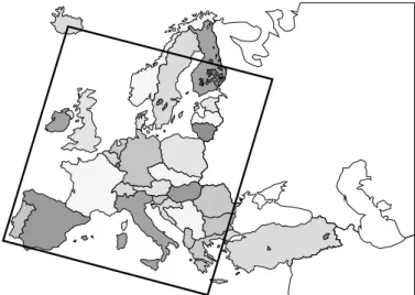
(7) RIVM report 711002 001. page 7 of 47. 1 Introduction The EUROS (EURopean Operational Smog) model is a Eulerian air quality model that has been developed at RIVM. EUROS is and will be used to evaluate possible policy measures for LRTAP issues (Long Range Transboundary Air Pollution) in for instance environmental assessments and outlooks. In order to comply with the present state of science, air quality models require development and revision of the modelled processes. This report describes recent developments and a revision of the vertical structure in connection with transport processes in the EUROS model. The EUROS model has originally been developed to model winter-smog episodes (SO2) in Europe (van Egmond and Kesseboom, 1981). Later, the model has been used to study the temporal and spatial behaviour of not only SOx and NOx, but also of groundlevel ozone (O3), volatile organic compounds (VOC’s) and persistent organic pollutants (POPs) in the lower troposphere over Europe. At present EUROS is being extended to model the dispersion of particulate matter (PM10). The present EUROS version models emissions, transport processes, chemical transformation, dry and wet removal processes and first order degradation in soil and water of various compounds. This and earlier versions of the EUROS model are described in Jacobs and Van Pul (1996), Van Loon (1996), Rheineck Leyssius and De Leeuw (1990, 1991), De Leeuw and Rheineck Leyssius (1990), De Leeuw (1987), De Leeuw et al. (1985, 1986), Van Egmond and Kesseboom (1981).. Figure 1.1 The EUROS model domain (encapsulated by the box) The modelled area extends over a large part of Europe (figure 1.1). The horizontal base grid consists of 52 x 55 grid cells with a 0.55° x 0.55° longitude-latitude resolution on shifted pole co-ordinates (about 60 x 60 km2). Local uniform grid refinement is possible up to 4 levels resulting in a maximum longitude-latitude resolution of about 0.069° x 0.069° (about 7.5 x 7.5 km2). Grid refinement is possible in a dynamic way, where a higher resolution is taken if the concentration gradient between adjacent grid-cells exceeds a certain threshold value. Grid.

(8) page 8 of 47. RIVM report 711002 001. refinement is also possible for areas of special interest, for instance The Netherlands. In the original version of EUROS (van Loon, 1996), the vertical structure consists of four layers: the surface layer (SL), the mixing layer (ML), the reservoir-layer (RL) and the toplayer (TL). The depths of the four layers are uniform over the whole domain but vary in time during the day due to the growth of the mixing layer, except for the surface layer whose depth is fixed at 50 m. The mixing layer growth during day hours is represented through a constant climatological growth rate. The climatological representation of the mixing height (MH) has been recently revised in order to take into account the effect of meteorological conditions on the ML growth. This resulted in a version where the MH is calculated from surface meteorological variables using simple parameterisations found in the literature. In a first step, this method has been applied for a single grid cell located in the Netherlands and the derived MH used for the whole of Europe. This approach allowed to maintain a two-dimensional structure with uniform model layer depths. This study is devoted to the next step, consisting in applying this method for each grid cell of the domain. This causes the mixing layer to become spatially non-uniform. The implementation of a spatially variable mixing layer requires a new representation of the horizontal advection. A new vertical structure including a number of thin uniform layers has been implemented for the calculation of horizontal advection. The number of layers can be easily modified. This provides the model with a three-dimensional grid structure. However, the representation of the advection remains two-dimensional. It does not take into account the vertical advection. This report is organised as follows. In the next section, the implementation of a spatially variable mixing height is described. The comparison of simulated mixing heights with LIDAR observations is also presented. The adaptation of the horizontal advection scheme is described in section 3. The new version of EUROS has been extensively tested. The results are analysed and compared with the observations in section 4. Finally, general conclusions are drawn in section 5..

(9) RIVM report 711002 001. page 9 of 47. 2 Parameterisation of the mixing height in EUROS 2.1 Description The description of the EUROS model in Van Loon (1996) serves in this report as reference. De Leeuw and Van Rheineck Leyssius (1990) describe the diurnal evolution of the mixing layer with a simple parameterisation (see also Van Loon, 1996). The MH is defined as being constant during the night (300 m) and grows with a constant rate during day time. After sunset, the nocturnal mixing layer is re-established. The growth rate of the ML during the day is prescribed according to climatological values for mid latitudes. Growth rates are 50 and 75 meters per hour, for winter and summer, respectively. The MH varies in time but is the same for the whole of Europe at one specific moment. The above representation of the ML has been updated with a new method for the calculation of the MH. The present calculation is based on diagnostic formulas which relate the MH to surface meteorological variables. These parameters are the friction velocity (u*), the Obukhov length (L), and the sensible heat flux (hs). Three different cases are considered for the calculation of the MH (H): Stable atmospheric conditions (L > 0 m): The atmospheric boundary layer is considered as stable if the Obukhov length is positive. In this case, the MH is calculated following Nieuwstadt (1981a and 1981b): c1u * / fL H = L 1 + c2 H / L. (2.1). with the constants c1 = 0.15 and c2 = 0.31, and Coriolis parameter, f, is 0.0001 s-1. This formulation is also discussed in Holtslag and Westrhenen (1989). It must be solved iteratively. The initial value is given by the MH value under neutral conditions. Neutral conditions (L < -1000 m): For strongly negative Obukhov lengths, the boundary layer is considered as neutral. The following expression is then used : H = c1u * / f. (2.2). Note that (2.2) is the limit of (2.1) for increasing values (negative or positive) of the Obukhov length (L). Unstable conditions (-1000 < L < 0 m): In unstable cases, the growth of the convective mixing layer is described with a prognostic equation. The formulation of Tennekes (1973) is used: h ∂H = s (2.3) ∂t γ H where γ is the vertical gradient of potential temperature above the convective boundary layer..

(10) page 10 of 47. RIVM report 711002 001. This model considers the surface heating flux as the only relevant driving force, neglecting other contributions like the mechanical turbulence production due to surface friction. The parameter γ expresses the stability of the layer above the convective layer. Its value is fixed to the climatological value of 0.005 K/m. The integration of (2.3) over one time step results in:. H t +1 =. H t2 +. 2∆t hs ,t. γ. (2.4). The surface meteorological parameters u*, L, and hs are calculated using a software library developed at KNMI (Beljaars and Holtslag, 1990). Input parameters are wind velocity (at 10 m for example), surface air temperature (at 2 m), aerodynamic roughness length and cloud cover from synoptical observations. Input data are taken from the gridded NCAR synop observations (referred to as ODS, observational data set; Potma, 1993). For CPU efficiency reasons and in order to avoid application difficulties with horizontal advection, a uniform mixing layer over Europe is used. The calculation of the mixing layer height is carried out for a single grid cell located in The Netherlands and this value is applied to the whole of Europe. Clearly, this method leads to rather coarse representation of the MH, which varies in reality not only in time but also in space. The following step, therefore, consists in calculating the MH for each grid cell of the EUROS domain. This improvement includes a thorough revision of the advection scheme so that it works in case of a spatially variable mixing layer. The adaptation of the advection scheme is described in section 3. The KNMI software for the calculation of the surface parameters was developed for use over horizontally homogeneous flat terrain and validated with observations at Cabauw in The Netherlands. Over complex terrains, these routines are not expected to yield accurate results. This must be kept in mind when using these routines over all European regions. Besides, some internal parameters used in these routines (the ground albedo for example) are not adapted to regions other than The Netherlands. This point will be discussed in section 2.2.3. Finally, the KNMI routines which have been implemented in EUROS are designed for the calculation of the ML over land and not over sea. The calculation of the MH over sea needs the implementation of new routines suited to those conditions.. 2.2 Spatial MH variability An important improvement of the ML representation in EUROS consists in calculating the MH for each EUROS grid cell and not for one grid cell located in The Netherlands. Large areas of the EUROS domain are sea areas and it is therefore necessary to extend the determination of the MH to sea conditions. The expressions used in EUROS (2.1, 2.2, 2.3) for the calculation of the MH, as well as those reviewed in Seibert et al. (2000) are based on three meteorological variables i.e., the Obukhov length, the friction velocity and the sensible heat flux. To evaluate these parameters over sea, the adequate routine from the KNMI software library is implemented in EUROS, i.e. the routine FLXSE1 from Beljaars and Holtslag (1990)..

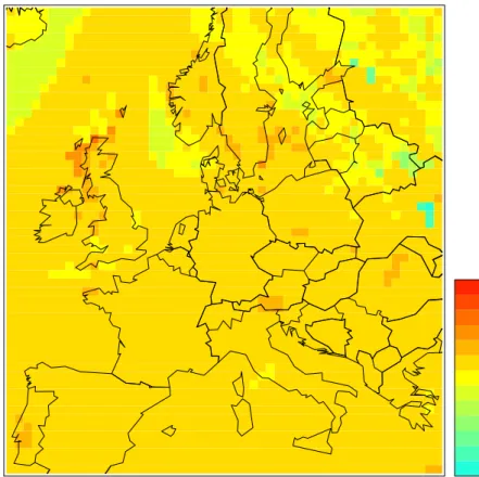
(11) RIVM report 711002 001. page 11 of 47. The input meteorological data for the routine FLXSE1 are the sea surface temperature (SST), the air temperature and a single wind speed. The two latter variables are provided for by ODS. For the SST, monthly climatological values are used as a first approximation. This approximation is quite valid since the SST evolution along the year is relatively slow and remains similar from one year to the other. The monthly SST climatology from Trenberth and Reynolds from NCAR (Boulder, USA) is used (Shea et al., 1990; Shea et al., 1992). It provides monthly averaged SST values with a regular 2 degrees spatial resolution. The calculation of the three variables u*, L, hs using FLXSE1 does not converge if the wind velocity is too small. In unstable conditions (SST larger than the surface air temperature), the wind velocity must be at least 1.5 m/s to ensure convergence. In stable conditions (SST smaller than surface air temperature), the wind must be at least 3.8 m/s. To avoid convergence failure in the calculation of the meteo parameters, minimal values of the wind velocity have been set to 2 and 4 m/s for unstable and stable conditions, respectively. Note also that a zero default value for the sensible heat flux has been prescribed (Appendix 1.1). Figures 2.1 and 2.2 illustrate the impact of the land-sea distinction on the geographical pattern of the mixing layer height (runs 641 and 642, conform Appendix 1.3). The mixing layer depth calculated by EUROS is shown for 30 July 1990 at 04 UT (figures 2.1 and 2.2) and at 16 UT (figures 2.3 and 2.4). Note that the top of the mixing layer is given by the ML depth plus 50m, which is the depth of the surface layer. When the land-sea distinction is not included, the calculated mixing layer heights are similar over land and over sea, as well during the night as during the day. This is not realistic. In contrast with land, the sea surface temperature is almost constant at the day scale. No diurnal cycle is observed. This results in a stabilising effect during the day (SST is cooler than the atmospheric temperature) and a destabilising effect during the night. Over land, the opposite effect is observed with strong destabilising effect during the day, due to surface heating and a strong stabilisation during the night due to the longwave cooling of the land surface. When the “land routines” are used everywhere, this effect can not be accounted for. As shown in figures 2.2 and 2.4, the geographical pattern of the calculated MH is significantly improved. During the night, higher MHs are obtained over sea while during the day, stabilisation over sea results in relatively low ML values in comparison with those obtained over land. A common feature of figure 2.2 and 2.4 is that the western border of some land areas exhibit a systematic higher MH than the sea and land grid points around. This is particularly true for the north of UK and Ireland, and the south of Portugal. This shortcoming is probably related to the interpolation of surface meteo data for grid cells that are partly over land and partly over sea. Note that for sea grid cells, this deficiency disappears when the land-sea distinction is introduced (see north of UK)..

(12) page 12 of 47. RIVM report 711002 001. Finally, let us remark that the geographical pattern of the MH clearly shows that significant areas of The Netherlands located near the coast are modelled as sea areas. This must be kept in mind when the simulated results are compared with measurements collected in stations near the coast..

(13) RIVM report 711002 001. page 13 of 47. dzlay. m 2400 2000 1500 1250 1000 750 500 250 200 150 100 50 0. Figure 2.1: Mixing layer depth at 04 UT for July 30, 1990. Spatially variable mixing height. No land-sea distinction in the calculation procedure. dzlay. m 2400 2000 1500 1000 750 500 250 200 150 100 50 0. Figure 2.2: Mixing layer depth at 04 UT for July 30, 1990. Spatially variable mixing height with land-sea distinction.

(14) page 14 of 47. RIVM report 711002 001. dzlay. m 2400 2000 1500 1250 1000 750 500 250 200 150 100 50 0. Figure 2.3: Mixing layer depth at 16 UT for July 30, 1990. Spatially variable mixing height. but no land-sea distinction in the calculation procedure dzlay. m 2400 2000 1500 1000 750 500 250 200 150 100 50 0. Figure 2.4: Mixing layer depth at 16 UT for July 30, 1990. Spatially variable mixing height with land-sea distinction.

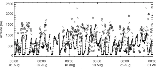
(15) RIVM report 711002 001. page 15 of 47. 2.3 Comparison with LIDAR observations The validation of the parameterisations used for the calculation of the mixing layer height is of crucial importance but remains a problematic issue. Observations of the atmospheric boundary layer are only available for some specific locations, most of them over land, which makes a validation on European scale difficult. We have compared the MH calculated by EUROS for the grid cell which includes Bilthoven with the RIVM LIDAR observations. The LIDAR determination of the MH is based on the backscatter of a laser beam by aerosol particles present in boundary layer (van Pul et al., 1994). The top of the MH is marked by a discontinuity in the backscatter profile. The comparison has been performed for August 1994. Figure 2.5 shows two time evolutions of the MH. Significant discrepancies between the two time series are found. The LIDAR observations exhibit a much larger variability than the EUROS values. For most days, the MH estimated by EUROS is 100 m during the night and grows in a monotonic way up to a value around 1000 m in the late afternoon. According to the LIDAR observations the night values of the MH are mostly between 200 m and 700 m. During day time, the MH is usually comprised between 1000 and 1500 m but sometimes exceeds 2000 m. LIDAR observations exhibit significant variations during day time in contrast with the day time values obtained with the EUROS parameterisation.. Figure 2.5 Comparison of the mixing layer height estimated by the EUROS model (solid line with diamonds) and derived from LIDAR observations at RIVM (open circles) for August 1994. Figure 2.6 shows the averaged diurnal cycle for August 1994 as observed with the LIDAR and simulated by EUROS. It appears that EUROS tends to underestimate the MH. During the day the mean difference between the LIDAR and EUROS values for August 1994 is limited to about 200 m. In the night the differences in the mean MH are considerably larger. It must be noted that the lowest ML top that can be detected by the LIDAR is about 200 m. If the actual ML top is lower than 200 m, the LIDAR may consider the top of a residual layer as the.

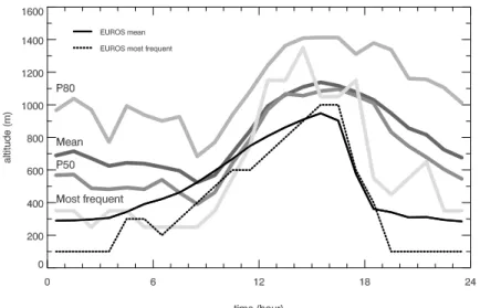
(16) page 16 of 47. RIVM report 711002 001. ML top leading to an unrealistically high MH. The night time mean MH values are strongly affected by these erroneous MH estimates. In the evening, it may also take some time until the LIDAR may detect the top of the new boundary layer, within the previously well-mixed layer. Figure 2.7 shows the boundary layer climatology for August at Bilthoven, based on the lidar observations for 1992 to 1999. During the night, the mean value strongly differs from the most frequent value, which is around 300 m. For the EUROS results, the differences between the mean values, the most frequent values and the 50-percentile are much more limited. The comparison between the average diurnal cycle for August 1994 and the averaged LIDAR diurnal cycle (figure 2.6) shows a relatively good agreement.. Figure 2.6 Average mean values and most frequent values of the mixing layer height at Bilthoven for August 1994, as estimated by the EUROS model and derived from the LIDAR measurements at RIVM. Figure 2.7 Mixing height diurnal cycle (P80=80 percentile, Mean, P50=50 percentile and Most frequent). Climatology for August derived from LIDAR measurements at Bilthoven (RIVM) of the years 1992 – 1999 (thick gray lines) and EUROS model estimates of the average mean (thin solid line) and most frequent MH values (thin dotted line) at Bilthoven for August 1994 (as in figure 2.6)..

(17) RIVM report 711002 001. page 17 of 47. As far as the time series for the month August are concerned (figure 2.5), several causes of discrepancies can be mentioned. First of all, the method used in EUROS for the calculation of the MH has its own limitations. Errors may arise from the calculation of the surface meteorological parameters (Obukhov length, friction velocity and heat flux) through the KNMI routines but also from the determination of the MH from these parameters using expressions (2.1), (2.2) or (2.4). The meteo input used for the calculation of the surface meteo variables, for example the 2-m-temperature and the 10-m wind, also induce some errors. The meteo input used in EUROS results from a spatial interpolation from synoptic observations and a time interpolation from the 4 input times of these synoptic observations (00, 06, 12, 18 UT). This interpolation partly explains the fact that the ML diurnal cycles simulated by EUROS are much smoother than the observed diurnal cycles from the LIDAR. Another possible cause of discrepancies arises from the fact that the LIDAR observations are local while the EUROS estimate is an average over a 60 x 60 km2 grid cell. Finally, the determination of the MH from LIDAR measurements has also its own limitations. We have already mentioned the minimal detectable value of 200 m which may result in large errors for the night estimates. Another shortcoming is the large inaccuracies in case of rain or if the amount of aerosol or trace gas in the boundary layer is too low. This discussion explains that a much larger variability is obtained in the LIDAR data than in the MH simulated by EUROS. A more extensive validation of the MH parameterisation in EUROS would involve a comparison with various observational data, including observations from LIDAR and soundings, but also with results of atmospheric models with detailed representation of the boundary layer processes (Delobbe et al., paper in preparation).. 2.4 Recommendation for future development Further development of the mixing layer concept consists of a spatial differentiation of surface parameters and application of an extended parameterisation of the MH which includes a description for mechanical and entrainment processes which contribute significantly to the growth of the MH. The comparison with LIDAR measurements (section 2.3) forms the incentive for the latter development.. 2.4.1 Choice of parameters The parameterisations used to calculate the surface parameters (u*, L, and hs) contain a number of empirical coefficients which have been optimised for data gathered at Cabauw in The Netherlands. The values of these coefficients are typical for grassland with sufficient water supply on a clay soil. Beljaars and Holtslag (1990) mention that the most important parameters are the albedo, the modified Priestley-Taylor parameter (which controls the partitioning of available surface energy between latent and sensible heat flux), and the bulk soil heat transfer coefficient (which relates the heat flux into the soil to the temperature.

(18) page 18 of 47. RIVM report 711002 001. difference between the top of the vegetation layer and the deep soil). When the KNMI software library is used for different terrain types, it is recommended to adapt these parameters. Beljaars and Holtslag (1990) suggest some guidelines to determine the parameters from local land-use conditions. The relationships they propose are mainly based on Stull (1988). In the new version of the EUROS model, allowing a variable mixing layer height over Europe, it could be useful to adjust the above-mentioned parameters for each grid cell as a function of the land-use conditions. Note that the mesh of the base grid of Euros may contain various land-use types and an adequate interpolation procedure should be applied. Another parameter which influences the calculation of the MH is the vertical gradient of potential temperature above the convective boundary layer (γ in equation 2.3). This parameter controls the growth of the convective boundary layer in unstable conditions. Its value is fixed to 0.005 K/m in EUROS. Observations show a large variability of γ (e.g., van Pul et al., 1994). A better determination of this parameter may be investigated.. 2.4.2 Formulations of the mixing height The expressions (2.1), (2.2) and (2.4) to calculate the mixing height may be updated according to recent literature. A review of operational methods for the determination of the mixing height is made in Seibert et al. (2000). The calculation of the MH in stable or neutral conditions remains a very controversial issue and a large variety of formulations have been proposed. These formulations differ through the choice of the meteorological input parameters (Obukhov length, Ekman length, friction velocity, Brunt-Väisälä frequency etc.). A wide range of different constants is also used in the same expressions. So far, none of these formulations appears to be fully satisfying and further development and validation work is needed. In case of convective situations, the MH is usually determined through a prognostic equation similar to (2.3) describing the growth of the mixing layer through surface heating. The basic input parameters of these formulations are the surface heat flux and an initial temperature gradient as in the expression (2.3) used in EUROS. These formulations can be improved by taking into account the additional turbulence production due to surface friction as well as the entrainment heat flux at the top of the boundary layer. The entrainment flux is generally parameterised in term of the surface heat flux. For example, the following expression proposed by Batchvarova and Gryning (1991) can be used, 3. h u* ∂H = (1 + 2 A) s + 2 B γH ∂t γ βH 2. (2.5). where hs is the surface heatflux, u* the friction velocity, γ the potential temperature gradient above the MH (H), and β is the buoyancy parameter (β = g/T). The parameters A and B, given in the literature, differ considerably ranging from 0 to 1 for A (A=0 corresponds to no entrainment flux) and between 0 and 10 for B (B=0 corresponds to no mechanical production of turbulence). A discussion on these parameters can be found in Seibert et al. (2000)..

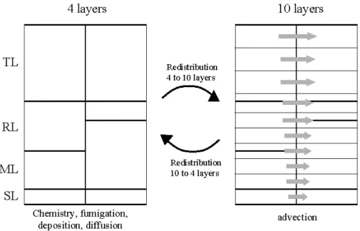
(19) RIVM report 711002 001. page 19 of 47. 3 Horizontal transport The vertical structure of the EUROS model consists of four layers: the surface layer (up to 50 m), the mixing layer, the reservoir-layer, and the top-layer (up to the model top at 3000 m). Advection is taken into account in the mixing layer and the reservoir-layer. Top-layer concentrations determine the upper boundary conditions. These concentrations vary monthly and with latitude. In the case of uniform ML and RL over the whole domain, the computation of the horizontal advection can be easily performed. In the new EUROS version, the implementation of a variable mixing layer height requires a revision of the representation of the horizontal advection process. Several options have been considered and are described in Appendix 1.4. An important criterion in evaluating the various options is the possibility to include vertical advection, allowing EUROS to evolve towards a fully three-dimensional structure. Hereafter we only describe the option that has been selected. A new vertical structure is used for the calculation of the horizontal advection (figure 3.1). It includes layers with fixed boundaries, the number of layers is larger than the initial 4 layers structure. The new multi-layer structure is uniform over the whole domain. It allows to calculate horizontal advection in each advection layer using the same numerical advection scheme as in the initial four-layer structure. In order to keep the computational cost acceptable, a hybrid solution is constructed. The initial four-layer structure is conserved for the calculation of processes other than advection, i.e. chemistry, fumigation, dry and wet deposition, and diffusion.. Figure 3.1 Vertical structure used for advection (right) and for the other processes. Although horizontal advection and fumigation (exchange between the ML and the RL due to change in the mixing layer depth) are coupled processes in reality, they are treated separately in the model. This may lead to mass exchange between the ML and the RL through.

(20) page 20 of 47. RIVM report 711002 001. horizontal advection. This mass exchange may be artificial but it also occurs in more complex 3D atmospheric models. In these 3D models, an advection scheme computes the transport by the mean wind while a turbulence scheme computes the fluxes (mainly vertical) due to turbulence. In EUROS, the mixing layer concept can be considered as a very simple turbulence scheme: a mixing height is determined from meteo data and it is assumed that the atmosphere is well mixed from the ground up to the mixing height. A strong advantage of the hybrid method is that it provides the model with a 3D grid structure which allows implementation of a 3D advection scheme. Besides, it gives the possibility to implement a more sophisticated turbulence scheme. Another improvement is that the vertical profile of the horizontal wind can be better represented in respect to other approaches, in which a four-layer structure is conserved for the advection. Furthermore, it allows a better calculation of the vertical wind when 3D advection is considered. The main disadvantage is the relatively high computing cost. In a first step we consider 10 layers for the calculation of the advection. The impact of the number of layers and the heights of these layers are presented in section 4.3. Another difficulty arises from the fact that the MH does not necessarily correspond with one of the vertical levels of the multi-layer structure. Just before and after the advection step, mass is redistributed from the four meteorological layers to the advection layers, using linear interpolation. This means that numerically induced mass exchange between the vertical layers will occur. Even if the MH remains constant in time, artificial exchange between the ML and the RL will occur through the redistribution procedure between the two vertical structures. Another approach could be to impose that the mixing layer top be equal to one of the advection levels. This approach consists in using an approximate value of the mixing height which is equal to one of the advection levels. It must be kept in mind that the mixing height can not be estimated with great accuracy (e.g. Delobbe et al., 2000). If the error on this estimate is of the same magnitude as the depth of the advection layers, it is justified to approximate the mixing height to the closest vertical level of the multi-layer structure. As a first step, the redistribution procedure is used. The impact of this procedure is presented in section 4.3 dedicated to the sensitivity to the vertical resolution. The standard vertical grid structure includes ten advection layers with boundaries at 50, 100, 200, 400, 600, 900, 1200, 1500, and 2000 m. The horizontal wind used for each advection layer is computed through a linear interpolation from the 5 vertical levels of the meteo input data. Note that the number of layers and the heights of these layers can be easily modified..

(21) RIVM report 711002 001. page 21 of 47. 4 Simulations with a variable mixing height A large number of simulations have been carried out to test the new version of EUROS, which includes a spatially variable mixing height and a multi-layer vertical structure for the representation of the horizontal advection. First, the mixing layer height has been calculated using the “land procedure” over the whole domain. It means that the MH is spatially variable over Europe but the same calculation method is used without distinction over land and over sea. The results are presented in the next section. The simulations including the land sea distinction are described in section 4.2. The sensitivity of ozone time series to vertical discretisation is addressed in section 4.3. The last section (4.4) is devoted to the comparison of the EUROS results with observational data, in terms of concentrations and AOT40. The time period of these simulations concern summer 1990. Hereafter, we summarise the most relevant results and only a limited number of runs are mentioned. An inventory of all simulations can be found in Appendix 1.. 4.1 Land procedure used over whole domain The impact of a spatially variable mixing height is illustrated in figure 4.1. This figure shows the ozone evolution at observation height for runs 618 and 619. In run 618, the MH is uniform over Europe and calculated according to a climatological growth rate during the day. In run 619, the MH varies from one grid cell to another and is calculated from surface meteo parameters following the procedure described in section 2.1. In both simulations, the advection is calculated using a 10-layer vertical structure. The simulation period extends over 6 days from July 30 to August 4 1990. The ozone evolutions have been checked for 14 locations in Europe (mostly in The Netherlands). It appears that the differences between the two simulations for ozone are rather limited and do not tend to grow in time. This is illustrated in figure 4.1. for two specific locations: Cabauw in The Netherlands (between Rotterdam and Utrecht) and Waldhof in Germany (South of Hamburg). The comparison between the two simulations shows that the impact of the ML representation on ozone time series is limited. The MH appears not to be a dominant factor in the evolution of ozone concentrations, as simulated by this version of EUROS. This behaviour seems to be in contradiction with earlier studies (e.g., Vogelezang and Holtslag, 1996). A possible explanation is related to the representation of the vertical exchange between the mixing layer, the reservoir-layer and the top-layer in EUROS. In particular, the altitude of the top of the reservoir-layer, which is prescribed, can play an important role. In the standard version of EUROS, the RL top is fixed to 600 m. In the morning hours, the growth of the mixing layer gives rise to mass exchange between the mixing layer and the reservoir-layer, provided that the ML top does not exceed 600 m. If the MH exceeds 600 m, the reservoir-layer vanishes and an exchange process acts between the mixing layer and the top-layer. Since the concentrations in the top-layer are fixed, the entrainment of mass from the top-layer into the.

(22) page 22 of 47. RIVM report 711002 001. ML constitutes a restoring toward the top-layer background concentrations. The exchange mechanism also implies an intense outflow of mass from the ML to the top-layer at the end of the day when the ML collapses. This outflow flux is implicitly controlled by the prescribed height of the reservoir-layer.. a). b) Figure 4.1 Ground level ozone evolution simulated by EUROS for the measurement stations a) Cabauw and b) Waldhof. Solid line for a spatially variable mixing height (run 618), and the dotted line for a uniform mixing height over Europe (run 619). These considerations let appear that the ozone concentrations in EUROS may be much more affected by the height of the reservoir-layer and the top-layer concentrations rather than by the MH. In order to point out the impact of the reservoir-layer height, a run with a prescribed height of 1500 m has been carried out (run 620). The comparison between run 618 and run 620 is illustrated in figure 4.2. The only difference between the two runs is the prescribed height of the reservoir-layer. Significant differences between the two simulated ozone evolutions are found. A factor of 2 difference in ozone concentrations can be reached in the afternoon hours. The ground level simulated ozone concentrations are higher when the reservoir-layer top is set to 1500 m. This probably results from the reduced mass outflow from the mixed layer to the top-layer at sunset. The MH estimated by EUROS rarely exceeds 1500 m. At the end of the day, when the mixing layer collapses, the mixing layer.

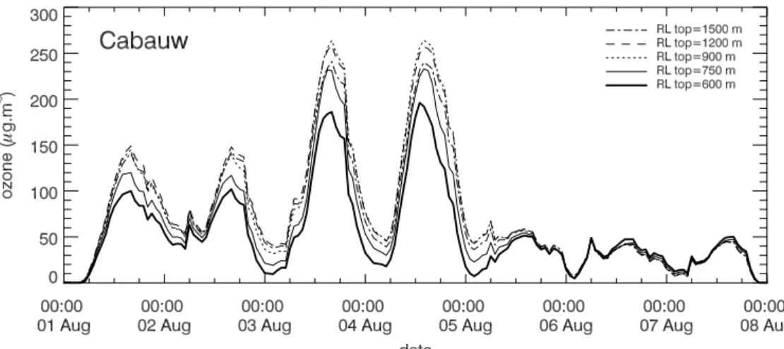
(23) RIVM report 711002 001. page 23 of 47. concentrations are injected in the reservoir-layer and not in the top-layer. The day after, these reservoir concentrations can be entrained again into the mixing layer during the mixing layer growth that occurs in the morning hours.. a). b) Figure 4.2 Impact of the reservoir-layer top on the ground level ozone evolution simulated by EUROS for the measurement stations a) Cabauw and b) Waldhof. Solid line for a reservoirlayer top at 600 m (run 618), and the dotted line for reservoir-layer top at 1500 m (run 620). In order to better catch the impact of the reservoir-layer top, 1-month simulations with various RL tops ranging from 600 to 1500 m have been carried out. The results are illustrated in figure 4.3. For a better visualisation, only the first 8 days of the simulation are plotted. A similar behaviour is found for the following days. The simulated ozone evolution at Cabauw shows again a large sensitivity to the reservoir-layer top. The differences between the various runs are significant. When the RL top is set to 600 m, the exchange with the top-layer is very intense which amplifies the restoring towards the background concentrations of the top-layer. When the RL top is set to 1500 m, the exchange with the top-layer is extremely low. All pollutants present in the surface layer, in the mixing layer and the reservoir-layer remain in these layers. Mass exchanges occur between these three layers but the global mass remains constant. As a consequence, the peak concentrations will be higher. Figure 4.3 shows that peak concentrations are even larger when the RL top is fixed to 900 or 1200 m. The reason of.

(24) page 24 of 47. RIVM report 711002 001. this feature is that the mixing layer top rarely exceeds 1000 m, which means that, even with a RL top around 1000 m, the exchanges with the top-layer will be very limited. With a RL around 1000 m instead of 1500 m, the pollutants are dispersed over a thinner atmospheric layer, which causes the concentrations to increase. In short, the peak concentrations tend to be higher if the RL top is fixed to the maximum value of the MH.. Figure 4.3 Impact of the RL top on the ground level ozone evolution simulated by EUROS for the measurement station Cabauw. The thick solid line for a RL-top at 600 m (run 618), the thin solid line for RL top=750 m (run 627), the dotted line for RL top=900 m (run 624), the dashed line RL top=1200 m (run 625) and the dash-dotted line for RL=1500 m (run 620). In order to limit the computing cost, the above-described simulations have been carried out with the 4-layer vertical structure for the representation of the advection and a uniform mixing layer height. The simulation results with a RL top at 600 m appear to be slightly different from the results obtained with a uniform MH but using a 10-layer structure for the advection. This suggests that the number of layers used for the advection could have a significant impact. This will be further investigated in section 4.3. The conclusion of this section can be summarised as follows. The prescribed value of the reservoir-layer top has a strong impact on the simulation results since it implicitly controls the exchange between the top-layer and the lower layers (reservoir-layer and mixing layer). In other words, it controls the mass exchanges between the boundary layer and the free troposphere.. 4.2 Distinction land-sea As described in section 2.2, new routines have been implemented in order to make a distinction between land and sea for the calculation of the mixing height. The impact on the estimated MH pattern has been described in section 2.2. In this section, we point out the impact on the simulated ozone concentrations..

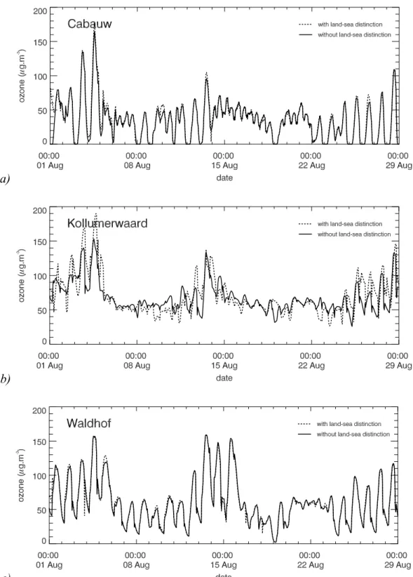
(25) RIVM report 711002 001. page 25 of 47. a). b). c) Figure 4.4 Impact of the land-sea distinction in the calculation of the mixing height. Ground level ozone evolution simulated by EUROS for the measurement stations a) Cabauw, b) Kollumerwaard and c) Waldhof. The results represented by the solid line are without landsea distinction (run 626) and by the dotted line are with land-sea distinction (run 644) in the calculation of the MH. Figure 4.4 illustrates the comparison between run 626 and run 644. These are two 1-month simulations with a spatially variable MH and a 10-layer vertical structure for the horizontal.

(26) page 26 of 47. RIVM report 711002 001. advection. In both simulations, the top of the reservoir-layer is set to 600 m. In run 626, the MH is calculated using for the whole domain the “land routines” while a distinction is made between land and sea grid cells in run 644. This allows a better representation of the land sea contrast in the development of the mixing layer, especially during the day where convective conditions mostly prevail over land while stable conditions and thin mixing layers are found over sea. Over land, the calculated MH is the same in the two simulations. The ozone evolutions are shown for 3 locations: Cabauw, Waldhof, Kollumerwaard. For Cabauw and Waldhof, the ozone evolutions are almost identical. This shows that a change in the MH over sea does not influence the ozone evolution in these two locations. The same conclusion is found for all stations located over land. For stations located at the coast, things can be quite different. Kollumerwaard is located at the northern coast of The Netherlands. As apparent in figure 4.4, significant differences are found between the two simulations. In fact, the grid cell where Kollumerwaard is located is considered by the EUROS model as a sea grid cell. During day hours, the pollutant concentrations remain confined in a relatively shallow mixing layer, which probably explains the higher ozone peaks which are obtained when the land-sea distinction is taken into account. This example shows that model results obtained for coast grid cells must be carefully interpreted. The results of this section can be summarised as follows. The impact of the land-sea distinction for the MH calculation on the ozone time series is in the present EUROS version negligible for land locations. The impact is only significant at the coast or over seas.. 4.3 Impact of the vertical discretisation used for the horizontal advection Up to here, all the simulations have been carried out with a ten-layer structure for the representation of the horizontal advection process. The heights of the ten levels were 50, 100, 200, 400, 600, 900, 1200, 1500, 2000 and 3000 m. The number of levels and the heights of these levels influence the re-distribution of the concentrations from the four-layer structure (SL, ML, RL and TL) to the multi-layer structure used for the advection. Therefore, it is useful to investigate how sensitive the results are to the vertical discretisation used for the advection. The vertical grid structures which have been tested are represented in table 1. The period of simulation is August 1990. In all the simulations, the mixing layer is calculated from the surface meteo parameters with distinct procedures for land and sea. The top of the reservoir-layer is fixed to 600 m. The simulated ozone time series for Cabauw and Waldhof are presented in figure 4.5. It is not apparent in the plots but the simulations 660 and 665 give exactly the same results (the thick solid line is hides the thin triple-dot-dash line). Simulation 663 gives also almost identical results..

(27) RIVM report 711002 001. page 27 of 47. a). b) Figure 4.5 Ground level ozone evolution simulated by EUROS for the measurement stations a) Cabauw and b) Waldhof.The simulations have been done with various vertical discretisations for the calculation of the advection, which are described in table 1 section 4.3. In the first four runs, the advection is calculated using 10 layers. It appears that simulation 662 strongly differs from the three other simulations with ten layers. The only difference between the vertical discretisation in runs 662 and 663 is the height of the fifth level, which is respectively at 700 and 600 m. In run 662, no advection level is located at the top of the reservoir-layer, which is set at 600 m. It means that at each advection step, an artificial exchange between the reservoir-layer and the top-layer occurs through the redistribution procedure. This shortcoming does not occur when the reservoir-layer has vanished due to the growth of the mixing layer. Nevertheless, during the night and the morning hours, the artificial exchange with the top-layer causes a strong restoring toward the top-layer background concentrations, leading to an outflow of precursor concentrations from the boundary layer to the free troposphere. It results in a reduced ozone production during the day. This explains why lower ozone concentrations are obtained when the top of the reservoir-layer does not match one of the advection levels.

(28) page 28 of 47. RIVM report 711002 001. Table 1: Vertical grid structures used in different (test) runs. run nr. 660 661 662 663 # layers 10 10 10 10. 664 15. 665 15. 3000 2900 2800 2700 2600 2500 2400 2300 2200 2100 2000 1900 1800 1700 1600 1500 1400 1300 1200 1100 1000 900 800 700 600 500 400 300 200 100 50. In runs 664 and 665, the advection is calculated using 15 layers. In run 664, a fine resolution is used in the lower layers while in run 665, a more uniform distribution is used from the surface up to 3000 m. Note that in both cases, one of the advection levels is located at 600 m. In run 665, the vertical levels up to 1200 m are exactly the same as in run 660. The results of run 660 and 665 are identical which means that it has no use to refine the resolution in the higher layers. Another interesting feature is that the highest surface ozone peaks are obtained in runs 661 and 664. These two simulations are characterised by a very fine resolution in the lower layers. In run 664, a resolution of 100 m is used up to 1200 m. Figure 4.3 clearly shows that using thinner advection layers lead to higher ozone peaks. This feature must be related to the re-distribution procedure between the multi-layer structure used for the advection and the four-layer structure used for the other processes. With thinner advection layers, the artificial exchange between the model layers due to this redistribution procedure is reduced. This is particularly important in the afternoon when the reservoir-layer has vanished. A reduction of the artificial exchange between the mixing layer and the top-layer attenuates the restoring rate to the background concentrations. This results in an amplification of the ozone peaks. The sensitivity experiments to the vertical resolution have shown that the effect of the redistribution procedure is not negligible. A comparison of simulations 628 and 629 clarifies the impact of this redistribution. In the two simulations, the MH is uniform over Europe and.

(29) RIVM report 711002 001. page 29 of 47. calculated using a climatological growth rate. In run 628, the advection is calculated using the four-layer vertical structure which is possible since the MH is uniform. In run 629, the 10layer structure is used as in run 660. The only difference between the two simulations arises from the re-distribution procedure needed in run 629. The ozone time series for Cabauw and Waldhof are shown in figure 4.6. The ozone peaks are lower when the advection is computed with 10 layers. For the highest peaks, the difference between the two simulations can reach 40 µg.m-3 which clearly shows that the redistribution procedure significantly affects the simulated ozone evolution. It must be noted that the effect of the redistribution procedure is probably the upper limit in the case of uniform MH since the same redistribution is applied to the whole domain.. a). b) Figure 4.6 Ground level ozone evolution simulated by EUROS for the measurement stations a) Cabauw and b) Waldhof using either 4 layers (solid line, run 628) or 10 layers (dotted line, run 629) for the advection. The MH is uniform over the whole domain. As mentioned in section 3, an alternative solution to the redistribution procedure consists in approximating the mixing layer height by the nearest advection level. In this case, the redistribution procedure becomes unnecessary. Since the MH can not be estimated with great accuracy, this approach seems perfectly justified. Only preliminary tests have been carried out to evaluate this new approach and the results seem to be strongly dependent to the heights.

(30) page 30 of 47. RIVM report 711002 001. of the advection levels. Further investigation is needed to implement this method in the operational version of EUROS. From all simulations which have been presented in this section, two important conclusions can be drawn. First, it is crucial to use a vertical grid structure in which one of the advection levels is equal to the prescribed height of the reservoir-layer. Secondly, a relatively fine resolution must be chosen in the lower part of the atmosphere (up to 1000 m), when using the hybrid EUROS version. This is to limit the artificial exchanges between the mixed layer, the reservoir-layer and the top-layer due to the redistribution procedure. Using 15 layers instead of 10 layers causes the CPU time to increase by a factor 1.16 (1 month simulation = 12h30 CPU with 10 layers and 14h30 CPU with 15 layers). Nevertheless, if the CPU time necessary to run the model with 15 layers is acceptable, it is recommended to use the vertical resolution of run 664.. 4.4 Comparison with measurements In this section, we compare the results for ozone obtained with various versions of the model with measurements collected at different measuring stations over Europe (in terms of concentrations and ozone AOT40 levels). In particular, we focus on the effect of the reservoir-layer top and of the number of advection layers. The comparison concerns August 1990 for ozone concentrations and May, June July for ozone AOT40. It must be stressed that this comparison with the measurements can not be considered as a complete model validation. Nevertheless, this comparison study allows to get a first idea of the model performances and to propose some guidelines for the choice of the above-mentioned model parameters.. 4.4.1 Ozone concentrations So far we have shown a wide variety of simulations to elucidate the model behaviour and its sensitivity to some parameters. The results from those simulations have taught us that the prescribed value of the reservoir-layer top has a strong impact on the simulation results since it implicitly controls the exchange between the top-layer and the lower layers (reservoir-layer and mixing layer). In other words, it controls mass exchanges between the boundary layer and the free troposphere. On the other hand, we have seen that the redistribution procedure was responsible for artificial exchanges between the model layers. This spurious mechanism can be reduced by increasing the number of advection layers..

(31) RIVM report 711002 001. page 31 of 47. a). b). c) Figure 4.7 Ground level ozone evolution. Comparison of measurements (thin solid line) and EUROS simulations run 660 (solid line) and run 664 (dotted line) for the measurement stations a) Cabauw, b) Waldhof and c) Vredepeel. First we have compared the results of simulations 660 to 665 to measured ozone values. The results of these runs have been compared with the measurements in 13 stations. Figures 4.7 a) b) and c) show the results of simulations 660 and 664 and the measurements, for Cabauw, Waldhof and Vredepeel (South of The Netherlands, near the Belgian border)..

(32) page 32 of 47. RIVM report 711002 001. a). b). c) Figure 4.8 Ground level ozone evolution. Comparison of measurements (thin solid line) and EUROS simulations run 664 (solid line), run 667 (dotted line), run 666 (dashed line) for the measurement stations a) Cabauw, b) Waldhof and c) Vredepeel. In the three simulations 15 advection layers have been used. Run 660 is the standard simulation including 10 layers for the representation of the advection. In run 664, 15 layers are used for the advection and the vertical grid is chosen so as to minimise the artificial exchange due to the redistribution procedure. The ozone peaks are.

(33) RIVM report 711002 001. page 33 of 47. higher in run 664 and for most stations, in better agreement with the measurements. It seems that a reduction of the artificial exchange between the model layers improves the model performance. However the ozone peaks in Augustus 1990 are still underestimated in run 664 for Waldhof, Vredepeel and many other stations. This can be due to an over estimation of the exchanges with the top-layer. To modify this exchange, we have carried out simulations with different reservoir-layer heights, using the vertical discretisation of run 664. The results are illustrated in figure 4.8. for three reservoir-layer tops: 600 m (run 664), 800 m (run 667), and 900 m (run 666). When the reservoir-layer top is set to 900 m, the exchanges with the toplayer are extremely limited and the restoring to the background concentrations very low. For most stations, it leads to a significant overestimation of the ozone peaks. Better results are obtained with a reservoir-layer top set to 800 m. For many non-pictured stations, the observed ozone peaks are relatively well reproduced by simulation 667. Nevertheless, in some stations like Waldhof (see figure 4.8), the simulated peaks are higher than those observed.. 4.4.2 Ozone AOT40 AOT40 is a parameter used to evaluate the effect on crops of exposure to ozone and is defined by the accumulated access over the threshold value of 40 ppb ozone integrated over the months May, June and July. Ozone AOT40 levels are recognised as indicators for the effect of ozone exposure to nature as used, for example, for the 1999 protocol evaluation for the United Nations Economic Commission for Europe (UN/ECE) (www.unece.org).. Figure 4.9 Modelled values versus measurements of ozone AOT40 (in ppm.hours) for May, June and July 1990. AOT40 is the accumulated access over the threshold value of 40 ppb ozone integrated over crops months of 1990. The sensitivity of the AOT40 parameter is indicated by the large scatter around the linear fit in figure 4.9. Table 2 summarises the regression results for different MH representations. These results are: the regression coefficient α in AOT40model = α AOT40observations, and R2, the determination coefficient, which indicates the correlation between observations and modelled values. In a perfect fit, α and R2 are both equal to one..

(34) page 34 of 47. RIVM report 711002 001. Table 2. Linear regression results between modelled and measured AOT40 values for a number of European (NEU) monitoring stations and a number of Dutch (NNL) monitoring stations for simulations with different MH representations (see also Appendix 1.6). The numbers in bold are from figure 4.9. run 305 306 307 308 309 310 311 312 313 314 315. NEU 31 31 31 31 31 31 31 31 31 31 31. αEU 1.03 1.42 0.94 0.49 0.99 0.51 1.33 1.49 0.89 0.68 1.07. R2EU 0.56 0.62 0.39 0.14 0.39 0.16 0.51 0.50 0.37 0.27 0.43. NNL 17 17 17 17 17 17 17 17 17 17 17. αNL 0.85 1.20 0.73 0.34 0.76 0.37 1.08 1.20 0.70 0.51 0.85. R2NL 0.27 0.27 0.26 0.13 0.24 0.15 0.27 0.22 0.17 0.19 0.18. in x, y dir. uniform uniform uniform variable uniform variable uniform uniform variable variable variable. Mixing Height in time layers climatology 4 meteo 4 ,, 4 ,, 10 ,, 4 ,, 10 ,, 4 ,, 4 ,, 10 ,, 15 ,, 15. RL-top 600 m 600 m 600 m 600 m 600 m 600 m 900 m 900 m 900 m 600 m 900 m. The regression results for modelled and measured AOT40 values in table 2 underline the dominance of the RL-top height. Further, improved representation of the MH does not give necessarily a better AOT40 for crops. As a matter of fact the original approach for the MH evolution, based on climatological values, gives the best regression for European stations. In summary, the results presented in section 4.4 show that the vertical discretisation and the control of the restoring toward the background concentrations may significantly affect the ability of the model to reproduce the observed ozone episodes. AOT40 crops values for ozone show a best fit to data using the most simplified parameterisation for vertical exchange, which is based upon climatological values. For a full evaluation of the MH parameterisations a deeper analysis of these results must be performed. However, based upon the present study, some conclusions can already be drawn. It is recommended to use more advection layers than the 10 layers used in the standard simulations. The 15-layer structure (run 664) seems quite appropriate to limit the artificial exchanges between the model layers. Furthermore, our results suggest that using a RL-top at 600 m causes to overestimate the concentration exchanges with the top-layer. The use of another prescribed value of the RL-top must, therefore, be considered. An intermediate value between 600 m and 800 m seems more appropriate. Let us remind here that one of the advection levels must be equal to the prescribed top of the reservoir-layer. In terms of AOT40 levels for ozone we conclude that the scientific improvements which have been tested do not yet contribute to an improvement a model results when fitted to measured data. The main issue in this context is the importance of the value of the RL-top in the model. Because in its present description the height of the RL is arbitrary, the height has become a major tuning parameter undermining a sound validation of modelled ozone and other tracers..

(35) RIVM report 711002 001. page 35 of 47. 5 Conclusions A new version of the chemical dispersion model for Europe, the EUROS model, has been developed and tested. The new developments consist of a spatially variable mixing height (MH) and a revised representation of the horizontal transport. The new version gives a better representation of the MH pattern over Europe. In particular, including the sea-temperature in the calculation of the MH over sea areas rendered a much more realistic representation of the land-sea contrast in MH values. Implementation of a spatially variable MH required an adaptation of the horizontal advection scheme. A multi-layer vertical grid structure has been implemented and tested. The number of the advection layers and the height of these layers can now be easily modified. We recommend the use of a vertical structure with 15 layers with a resolution of 100 m up to 1000 m. The new version of EUROS has been extensively tested. To investigate the effect of the new EUROS version on air quality parameters, simulated ozone concentrations have been compared with observations. For the evolution of ozone concentrations the MH appears not to be a dominant factor. Instead, the simulated ground-level ozone concentrations are found to be strongly sensitive to the prescribed height of the reservoir-layer, which overlies the mixing layer. This performance seems to be in contradiction with earlier studies, but it is probably due to the present parameterisation in EUROS of vertical exchange above the MH. The height of the reservoir-layer top implicitly controls the mass exchange with the top-layer and, as a consequence, the restoring towards the (fixed) background concentrations. The results suggest that the model tends to overestimate the mass exchange with the top-layer. A technique to reduce this mass exchange consists in slightly elevating the reservoir-layer top. In the standard version of EUROS, the reservoir-layer top is set to 600 m. It can be considered to increase this value to 700 m or 800 m. A fundamental and necessary solution to this shortcoming consists in including a more explicit representation of the vertical exchanges between the atmospheric layers through advection and diffusion. In the current version of EUROS, only an explicit representation of the horizontal component of these processes is included. The implicit nature of the vertical exchange above the MH prevents a thorough evaluation and validation of EUROS results. The three-dimensional grid structure that has been implemented in EUROS is a first step towards a full, three-dimensional representation of the advection and diffusion processes..

(36) page 36 of 47. RIVM report 711002 001. References Batchvarova, E., Gryning, S.E., 1991. Applied model for the growth of the daytime mixed layer. Boundary-Layer Meteorology, 56, 261-274. Beljaars, A.C.M., and Holtslag, A.A.M., 1990. A software library for the calculation of surface fluxes over land sea. Environmental software, 5, 60-68. De Leeuw, F.A.A.M., H. Kesseboom, N.D. van Egmond, 1985, Numerieke verspreidingmodellen voor de interpretatie van meetresultaten van het nationaal meetnet voor luchtverontreiniging; ontwikkelingen 1982-1985. RIVM Report 842017002, National Institute of Public Health and Environmental Protection (RIVM), Bilthoven, The Netherlands, In Dutch. De Leeuw, F.A.A.M., H. Kesseboom, H.J. van Rheineick Leyssius, M.P. Scheele, 1986, Europees verspreidingmodel ter bepaling van concentraties en deposities van verzurende componenten. RIVM, Report 842017003, National Institute of Public Health and Environmental Protection (RIVM), Bilthoven, The Netherlands. De Leeuw, F.A.A.M., 1987, Een een-dimensionaal diffusiemodel: modelconcept en enkele toepassingen. RIVM Internal Report 842017003, National Institute of Public Health and Environmental Protection (RIVM), Bilthoven, The Netherlands. In Dutch. De Leeuw, F.A.A.M. and H.J. Van Rheineck Leyssius, 1990, Modelling study of SOx and NOx transport during the January 1985 smog episode, Water, Air and Soil Pollut., 51, 357371. Delobbe, L., C. Mensink, O. Brasseur. G. Schayes, and A. Melikechi, 2000. Implementation of meteorological data in EUROS. Scientific report 2000/TAP/R/001, VITO, Mol. Holtslag, A.A.M., and van Westrhenen, R.M., 1989. Diagnostic derivation of boundary layer parameters from the outputs of atmospheric models. Sci. Rep. KNMI WR 89-04. Nieuwstadt, F.T.M., 1981a. The nocturnal boundary layer : theory and experiments. Sc. Rep. KNMI, WR 81-1. Nieuwstadt, F.T.M., 1981b. The steady-state height and resistance laws of the nocturnal boundary-layer : Theory compared with Cabauw observations. Boundary-Layer Meteorology, 20, 3-17. Seibert, P., Beyrich, F., Gryning, S.-E., Joffre, S., Rasmussen, A., and Tercier, P., 2000. Review and intercomparison of operational methods for the determination of the mixing height. Atmospheric Environment, 34, 1001-1027. Shea, D.J., K.E. Trenberth, and R. W. Reynolds, 1990: A global monthly sea surface temperature climatology. Technical note NCAR/TN 345+STR, NCAR, Boulder, 167 pp. Shea, D.J., K.E. Trenberth, and R. W. Reynolds, 1992: A global monthly sea surface temperature climatology. J. Climate, 5, 987-1001. Stull, R.B., 1988: An introduction to boundary layer meteorology. Kluwer Academic Publishers, Dordrecht, 666 pp. Van Egmond, N.D., H. Kesseboom, 1981, Numerieke verspreidingsmodellen voor de interpretatie van de meetresultaten van het nationaal meetnet voor luchtverontreininging. RIVM report 227905048 (in Dutch), National Institute of Public Health and the.

(37) RIVM report 711002 001. page 37 of 47. Environment, Bilthoven, Netherlands,. Van Loon, M., 1996 : Numerical methods in smog prediction, PhD thesis, University of Amsterdam. Van Pul, W.A.J., Holtslag, A.A.M., Swart, D.P.J., 1994. A comparison of ABL-heights inferred routinely from lidar and radiosonde at noon time. Boundary-Layer Meteorology, 68, 173-191. Van Rheineck Leyssius, H.J., F.A.A.M. de Leeuw, and B.H. Kesseboom, 1990, A regional scale model for the calculation of episodic concentrations and depositions of acidifying components, Water, Air and Soil Pollut. 51, 327-344. Van Rheineck Leyssius, H.J., de Leeuw, F.A.A.M., 1990, Prognose van luchtkwaliteit: signalering van fotochemische smogepisoden, RIVM report 222106001 (in Dutch), National Institute of Public Health and the Environment, Bilthoven, Netherlands. Van Rheineck Leyssius, H.J., de Leeuw, F.A.A.M. , 1991, Prognose van luchtkwaliteit: signalering van wintersmogepisoden, RIVM report 222106002 (in Dutch), National Institute of Public Health and the Environment, Bilthoven, Netherlands. Vogelezang, D.H.P., and Holtslag, A.A.M., 1996: Evaluation and model impacts of alternative boundary-layer heights. Boundary-Layer Meteorology, 81, 245-269..

(38) page 38 of 47. Appendix 1. RIVM report 711002 001. EUROS model run descriptions. Short descriptions per model run are given for the simulations discussed in this report. The subsections are defined by the following subjects:. 1.1 1.2 1.3 1.4 1.5 1.6. Effect missing default value for sensible heat flux Runs to test the impact of (non)uniform MH and height of reservoir-layer top Runs to test the impact of the land-sea distinction used to calculate the MH Runs to test the impact of the vertical resolution used for the advection Various options for the representation of the advection Effect of MH representation on AOT40: model versus measurements.. Note: all the output files of the model runs 614 to 668 have been performed with EUROS model version 4.4 and can be found on abacus: /ldata/euros/output/v4.4/LD/output (archive on CD-ROM)..

No results found