MNP report 555034001/2006
Monitoring aerosol concentrations and optical thickness over Europe
PARMA final report
R.B.A. Koelemeijer, M. Schaap*, R.M.A. Timmermans*, C.D. Homan, J. Matthijsen, J. van de Kassteele, and P.J.H. Builtjes*
* TNO Bouw en Ondergrond
Contact:
Robert Koelemeijer
Milieu- en Natuurplanbureau (MNP) Robert.Koelemeijer@mnp.nl
This investigation has been funded in part by the Netherlands Agency for Aerospace Programmes (NIVR), within the framework of project E/555034/01, Monitoring particulate matter for climate and health effects in Europe (PARMA), NIVR project code 53410 RI.
Netherlands Environmental Assessment Agency (MNP), P.O. Box 303, 3720 AH Bilthoven, telephone: + 31 30 274 2745; www.mnp.nl
Rapport in het kort
Monitoring van aerosolconcentraties en optische dikte in Europa
PARMA eindrapport
Het vergelijken van fijnstofconcentraties tussen verschillende Europese landen wordt bemoeilijkt doordat in Europa diverse meetmethoden worden gehanteerd. In dit rapport zijn, naast deze meetgegevens van fijn stof, gegevens van de MODIS satelliet en modelberekeningen gebruikt om kaarten van fijn stof (PM2.5) in Europa te verbeteren. Twee
methoden zijn daarbij gebruikt: een statistische methode en een data-assimilatiemethode. In het algemeen komen de ruimtelijke gradiënten van PM2.5 volgens beide methodieken
behoorlijk goed overeen in Noordwest-Europa. De hoogste fijnstofconcentraties worden gevonden in drukbevolkte en geïndustrialiseerde gebieden, zoals de Po-vlakte, de Benelux-landen, het Ruhrgebied, gebieden in Centraal-Europa en diverse grote steden in Europa. De grootste onzekerheden in de data-assimilatiemethode zijn gerelateerd aan bronnen van aerosolen die niet in modellen worden meegenomen, en aan optische eigenschappen van aerosolen.
Contents
Executive summary 5
1. Introduction 7
2. Relationship between AOT and PM 11
2.1 Definition of optical thickness and Angström-parameter 11
2.2 Relation between aerosol optical thickness and mass-concentration at the surface 12
3. Data sources 15
3.1 Aerosol optical thickness from MODIS 15
3.2 Particulate matter concentrations from AirBase 17
4. Data assimilation system of LOTOS-EUROS 21
4.1 Modelling PM and AOT in LOTOS-EUROS 21
4.2 Ensemble Kalman filter 24
5. Validation of MODIS AOT using AERONET 29
5.1 Analysis of yearly average data 29
5.2 Analysis of time-series per station 30
5.3 Conclusions of the validation 35
6. Mapping of PM2.5 – statistical approach 37
6.1 Comparison of spatial distributions of yearly average AOT and PM 37
6.2 Comparison of temporal variations of AOT and PM 42
6.3 Statistical mapping of particulate matter 45
7. Mapping of PM2.5 – assimilation approach 49
7.1 Set-up of the assimilation experiment 49
7.2 AOT assimilation results and validation with AERONET 51
7.3 Derived PM2.5 fields 55
7.4 Discussion of the assimilation results 56
8. Discussion and conclusions 59
Acknowledgements 64
Outreach activities and publications 65
References 67
Annex A: Comparison of MODIS and AERONET data 71
Executive summary
The understanding of particulate matter levels over Europe as a whole is at present limited by the diversity of ground level measurement methods. This hampers a comparison of air quality levels between EU member states, and checking compliance with (proposed) EU limit values. In this study, satellite observations (MODIS) of aerosol optical thickness (AOT) have been used to improve the mapping of yearly average PM2.5 concentrations in Europe in 2003. Two
different approaches were followed to use AOT data for PM2.5 mapping: a statistical
approach and a data-assimilation approach. The AOT measurements from MODIS were first validated against AERONET data.
AOT validation results
The AOT data measured by the MODIS instruments on board of the EOS/Terra and EOS/Aqua platforms, have been compared to AOT measurements of the AERONET surface network. The spatial correlation between MODIS and AERONET observed yearly average AOT over Europe is 0.64, and 0.72 using the fraction of the MODIS derived AOT pertaining to small particles only (AOTF). The temporal correlation between MODIS and AERONET
observed AOT is generally high, with a mean correlation of 0.72 (0.77 median of all stations), with slightly lower correlation for the AOTF. However, the results show that
MODIS systematically overestimates the AOT. On average, the annual mean AOT (AOTF)
observed by MODIS averaged over all validation stations is 0.30 (0.25) compared to 0.20 as obtained by the sun-photometers. A more or less constant bias was found between MODIS AOT and AOTF and AERONET, of 0.7 and 0.9, respectively. After correction of the AOT
and AOTF values, through multiplication with 0.7 and 0.9, respectively, the MODIS data
agree with AERONET within the uncertainty range of ±0.05±0.2AOTF.
Statistical mapping results
A map of yearly average concentrations of PM2.5 has been constructed, through fitting
modelled PM2.5 (with the Lotos-Euros model) and measured AOTF fields to observed PM2.5
concentrations. For this fitting, in the final stage of this study, also five EMEP stations were added to the eight rural background stations in the AirBase database, to obtain a more uniform spatial coverage within the fitting domain (Europe). Using both modelled PM2.5 and
measured AOTF fields as explanatory variables for the yearly average PM2.5 distribution, the
RMS-errors decrease by about 25% compared to fitting with only one explanatory variable. The spatial correlation between fitted and observed yearly average PM2.5 levels is 0.82, with a
RMS-error of 2.8 µg/m3. Since the modelled PM2.5 and measured AOTF fields contribute
about equally to the fitted map, the fitted map resembles the features of the modelled PM2.5
map and the AOTF map in equal proportions. The number of stations considered in this fitting
is limited however, and adding more stations may significantly alter the resulting map, depending on where these stations are located. For example, the gradient in AOTF between
Scandinavia and Spain appears not very realistic, with higher AOTF-values in Scandinavia
than in Spain. This gradient is opposite (and more realistic) in the modelled field. Therefore, adding more stations in Scandinavia and Spain will reduce the weight attached to the AOTF
-field and increase that attached to the modelled -field.
Assimilation results
The assimilation was performed with a LOTOS-EUROS model version that was slightly updated to that used in the statistical approach. Also, the assimilation has been done for a more limited area to speed up calculation time. The assimilation of MODIS AOTF in
LOTOS-EUROS leads to AOT fields that are in better agreement with the AERONET measurements. Through assimilation, the timing and representation of spatial patterns in AOT improves substantially. Through the assimilation of MODIS AOTF, PM2.5 levels are
increased by 2-3 microgram in central Europe, but, as a result of the assimilation method applied, less in regions closer to the model boundaries. The assimilation slightly increases the spatial correlation between measured and modelled yearly average PM2.5 (from 0.88 to 0.91).
In the assimilation, the emissions (primary and precursors of secondary aerosols) have been taken as free parameter. Therefore, as a result of the assimilation, changes in the emission strengths are found. However, not much value was attributed to this, as the differences between modelled and measured AOT are large, and these differences between modelled and measured AOT are not only attributable to uncertainties in emissions of aerosols and their precursors from known sources. The differences also stem from emissions that are not taken into account in the emission inventories (like windblown dust), and errors in the description in the chemical transformation, dispersion and deposition of aerosols. Moreover, there is a large uncertainty in the optical properties of the aerosols that determine the relationship between PM and AOT, which explains part of the differences between measured and modelled AOT values.
Comparison between statistical mapping and assimilation
Generally, the spatial features in the map based on the statistical mapping approach resemble that of the assimilation approach in the central part of the model domain (North-West Europe). It is apparent that the assimilation approach leads to lower PM2.5 concentrations than
the statistical mapping approach. The absolute difference is 2-3 µg/m3 in the centre of the domain and it increases to 5-7 µg/m3 near the boundaries of the domain. The reason is that in the statistical mapping approach, the absolute measured levels of the PM2.5 are actively used
in the mapping procedure, in contrast to the assimilation approach where PM2.5
measurements are used only for validation. Because of this, the statistical mapping approach leads by definition to almost no bias compared to the ground-based measurements, while data-assimilation will provide a bias depending on the model underestimation of PM, the uncertainty in the conversion between AOT and PM, and the uncertainty assumed for the AOT data and model results.
Both methods lead to a better description of the spatial gradients in the yearly average PM2.5
field in Europe as compared to modelled results only. In the assimilation approach, the spatial correlation between yearly average PM2.5 measurements and the assimilated PM2.5 field was
already high (0.88) in the area considered, and increases to 0.91 after assimilation, while in the statistical approach, which is applied to a larger domain and with a slightly different model version, it increases from 0.70 to 0.82. Highest concentrations of particulate matter are found in densely populated and industrialized areas, such as the Po-valley, the Benelux countries, the Ruhr area, areas in Central Europe and specific large cities in Europe. Largest uncertainties in both methods are related to missing aerosol sources and the optical properties of aerosols that determine the relation between AOT and PM.
1.
Introduction
In Europe, particulate matter (PM), expressed as aerosol mass concentrations at the surface, is the most important air pollutant responsible for loss of human health. Short term exposure to particulate matter has frequently been associated with increased morbidity (cardiovascular and respiratory disease) and mortality (e.g., Brunekreef and Holgate, 2002). It is estimated that short-term exposure to particulate matter in the Netherlands at present levels leads to 1000 - 2000 premature deaths per year (Knol and Staatsen, 2005), with an average lifetime reduction of a few days to a few months. Effects of long-term exposure to particulate matter are much more uncertain than the short-term effects, but are believed to have a much greater effect on health loss (Dockery et al., 1993; Pope et al., 1995; Pope et al., 2002). Estimates of the mortality number for the Netherlands caused by long-term exposure to particulate matter amount to ten-thousand to several ten-thousands premature deaths per year, with a reduction of life-time of several years, although, as mentioned, the epidemiological evidence base for these effects is still limited (Knol and Staatsen, 2005).
The understanding of PM concentrations levels and monitoring of compliance with the EU limit values would greatly benefit from consistent and accurate PM maps covering the whole of Europe. At present all EU member states perform air quality measurements to check compliance with the limit values. Although these ground-based measurements may be relatively precise, they are only representative for a limited area because aerosol sources vary over small spatial scales and the aerosol lifetime is of the order of less than an hour to several days, depending on particle size and chemical composition. Furthermore, it is widely recognized that it is problematic to measure the absolute level of PM on a routine basis. In routine measurement processes, heating of the air sample is necessary, which gives rise to (partial) volatilization of semi-volatile components. This in turn leads to systematic measurement errors depending on the measurement technique used and aerosol composition. The limited spatial representativeness and different systematic errors of over 25 national air quality networks make it virtually impossible to achieve an overview across Europe based on ground-based measurements only. Model calculations can be of some help by applying for instance data assimilation. The quality of the necessary emission data are however seriously hampering models to generate useful information. Anthropogenic sources are in general not very accurately known and the contribution from natural sources is hard to quantify, due to limited knowledge of the emission process and quantity.
Satellite measurements are less precise than ground level observations, but provide full spatial coverage and are – in principle – consistent for the whole European region. This suggests that satellite measurements may be useful to improve the insight in PM distributions in Europe in combination with models and ground based measurements. Various studies in the U.S. have reported good correlations between satellite derived AOT and PM2.5 surface
concentration measurements in parts of the U.S. (Wang et al., 2003; Hutchison, 2003). In general, promising correlations are found between one-month time-series of AOT and PM2.5
for many stations in the Eastern and Midwest U.S. Other stations, however, particularly in the Western US, show hardly any correlation (Engel-Cox et al., 2004). Variations in local meteorological conditions, occurrence of multiple aerosol layers, and variations in aerosol chemical composition likely play an important role in determining the strengths of such correlations. For a location in Europe (the Aeronet station at Ispra, Northern Italy), Chu et al. (2003) have shown that time-series of AOT and 24-h average PM10 measurements correlate
well, for a period of several months in 2001 with stable meteorological conditions. This suggests that AOT observations may be useful to improve mapping of PM concentrations. Besides air quality, aerosols also affect the environment by modifying the radiative budget of the Earth (direct and indirect radiative forcing). On the global scale, fossil fuel combustion is the main contributor (>60%) to total anthropogenic aerosol emissions. Because the sources of aerosols that affect climate and human health are the same, these problems are tightly linked. Recent estimates of direct radiative forcing by ‘reflective’ aerosols (sulphates, ammonium nitrate, and organic aerosols resulting from biomass burning, fossil fuel combustion and atmospheric oxidation of volatile organic compounds) amount to -1 to -1.5 W/m2 globally averaged (IPCC, 2001; Hansen and Sato, 2001), compared to a positive forcing of +2.5 W/m2 by the well-mixed greenhouse gases. Absorption of solar radiation by aerosols is primarily due to black carbon (soot) aerosols, resulting from incomplete combustion of fossil fuels and biomass, and is estimated to exert a forcing of +0.25 to +0.5 W/m2. The effect of aerosols on cloud properties (indirect radiative forcing) is even more uncertain. IPCC (2001) estimates a net forcing of -1 W/m2, with an uncertainty of at least a factor of 2. These numbers are estimates at the global scale; regional forcings and their uncertainties can be considerably larger.
Both for assessment of exposure of population to PM2.5 as well as for assessment of climate
forcing by aerosols, reducing uncertainties in emissions and concentrations of aerosols is mandatory. This reports presents the final results of the PARMA project (Monitoring
Particulate Matter for Climate and Health Effects in Europe), which was aimed at improving
the mapping of aerosol optical thickness and PM2.5 concentrations, by exploiting ground- and
space-based measurements in combination with atmospheric modelling. In this project, the focus has been on mapping PM2.5 which is relevant for health effects. In the follow-up project
HIRAM (High-resolution Air Quality Monitoring over Europe), more attention will be paid to radiative forcing aspects, and the contribution of several mega-city regions in Europe to aerosol emissions.
In this project, the chemical transport model LOTOS-EUROS, developed by TNO, MNP and RIVM (Schaap et al., 2005a, 2005b) was used. Measurements of aerosol optical thickness (AOT) were used, acquired by the Moderate Resolution Imaging Spectrometer (MODIS) instruments on board the NASA satellite platforms Terra and Aqua in 2003. The AOT satellite measurements have been validated against the independent measurements of AOT by the AERONET ground based network. PM2.5 measurements are taken from the EEA air
quality database AIRBASE. In this project, improved PM2.5 concentrations are derived using
two independent approaches:
(1) a statistical mapping approach, involving the MODIS AOT data, ground-based measurements of PM2.5 and modelled fields of PM2.5, and
(2) a data-assimilation approach, in which MODIS AOT data are assimilated in the LOTOS-EUROS model. In the assimilation (an ensemble Kalman filtering approach), the emissions of aerosols and aerosol precursors are treated as free-parameters and adjusted in the assimilation step such that the modelled and measured AOT values are in closer agreement.
The report is structured as follows. Chapter 2 discusses the theoretical relation between aerosol optical thickness and particulate matter. Primary data sources (MODIS AOT and AirBase PM2.5) are discussed in Chapter 3. In Chapter 4, the data-assimilation system for
measurements form the AEORNET surface network are described in Chapter 5. In Chapter 6, a comparison is made between spatio-temporal variations in observed AOT and PM2.5 in
Europe in 2003, and results of the statistical approach to map PM2.5 in Europe are presented.
In Chapter 7, the results of the data-assimilation approach are presented. In Chapter 8, conclusions are summarized and the results of both approaches to map PM2.5 are discussed.
2.
Relationship between AOT and PM
In this chapter, the theoretical relationship between the mass concentration of aerosols near the Earth’s surface (particulate matter) and (total column) aerosol optical thickness is investigated.
2.1
Definition of optical thickness and Angström-parameter
Aerosols in the atmosphere scatter and absorb solar radiation that is incident on the atmosphere. After interaction with aerosols, the solar beam is attenuated: part of the light is absorbed, and part of it is scattered in all directions. The total effect of scattering and absorption is known as extinction. Since the amount of radiation scattered back to space is dependent on the aerosol optical thickness, the aerosol optical thickness can be derived from satellite measurements of scattered radiation.Consider a column of air above a surface element which extends from the Earth’s surface to the maximum height at which aerosols occur, H. This air column contains aerosols of different sizes, as characterized by their radius r, see figure 2.1.
Figure 2.1 Aerosol particles of different size above a surface element. The aerosol optical thickness is the product of the number of particles above the surface element and the average extinction cross-section.
The aerosol (extinction) optical thickness, AOT, of this column is then defined as
, ) , ( ) , ( ) ( 0 0 dz dr z r n r C AOT ext H λ λ =
∫
∫
∞where n(r, z) is the aerosol number density as a function of aerosol radius r and height above the surface z, and Cext (r,λ) is the extinction cross-section of a particle. Hence, the aerosol
optical thickness is a dimensionless quantity, and is the product of the average extinction cross-section for the mixture of aerosol particles (unit: m-2) and the total number of aerosol particles N in an atmospheric column above a surface element (unit: m2). The extinction cross-section Cext in (2.1) depends on the aerosol particle radius and wavelength of sunlight
incident on the particle, λ. The extinction cross-section can be written as ), , ( ) , (r λ GQ r λ Cext = ext
where G = π r2 is the geometrical cross-section of a particle and Qext (r,λ) is the
rapidly goes to zero (proportional with r2), while for particles much larger than the wavelength, Qext approaches 2. For aerosols with a radius in between these limits, Qext can be
calculated with Mie-theory for spherical particles (van de Hulst, 1981). For particles of intermediate sizes, the function Qext oscillates and has a maximum near r= λ, where it can
become as large as 4. It follows that Cext approaches zero if the particle radius approaches
zero (proportional to r4, the Rayleigh scattering limit), while for large particles Cext increases
with particle radius proportional to π r2. Also the optical thickness shows this behaviour with particle radius. For realistic aerosol size distributions, this means that the optical thickness is dominated by particles with 0.1< r< 1 µm, because these are more abundant than the larger particles and still have relatively large extinction cross-sections.
The scattering properties of aerosols depend on the ratio r/λ,. Hence, the optical thickness depends on the wavelength. This wavelength dependence can be described by the Angström-parameter, α, defined as , ) ( ) ( 0 0 α λ λ λ λ − ⎟⎟ ⎠ ⎞ ⎜⎜ ⎝ ⎛ = AOT AOT
where λ0 indicates a reference wavelength, e.g., 550 nm. The Angström-parameter is a
dimensionless number and is typically between 1 and 2 for most mixtures of aerosol particles. The smaller the aerosol particles, the larger their Angström-parameter. Since the MODIS instrument is able to measure optical thickness at multiple wavelengths, the Angström-parameter is derived from MODIS measurements as well, and is used to separate fine and coarse aerosols (see Section 2.2).
2.2
Relation between aerosol optical thickness and
mass-concentration at the surface
Below the relation between PM and AOT is derived for a single homogeneous atmospheric layer containing spherical aerosol particles. The mass concentration of aerosols near the surface (unit: µg/m3), is obtained after drying the sampled air (to avoid humidification of the filter material), and is given by
, ) ( 3 4 3
∫
= r n r dr PM π ρwhere n(r) describes the normalised aerosol size distribution under dry conditions and ρ is the aerosol mass density. The AOT of the layer with height H is given by
, ) ( ) ( ) ( ) ( ) ( 2 , 0 0 2 , 0 0 dz dr r r n r Q RH f dz dr r r n r Q
AOT extdry
H amb amb ext H
∫
∫
∫
∫
∞ = ∞ =π πwhere namb(r) is the normalised size distribution under ambient relative humidity (RH)
conditions, Qext,amb is the extinction efficiency of aerosols under ambient relative humidity
conditions, Qext,dry the extinction efficiency under dry conditions, and f(RH) the ratio between
these (size-distribution integrated) extinction efficiencies. The function f(RH) describes the increase in the extinction efficiency with increasing relative humidity, and depends on the
aerosol hygroscopic properties. In this report the function depicted in figure 2.2 was used, which is based on measurements near the Dutch coast (Veefkind et al., 1996). Similar curves have been reported by Day et al. (2001) for aerosols at various locations in the United States.
Figure 2.2 Function f(RH) that describes the increase of extinction efficiency (or cross-section) with increasing relative humidity (based on Veefkind et al., 1996).
The size-distribution integrated extinction efficiency is defined as
, ) ( ) ( ) ( 2 2
∫
∫
>= < dr r n r dr r n r Q r Qext extand the effective radius as (Hansen and Travis, 1974)
∫
∫
= dr r n r dr r n r r reff ) ( ) ( ) ( 2 3Substituting these relations, the following relation between AOT and PM is obtained:
. 4 3 ) ( , eff dry ext r Q RH f H PM AOT ρ > < =
Hence, it can be expected that the parameter AOT*=AOT /[f(RH) H] correlates better with PM than the AOT directly. Furthermore, it is clear that the aerosol optical thickness and the mass-concentration differ in several respects:
• Different atmospheric volume. The aerosol optical thickness is integrated over the total atmospheric column, while the mass-concentration pertains to aerosols near the surface. Thus, in situations of multiple atmospheric layers with substantially different aerosol loadings, the relationship between the two quantities will be weak. If the total aerosol burden is dominated by the concentrations in the boundary layer, their relationship will be stronger. It is estimated that typically about 10 % of the aerosol is found above the boundary layer (Banic et al., 1996; ten Brink et al., 2001, Builtjes et al, 2001).
• Sensitivity to density. In contrast to the aerosol optical thickness, the mass concentration is sensitive to the mass density of the aerosol particles itself (ρ), as determined by their chemical composition.
• Different measurement conditions: ambient versus dry conditions. The mass-concentration is determined for aerosols under dry conditions, while the aerosol optical thickness is determined under ambient humidity conditions. Hygroscopic aerosols grow in size with increasing relative humidity (see figure 2.2). Larger particles have larger cross-sections, and hence give rise to a larger optical thickness. Hence, the optical thickness is influenced by changes in the relative humidity.
• Different sensitivity to particle size. The aerosol optical thickness is proportional to the number of aerosol particles, weighted with their cross-section (proportional with r2), while the mass-concentration is proportional to the number of aerosol particles weighted with their mass (proportional with r3). While aerosol particles of any size contribute to the aerosol optical thickness, in practice, the aerosol optical thickness is dominated by particles with 0.1< r< 1 µm. Mass-concentrations are more dominated by the larger particles in the sample, but only particles are sampled with a radius smaller than rmax. For
PM2.5, rmax=1.25 µm and for PM10, rmax=5 µm when the atmospheric humidity is low
(<50%) or for hydrophobic aerosols. For hygroscopic aerosols in conditions of high atmospheric humidity, the mass-concentration will be more dominated by smaller particles than the same air under dry conditions, because the size-selection is made under ambient conditions, and the mass is determined under dry conditions. Thus, both aerosol optical thickness and PM2.5 are generally dominated by particles with r<1 µm.
3.
Data sources
Measurements of aerosol optical thickness were obtained from the MODIS instrument on board the Terra and Aqua satellites, which are described in Section 3.1. Daily and hourly averaged particulate matter measurements were extracted from the AirBase database, and are described in Section 3.2.
3.1
Aerosol optical thickness from MODIS
The Moderate-Resolution Imaging Spectroradiometer (MODIS) onboard EOS-Terra satellite was launched into a sun-synchronous polar orbit in December 1999. MODIS makes measurements of sunlight reflected by the Earth’s atmosphere and surface, as well as emitted thermal radiation at 36 wavelengths between 0.41 and 14 μm. In May 2002, a second MODIS instrument was launched on board EOS-Aqua. The Terra satellite crosses Europe near 10:30 local solar time (morning orbit), while Aqua crosses Europe near 13:30 local solar time (afternoon orbit). Hence, at least two observations of any place in Europe are obtained per day during daylight hours. Retrieval of aerosol optical thickness (AOT) is restricted to cloud-free conditions, however. The AOT algorithm is completely different and mutually independent for land and sea surfaces. This is because the radiative properties of water and land are very different. The retrieval is more accurate over ocean than over land because the reflection by water is relatively small, homogeneous and well known. The algorithms are described in Kaufman and Tanré (1998), and updates since then are described in Remer et al., 2005. Below the main steps and assumptions in the land algorithm are summarized.
• Formation of 10x10 km2 pixels groups. The retrieval of aerosol optical thickness over
land employs primarily three spectral channels centered at wavelengths of 0.47, 0.66, and 2.1 μm. The 0.47 μm and 2.1 μm channels have 500 m resolution. The 0.66 μm channel is degraded from its original resolution of 250 m to 500 m, similar to that of the other two channels. The AOT retrieval then uses ensembles of 20x20 pixels, corresponding to 10x10 km2 resolution. The resolution of the AOT product is therefore 10x10 km2.
• Selection of clear and dark pixels. The AOT retrieval starts with selecting only cloud free and snow free pixels for each box of 20x20 pixels, using the MODIS cloud mask and Near Real-Time Ice and Snow Extent (NISE) from National Snow and Ice Data Center (NSIDC) and National Center for Environmental Prediction (NCEP) data. Furthermore, only pixels are selected with a measured reflectance at 2.1 μm between 0.01 and 0.25, to avoid very dark (water) and very bright surfaces (unvegetated surfaces, deserts). From the remaining pixels, the darkest 20% and the brightest 50% are discarded, in order to eliminate remaining pixels possibly contaminated by remaining clouds, cloud shadows or bright surfaces (Remer et al., 2005). The remaining pixels are referred to as clear pixels. The average radiance of these pixels is used for the AOT retrieval.
• Determination of surface reflectance. The reflectivity measured at 2.1 μm at the top-of-atmosphere is used to infer surface reflectivity at that wavelength. Fine-mode particles (including secondary aerosols, and part of the primary aerosols from traffic and industrial sources, and biomass-burning aerosols), which dominate the AOT in most of Europe, have a negligible optical thickness at 2.1 μm, allowing almost direct observation of the surface (Chu et al., 2003). The surface reflectivity at visible wavelengths is then obtained by assuming a constant ratio between surface reflectivity at 2.1 μm and that at 0.47 μm and 0.66 μm. In reality, this ratio will depend on surface type and its time dependent
characteristics that determine the reflectivity (e.g., vegetation and soil moisture). In the current MODIS algorithm this is not taken into account, and may in principle lead to systematic biases in the AOT depending on surface type and season. Also, the assumption that the aerosol optical thickness is negligible at 2.1 μm no longer holds when the atmosphere contains many large particles, such as wind-blown dust from the surface. Particularly, this may be problematic in semi-arid areas in Southern Europe, that also have frequent episodes of advection of Saharan dust. Therefore, AOT retrievals for these circumstances are restricted to situations where the measured reflectance at 2.1 μm is between 0.15 and 0.25, which is expected to correspond to moderately bright surfaces. In such cases, the AOT error is not very sensitive to the assumed surface reflectance (Remer et al., 2005).
• Determination of a first-guess aerosol optical thickness. Based on the measured reflectance and the surface reflectance at 0.47 μm and 0.66 μm, the AOT is derived using a standard look-up table approach. Assuming some ‘first-guess’ aerosol type, aerosol optical thickness is derived by matching the measured reflectances to values from pre-calculated lookup tables under the same Sun-satellite geometrical conditions and surface reflection. This gives a ‘first guess’ optical thickness at the two wavelengths.
• Determination of aerosol optical thickness. A final retrieval is done similar to the previous step, but now assuming a more realistic aerosol type. This aerosol type is determined from the spectral dependence of the ‘first guess’ optical thicknesses at 0.47 μm and 0.66 μm. Dust type (dominated by the coarse mode particles) is selected when the first guess’ optical thicknesses shows little wavelength dependence. Non-dust types (dominated by fine mode) are selected in case of large wavelength dependence, and mixed types in between. Non-dust models are selected depending on the geographical location; a map can be found in Remer et al. (2005). When the appropriate aerosol model is determined the final aerosol optical thickness is calculated. The aerosol optical thickness at 0.47 and 0.66 μm is interpolated to 0.55 μm, according to the Angstrom-law. In addition to the AOT, the aerosol optical thickness originating from fine aerosol particles is derived if the aerosol type is mixed. The fine fraction of the AOT, AOTF, is defined as the
fine fraction η times the total aerosol optical thickness:
AOT AOTF =η.
The parameter η is determined from the spectral dependence of the path radiances at 0.66 and 0.47 μm ρo0.66/ρo0.47 and the scattering angle Θ (Remer et al., 2005):
[
]
(
150)
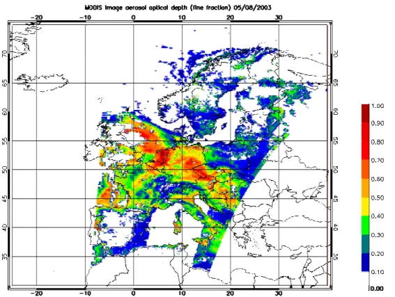
0.72 01 . 0 90 . 0 72 . 0 / 0.47 66 . 0 − ° − Θ − − = ρo ρo ηFigure 3.1 MODIS aerosol optical thickness (fine fraction) measured by the Terra satellite on 5 August 2003. Simulations with a chemistry-transport model for this day show that the high aerosol loading over the Netherlands and the North-Sea is caused by forest-fires in Portugal, which are advected over the Atlantic and the UK at an altitude of 3-4 km (Hodzic et al., 2005).
In this study, also the meteo-scaled optical thicknesses from the AOT and AOT were calculated. These are designated by AOT* and AOTF*, respectively. Data of the boundary
layer height and relative humidity at the surface were obtained from the ECMWF data archive. The three-hourly ECMWF data were interpolated in time and space to coincide with the MODIS overpass time.
3.2
Particulate matter concentrations from AirBase
Since the adoption of the EU air quality directives for particulate matter (EU, 1996; 1999), mass concentration measurements in Europe are performed operationally for particles smaller than 10 µm in diameter (PM10). In the past few years, also more and more measurement sites
are emerging for particles smaller than 2.5 µm in diameter (PM2.5), as these are suspected to
be more relevant for public health and therefore new air quality standards for PM2.5 have
been proposed by the European Commission to complement the PM10 standards.
These PM data are submitted to the AirBase data of the European Topic Centre on Air and Climate Change (ETC-ACC) of the European Environment Agency (EEA). This database consists of hourly or daily averaged values of PM, and meta-data, such as the latitude and longitude coordinates of the station, altitude, and information on its surroundings (urban background, (sub)urban background, street, industrial), measurement technique, etc.
Measurement techniques
The EU reference method to measure PM10 concentrations is described in CEN standard EN
12341, adopted by CEN in November 1998 (EN 12341, 1998). It defines a PM10 sampling
inlet coupled with a filter substrate and a regulated flow device. The mass collected on the filter is determined gravimetrically by means of a microbalance under well-defined environmental conditions. This is the reference method under the First Daughter Directive; it gives, by definition, the ‘correct’ PM10 results.
However, for practical reasons (requirement of technique to be fully automatic), also other methods can be used if a Member State can demonstrate that it gives equivalent results or displays a consistent relationship to the reference method. In the latter case, results have to be corrected by a correction factor to produce results equivalent to the reference method. These correction factors can vary substantially in space and even seasonally. Differences between correction factors and the application itself hinder integration on a European scale of all PM10
data. An overview of correction factors used for PM10 data of 2002 in the AirBase database is
given in Buijsman and de Leeuw (2004).
No European Reference Method for the measurement of the PM2.5 fraction has been
established up to now. Such a standard is currently being developed by CEN (CEN TC 264/Working Group 15) under a mandate of the European Commission. As for PM10, the
method is based on the gravimetric determination of the PM2.5 fraction of particles in the air,
sampled at ambient conditions. Also, for PM2.5 fully automatic techniques are used. At
present, no overview of applied correction factors for PM2.5 exists.
At this moment, the most commonly used techniques for measuring PM are gravimetry (i.e., the reference method), the beta-absorption technique and the Tapered Element Oscillating Microbalance (TEOM) technique.
• The gravimetry method is based on directly weighing the collected aerosols. Ambient air is pumped with a constant flow rate into a specially shaped inlet where particulate matter is separated into size fractions. The particulate matter is then collected on a filter and weighed in a temperature and humidity controlled environment.
• With the beta-absorption technique the amount of particles on the filter is determined by measuring the attenuation of a beam of beta-radiation (electrons) which are send through the filter. The attenuation is proportional to the mass of the aerosols on the filter.
• The TEOM makes use of the change in eigen-frequency of a tapered glass element that is connected to the filter. The change in eigen-frequency is determined by the mass of particles attached to the filter.
Measurement of PM mass concentrations are subject to considerable uncertainties mainly because of alterations of the air sample during the measurement process. Alteration of the air sample highly depends on the environmental conditions and composition of the particles. Loss of semi-volatile particles is the major problem. In most cases the results from beta-absorption instruments as well as the TEOM underestimate the concentration (e.g. Hitzenberger et al., 2004; Charron et al., 2004). The comparability of the PM mass measurements of these samplers has therefore been recognized as a major issue of concern (CAFE-WGPM, 2004).
Measurement locations
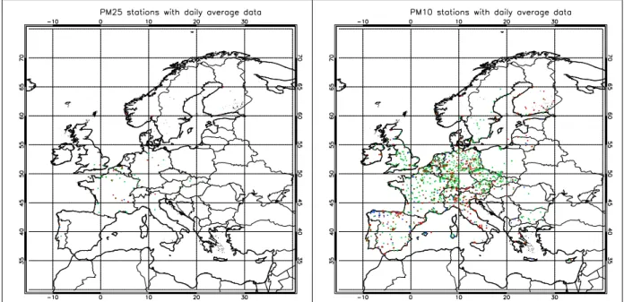
The PM measurement stations are located in different surroundings. Most stations are representative for background conditions in rural, sub-urban and urban areas. These are typically representative for areas of several km2 or larger. Also, there are many ‘Traffic’ stations, representative of concentration levels in streets and hence for a more limited area (scale of several tens of meters). A map of stations is presented in Figure 3.2.
Figure 3.2 Map of AirBase stations with daily average data of PM2.5 (left) and PM10 (right)
in 2003. Red: Traffic stations; Green: Background stations; Blue: Other, which include industrial stations, and stations for which the surroundings are not reported.
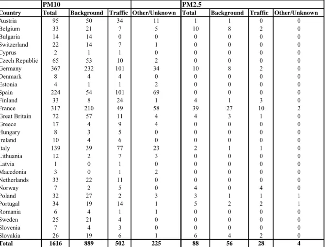
In 2003, 28 European countries submitted their PM10 data and 11 countries their PM2.5 data to
AirBase, see Table 3.1. Most stations only deliver daily averaged PM concentrations to Airbase. From the 88 PM2.5 stations that delivered daily average data, 23 stations also
delivered hourly data. The meta-information in AirBase includes a description of the surroundings (rural, suburban of urban), the type of station (traffic, background, or other), the measurement method used, the altitude etc. In Table 3.1 also a division into the two main types of stations, namely traffic and background is presented.
A number of elementary quality checks have been done on the AirBase data, such as removing data from stations with clearly erroneous latitude/longitude coordinates.
Table 3.1 Number of PM10 and PM2.5 measurement stations per country.
PM10 PM2.5
Country Total Background Traffic Other/Unknown Total Background Traffic Other/Unknown
Austria 95 50 34 11 1 1 0 0 Belgium 33 21 7 5 10 8 2 0 Bulgaria 14 14 0 0 0 0 0 0 Switzerland 22 14 7 1 0 0 0 0 Cyprus 2 1 1 0 0 0 0 0 Czech Republic 65 53 10 2 0 0 0 0 Germany 367 232 101 34 10 8 2 0 Denmark 8 4 4 0 0 0 0 0 Estonia 4 1 1 2 0 0 0 0 Spain 224 54 101 69 0 0 0 0 Finland 33 8 24 1 4 1 3 0 France 317 210 49 58 39 27 10 2 Great Britain 72 57 11 4 4 3 1 0 Greece 17 4 9 4 0 0 0 0 Hungary 8 3 5 0 0 0 0 0 Ireland 10 4 6 0 0 0 0 0 Italy 139 39 77 23 2 1 1 0 Lithuania 12 2 7 3 0 0 0 0 Latvia 1 0 1 0 0 0 0 0 Macedonia 3 0 1 2 0 0 0 0 Netherlands 33 22 11 0 0 0 0 0 Norway 7 2 5 0 4 0 4 0 Poland 32 27 2 3 3 1 1 1 Portugal 34 19 14 1 5 2 2 1 Romania 6 4 1 1 0 0 0 0 Sweden 25 21 4 0 0 0 0 0 Slovenia 7 4 3 0 0 0 0 0 Slovakia 26 19 6 1 6 4 2 0 Total 1616 889 502 225 88 56 28 4
In Table 3.2, an overview is given of measurement methods used for PM10 and PM2.5.
Clearly, most PM2.5 measurements are performed with the TEOM, whereas most PM10
measurements are performed with the beta-absorption technique.
Table 3.2 Measurement method and station type of the measurement locations.
PM2.5 PM10 Measurement method Oscillating Microbalance 57 484 Gravimetry 15 284 Beta-absorption 12 604 Other/Unknown 4 244 Stationtype (Sub-)urban background 40 650 Rural background 8 187 Traffic 28 502 Other 12 277
4.
Data assimilation system of LOTOS-EUROS
In this chapter, an overview is given of the LOTOS-EUROS model (Section 4.1) and the data-assimilation system (Section 4.2).
4.1
Modelling PM and AOT in LOTOS-EUROS
DomainThe master domain of LOTOS-EUROS is bound at 35° and 70° North and 10° West and 60° East. The projection is normal longitude-latitude and the standard grid resolution is 0.50° longitude x 0.25° latitude, approximately 25x25 km2. In this study, several domains within this master domain were considered. The final results are calculated over a domain that covers Europe (up to 40° East) but excludes the largest part of European Russia. In the vertical there are three dynamic layers and an optional surface layer. The model extends in vertical direction 3.5 km above sea level. The lowest dynamic layer is the mixing layer, followed by two reservoir layers. The height of the mixing layer is part of the diagnostic meteorological input data. The heights of the reservoir layers are determined by the difference between the mixing layer height and 3.5 km. Both reservoir layers are equally thick with a minimum of 50m. In some cases when the mixing layer extends near or above 3500 m the top of the model exceeds the 3500 m according to the abovementioned description. Simulations were performed with the optional surface layer of a fixed thickness of 25 m. Hence, this layer is always part of the dynamic mixing layer. For output purposes the concentrations at measuring height (usually 3.6 m) are diagnosed by assuming that the flux is constant with height and equal to the deposition velocity times the concentration at height z.
Transport
The transport consists of advection in 3 dimensions, horizontal and vertical diffusion, and entrainment/detrainment. The advection is driven by meteorological fields (u,v) which are input every 3 hours. The vertical wind speed w is calculated by the model as a result of the divergence of the horizontal wind fields. The recently improved and highly-accurate, monotonic advection scheme developed by Walcek (2000) is used to solve the system. The number of steps within the advection scheme is chosen such that the courant restriction is fulfilled. Entrainment is caused by the growth of the mixing layer during the day. Each hour the vertical structure of the model is adjusted to the new mixing layer thickness. After the new structure is set the pollutant concentrations are redistributed using linear interpolation. The horizontal diffusion is described with a horizontal eddy diffusion coefficient following the approach by Liu and Durran (1977). Vertical diffusion is described using the standard Kz-theory. Vertical exchange is calculated employing the new integral scheme by Yamartino et al. (2004).
Chemistry
The LOTOS-EUROS model contains two chemical mechanisms, the TNO CBM-IV scheme (Schaap et al., 2005a) and the CBM-IV by Adelman (1999). In this study, the TNO CBM-IV scheme is used, which is a modified version of the original CBM-IV (Whitten et al., 1980). The scheme includes 28 species and 66 reactions, including 12 photolytic reactions. Compared to the original scheme steady state approximations were used to reduce the number of reactions. In addition, reaction rates have been updated regularly. The mechanism
was tested against the results of an intercomparison presented by Poppe et al. (1996) and found to be in good agreement with the results presented for the other mechanisms. Aerosol chemistry is represented using ISORROPIA (Nenes et al., 1999).
Dry and wet deposition
The dry deposition in LOTOS-EUROS is parameterised following the well known resistance approach. The deposition velocity is described as the reciprocal sum of three resistances: the aerodynamic resistance, the laminar layer resistance and the surface resistance. The aerodynamic resistance is dependent on atmospheric stability. The relevant stability parameters (u*, L and Kz) are calculated using standard similarity theory profiles. The
laminar layer resistance and the surface resistances for acidifying components and particles are described following the EDACS system (Erisman et al., 1994).
Below cloud scavenging is described using simple scavenging coefficients for gases (Schaap et al., 2004) and following Simpson et al. (2003) for particles. In-cloud scavenging is neglected due to the limited information on clouds. Neglecting in-cloud scavenging results in too low wet deposition fluxes but has a very limited influence on ground level concentrations (see Schaap et al., 2004).
Meteorological input
The LOTOS-EUROS system is presently driven by 3-hourly meteorological data. These include 3D fields for wind direction, wind speed, temperature, humidity and density, substantiated by 2-dimensional gridded fields of mixing layer height, precipitation rates, cloud cover and several boundary layer and surface variables. The standard meteorological data for Europe are produced at the Free University of Berlin employing a diagnostic meteorological analysis system based on an optimum interpolation procedure on isentropic surfaces. The system utilizes all available synoptic surface and upper air data (Kerschbaumer and Reimer, 2003). Also, meteorological data obtained from ECMWF can be used to force the model.
Emissions
The anthropogenic emissions used in this study are a combination of the TNO emission database (Visschedijk et al., 2005) and the CAFE baseline emissions for 2000. For each source category and each country, the country totals of the TNO emission database were scaled to those of the CAFE baseline emissions. Elemental carbon (EC) emissions were derived from (and subtracted from) the primary PM2.5 (PPM2.5) emissions following Schaap
et al. (2004b). Hence, the official emission totals were used as used within the LRTAP protocol, but also the benefit are exploited from the higher resolution of the TNO emission database (0.25x0.125 lon-lat). The annual emission totals are broken down to hourly emission estimates using time factors for the emissions strength variation over the months, days of the week and the hours of the day (Builtjes et al., 2003).
In LOTOS-EUROS biogenic isoprene emissions are calculated following Veldt (1991) using the actual meteorological data. In addition, sea salt emissions are parameterised following Monahan et al (1986) from the wind speed at ten meter height. Dust was neglected as it normally does not contribute a large fraction to the fine aerosol mass in Europe and, more importantly, because there are no reliable emission estimates and/or parameterisations
Boundary conditions
The boundary conditions for ozone are derived from the 3-dimensional tropospheric ozone climatology by Logan (1998), which is derived from ozone sonde data. For a number of components, listed in Table 4.1 the EMEP method is followed (Simpson et al., 2003) based on measured data. In this method simple functions have been derived to match the observed distributions. The boundary conditions are adjusted as function of height, latitude and day of the year. The functions are used to set the boundary conditions, both at the lateral boundaries as at the model top. The annual cycle of each species is represented with a cosine-curve, using the annual mean near-surface concentration, C0, the amplitude of the cycle ΔC, and the
day of the year at which the maximum value occurs, dmax. Table 4.1 lists these parameters.
First the seasonal changes in ground-level boundary condition, C0, are calculated through:
⎟ ⎟ ⎠ ⎞ ⎜ ⎜ ⎝ ⎛ − ⋅ Δ + = y mm mean n d d C C C cos 2 ( max) 0 π
where ny is the number of days per year, dmm is the day number of mid-month (assumed to be
the 15th), and dmax is day number at which C0 maximizes, as given in Table 4.1. Changes in
the vertical are specified with a scale-height, Hz, also given in Table 4.1.
Hz h i h C e
C ( )= 0 −
where Ci(h) is the concentration at height h (in km). For simplicity h is set to be the height of
the centre of each model layer assuming a standard atmosphere. For some species a latitude factor, given in Table 4.2, is also applied. Values of Ci adjusted in this manner are
constrained to be greater or equal to the minimum values, Cmin, given in Table 4.1. Ammonia
boundary conditions are neglected. Sulphate is assumed to be fully neutralized by ammonium. Nitrate values are assumed to be included in those of nitric acid and are zero as well.
Table 4.1 Parameters used to set the boundary conditions
Parameter Cmean dmax ΔC Hz C0min
min h C ppb days ppb km ppb ppb SO2 0.15 15.0 0.05 ∞ 0.15 0.03 SO4 0.15 180.0 0.00 1.6 0.05 0.03 NO 0.1 15.0 0.03 4.0 0.03 0.02 NO2 0.1 15.0 0.03 4.0 0.05 0.04 PAN 0.20 120.0 0.15 ∞ 0.20 0.1 HNO3 0.1 15.0 0.03 ∞ 0.05 0.05 CO 125.0 75.0 35.0 25.0 70.0 30.0 ETH 2.0 75.0 1.0 10.0 0.05 0.05 FORM 0.7 180.0 0.3 6.0 0.05 0.05 ACET 2.0 180.0 0.5 6.0 0.05 0.05
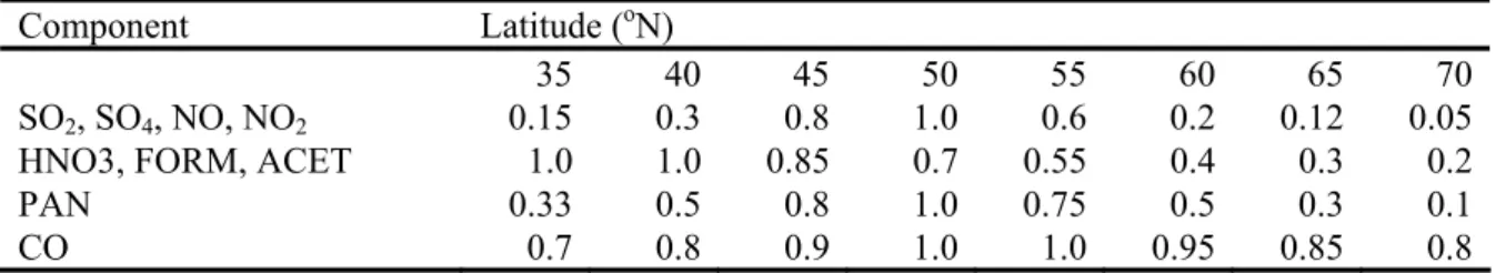
Table 4.2 Latitude factors applied to the prescribed boundary conditions
Component Latitude (oN)
35 40 45 50 55 60 65 70
SO2, SO4, NO, NO2 0.15 0.3 0.8 1.0 0.6 0.2 0.12 0.05
HNO3, FORM, ACET 1.0 1.0 0.85 0.7 0.55 0.4 0.3 0.2
PAN 0.33 0.5 0.8 1.0 0.75 0.5 0.3 0.1
CO 0.7 0.8 0.9 1.0 1.0 0.95 0.85 0.8
AOT calculation
The AOT is computed from the dry aerosol mass concentrations derived from the LOTOS-EUROS model using the approach of Kiehl and Briegleb (1993):
AOTi(λ) = f (RH, λ) * ai(λ) * Bi (λ)
where ai(λ) is the mass extinction efficiency of the compound i; Bi is the column burden of
the compound i; f (RH, λ) is a function describing the variation of the scattering coefficient with relative humidity (RH) and wavelength (l). To compute ai(λ) for dry inorganic particles,
a Mie (Mie, 1908) code has been used, assuming the aerosol size distribution to be log-normal, with a geometric mean radius of 0.05μm, a geometric standard deviation of 2.0 and a sulphate dry particle density of 1.7 g cm−3 (Kiehl and Briegleb, 1993). Most aerosol particles absorb or release water vapour when the relative humidity (RH) changes. Thus the size and composition of the particles change, resulting in different light scattering properties. To account for the variation of the aerosol scattering coefficient with RH, the factor f(RH, λ), derived from humidity controlled nephelometry (Veefkind et al., 1996), is used (see Figure 2.2). Similar functions for f(RH) have been reported by Day et al. (2001) for various locations in the United States. Effects due to hysteresis (e.g. Tang, 1997) are not accounted for. The wavelength dependence of f (RH) can be ignored (Veefkind et al., 1999). The scattering calculations were made with RH values taken from the analysed meteorological data file that is used as input to the LOTOS-EUROS model, including the variations of RH with height. For the organic aerosol components an ai of 9 for EC and 7 for OC is assumed
(Tegen et al., 1997). For these components the growth as function of RH has been neglected.
4.2
Ensemble Kalman filter
The first step in order to build the Ensemble Kalman Filter around LOTOS-EUROS is to embed the model and the available measurement in a stochastic environment:
xk+1 = fk(xk,wk)
yk = Ckxk + vk,
where the superscripts (k) denote the time-steps. The model state vector is denoted by x and
the measurements by y. The function f denotes the non-linear model operator which apart
from on the state vector acts on a white noise vector w with Gaussian distribution and
diagonal covariance matrix Q. The measurement vector y is assumed be a linear combination
of elements of the state vector and a random, uncorrelated Gaussian error v with (diagonal)
covariance matrix R. The basic idea behind the ensemble filter is to express the probability
function of the state in an ensemble of possible states {ξ1,..., ξN}, and to approximate
∑
= ≈ N j j N x 1 1 ˆ ξ(
)(
)
T j N j j x x N P ˆ ˆ 1 1 1 − − − ≈∑
= ξ ξwhere the pair ( xˆ ,P) (expectation and covariance matrix) describe the probability of the state vector x completely if x has a Gaussian distribution. Since the models are strongly non-linear, it cannot be expected that x really has a Gaussian distribution. It is assumed however that the distribution is at least close to Gaussian so that the bulk of the statistical properties is captured by the pair ( xˆ ,P). The filter algorithm consists of three stages:
initialisation:
each ensemble member is set to the initial state:
0
x
j =
ξ
forecast:
each ensemble member is propagated in time by the model, where the noise input wk is drawn from a random generator with covariance Q;
) , ( k j f j f ξ w ξ = analysis:
given an (arbitrary) gain matrix K, each ensemble member is updated according to:
) ( f j T f j a j ξ K y ν H ξ ξ = + + −
where ν represents a measurement error, drawn from a random generator with zero mean and covariance R. The gain matrix K is given by the optimal gain matrix from the original Kalman Filter. In the original filter the Kalman gain was obtained by matrix multiplications in which the covariance matrix P is involved. Fortunately, the use of this matrix can be avoided, since this matrix is too large to store into memory. Instead, a square root S (such that P=SST) can be used. From the definition of P it can be seen that the columns si of such a
square root can be defined by
(
x)
N si i ˆ 1 1 − − = ξ .Note that the sample mean xˆ , and the matrix S completely define the ensemble and vice versa; it is therefore not necessary to store both S and the ensemble. The analysis of the measurements yj (entries of the vector y) can now be performed by the following sequential
(
)
(
)
(
1)
1 1 1 1 1 1 1 − − − − − − − − + = − = = + = + = = j j j j j j T j j j j j j j j j jj j j jj j T j j T j T j j x c y h x x h k b S S h S a k r a b r h h a c S hThe index j is the iteration index. The starting values for the procedure are 0 = +1
k f S S and 1 0 + = k f x
x . After the analysis of all the measurements the final values for the state vector and
(square root of) the covariance matrix have been obtained: m
k S S +1= and m k x x +1= . For a detailed description, reference is made to Van Loon et al. (2000) and Evensen (1997).
The forecast step is the most expensive part of the algorithm, since for each ensemble member the model has to be evaluated one time. Typical ensemble sizes range from 10-100. If the number of measurements is limited (in order of hundreds), the total computation time involved with the ensemble filter is proportional with the ensemble size.
Random noise
In the model implementation used in this study, the noise parameters are part of the model state. Hence they are estimated by the filter as well. In Chapter 7, the noise to several emission fields Ej is specified. The noise parameters wi can be interpreted as emission
correction factors since the actual emission field Ej is estimated by the filter as
Ei ← Ej (1+wi).
This approach has the disadvantage that there is no ‘memory’ in the system: the wi are
uncorrelated in time; at a certain hour t the noise parameter may indicate an emission increase of 20% with respect to the original field, whereas it estimates a decrease of 20% at t+1. Such irregular behaviour can be prevented to a large extent by the use of coloured noise. However, in the present set-up, the same noise factors for the 24 hour period between overpasses were used. Hence, the long period between the measurements warrants some correlation in time.
Spatially limiting influence of measurements
For two reasons correlations between elements in the state vector arise which are unlikely to be correlated. Firstly, spurious correlations arise, mainly because the sample size is finite. Secondly, undesired correlations arise due to the choice of the noise processes. The noise processes to be introduced in this study are all acting on emission fields of various emitted compounds causing ‘instantaneous’ correlations throughout the domain. For example the particulate matter concentration at hour t somewhere in The Netherlands becomes correlated with the particulate matter concentration in, say, the south of France, because noise was added to the NOx emission field at hour t-1. Although this is exactly what should happen
when defining noise in this way, such correlations are not realistic and should be somehow ignored by the filter. The noise processes is chosen this way because it is infeasible to subdivide the emission fields into a number of sub-domains on each of which a different noise parameter is acting. That would increase the dimension of the noise vector dramatically and hence the necessary ensemble size to capture the statistical properties.
One way to ignore unrealistic correlations over large distances is the use of a gain matrix which is only unequal to zero around the locations of observations. Such a gain matrix k may be formed using a covariance matrix which is an element wise product of the original sample covariance and a correlation function with local support. For a single scalar measurement, the resulting gain matrix is given by (omitting the subscripts):
) /( ) ( Ph h Ph r I k = ρ T +
where I(ρ) is a diagonal matrix; the diagonal elements are filled with a prescribed correlation
between the corresponding grid cell and the grid cell of the measurement. Different choices for the values of ρi are possible. In this study it is assumed that
ρ i = exp(-0.5 (ri/L)2) for ri ≤ 3.5 L
and zero otherwise. ri denotes the distance from the grid cell considered to the site of the
analysed measurement and L denotes a length scale parameter, taken to be 100 km in this study.
5.
Validation of MODIS AOT using AERONET
5.1
Analysis of yearly average data
AERONET is an optical ground based aerosol monitoring network supported by NASA’s Earth Observing System and other international institutions. It consists of identical automatic sun-sky scanning spectral radiometers. The network provides, among others, globally distributed observations of aerosol optical thickness. In previous studies, the retrieved AOT has been validated against a limited set of AOT measurements from the ground-based AERONET network on a global scale. These validations showed that the retrieved AOT is generally within the pre-specified accuracy of ±0.05±0.20AOT over land and ±0.03±0.05AOT over oceans (1-σ level, for individual retrievals), except in situations with possible cloud contamination, over surfaces with sub pixel surface water such as coastal areas and over surfaces with sub pixel snow cover (Chu et al., 2002; Ichoku et al., 2005). In this study, MODIS AOT and AOTF were validated against AERONET observations of in more
detail for Europe in 2003.
-0.1 0.0 0.1 0.2 0.3 0.4 Blid a Mins k Oo st en de T ora ve re Av ig no n Bo rd eau x D unk er qu e Fo nt ai ne bl eau Lille Ros sf eld To ul ou se Pa la is ea u Ha m bu rg He lg ol an d IF T-Le ip zi g M un ich M ai sach Fo rt h C re te Et na IM C O ris ta no IS D G M _C N R Is pr a La m pe du sa L ecce U ni ver si ty R om e T or Ve rg at a Ve ni se Mo ldo va Th e H ag ue Be ls k Ca bo da R oc a Ev or a Mo sc ow MS U MO E l A re nos illo Pa le nc ia G otla nd L aeg er en IM S-M ETU -E R D EM L I O b se rvat io n s
MODIS AOT minus Aeronet AOT MODIS AOTF minus Aeronet AOT
Figure 5.1 Difference between AERONET AOT and MODIS AOT (and AOTF) at AERONET
stations.
For our validation exercise all 36 AERONET stations that provided data for 2003 in Europe were used. Figure 5.1 shows the difference in the absolute values of MODIS and AERONET AOT for the individual stations. It is evident from Figure 5.1 and Table A.1 (Annex 1) that MODIS generally overestimates the AOT values measured by AERONET at almost all the stations. The difference is variable for the different stations. On average, the annual mean AOT and AOTF observed by MODIS across all stations are 0.30 and 0.25 respectively, while
that observed at AERONET stations is 0.20, providing a mean annual difference of 0.10 for AOT and 0.05 for AOTF across all stations. For western Europe, the extent of the
overestimation by MODIS is in agreement with findings from Remer et al. (2005).
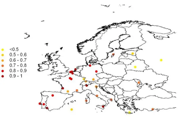
Besides average differences, also the spatial correlation of yearly average optical thicknesses were considered. This is particularly important, as the spatial gradients of yearly average AOT play an important role if the AOT is used for improvement of mapping yearly average PM levels. It was found that the spatial correlation between AERONET AOT and MODIS is 0.64 for the AOT and 0.72 for the AOTF.
5.2
Analysis of time-series per station
Figure 5.2 Time correlations between AOT from AERONET and MODIS.
0.0 0.2 0.4 0.6 0.8 1.0 Al ge ri a Bel ar us Be lgiu m Es to ni a Fr an ce Fr an ce Fr an ce Fr an ce Fr an ce Fr an ce Fr an ce Fr an ce Ge rm an y Ge rm an y Ge rm an y Ge rm an y G reece Ital y It al y It al y It al y It al y It al y It al y It al y Mo ldo va N ethe rla nd s Po la nd Po rt ug al Po rt ug al Ru ss ia Sp ai n Sp ai n Sw ed en Sw itz er la nd Tu rk ey C o rrela ti o n
Correlation Aeronet-MODIS AOT Correlation Aeronet-MODIS(AOTF)
Figure 5.3 Time correlations between AERONET AOT and MODIS AOT (AOTF).
The temporal correlations between the MODIS and AERONET at the AEORNET stations are presented in Figures 5.2 and 5.3 and are also listed in Table A.1 (Annex 1). The time-series of MODIS and AERONET AOT show a correlation of 0.72, averaged over all stations. The median of the correlation coefficients is 0.77. For MODIS AOTF versus AERONET AOT,
these correlations are slightly lower. This is understandable, since the AOTF only pertains to
the optical thickness due to the smaller particles. Indeed, particularly in Southern Europe, (southern Italy, Portugal and Spain), the correlations with AOTF are sometimes much lower
than those with the AOT. This might point at a high contribution of coarse particles to the AOT. This is consistent with the fact that the difference between yearly average AOT and AOTF observed by MODIS is large at these stations. Poor correlation coefficients are found
for stations with sparse data (e.g, Belsk, Poland). Stations with less than 15 days with simultaneous measurements have therefore been removed from the analysis.
Avignon 0.0 0.2 0.4 0.6 0.8 1.0 0 50 100 150 200 250 300 350 Julian Day (2003) AO D
AERONET MODIS MODIS(AODF)
a) ISDGM-CNR 0.0 0.2 0.4 0.6 0.8 1.0 1.2 1.4 0 50 100 150 200 250 300 350 Julian Day (2003) AO D
AERONET MODIS MODIS(AODF)
b) Lampedusa 0.0 0.2 0.4 0.6 0.8 1.0 150 200 250 300 350 Julian Day (2003) AO D
AERONET MODIS MODIS(AODF)
c)
Figure 5.4 Temporal variation of AERONET AOT and MODIS AOT and AOTF at a)
In general, MODIS AOT and AOTF exhibit a similar seasonal variation to that observed at
AERONET stations. Examples are given in Figure 5.4 for Avignon (France), ISDGM-CMR (Italy), and Lampedusa (Italy, in the Mediterranean sea) . Generally high AOT (AOTF) values
are being observed in summer and low AOT (AOTF) values in winter. The MODIS AOT,
however, exhibits a stronger seasonal trend than AERONET AOT. The difference between MODIS and AERONET AOT and AOTF is summarized for all sites in Figure 5.5. In winter
and summer average residuals for AOT (AOTF) are 0.05 (0.01) and 0.16 (0.10), respectively.
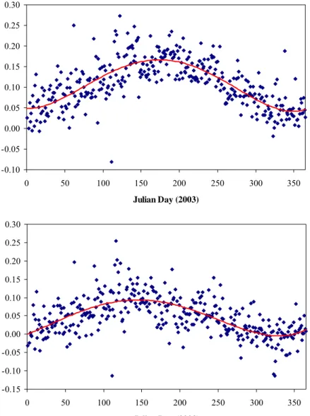
In a relative sense, the difference remains practically constant throughout the year (see Figure 5.6). On the whole, the AERONET AOT is about 70% of MODIS AOT and 90% of MODIS AOTF. -0.10 -0.05 0.00 0.05 0.10 0.15 0.20 0.25 0.30 0 50 100 150 200 250 300 350 Julian Day (2003) M O D IS A O T m inus A e rone t A O T a) -0.15 -0.10 -0.05 0.00 0.05 0.10 0.15 0.20 0.25 0.30 0 50 100 150 200 250 300 350 Julian Day (2003) M O D IS A O TF m inus A e rone t A O T b)
Figure 5.5 a) Seasonal variation of the absolute difference between MODIS and AERONET AOT for all sites averaged; b) Same as (a), but for the AOTF from MODIS.
0.0 0.5 1.0 1.5 2.0 0 50 100 150 200 250 300 350 Julian Day (2003) Ae ro n e t AO T : M O D IS AO T a) 0.0 0.5 1.0 1.5 2.0 0 50 100 150 200 250 300 350 Julian Day (2003) A e rone t A O T : M O D IS A O TF b)
Figure 5.6 a) Relative difference between MODIS and AERONET AOT for all sites averaged, and b) Same as (a), but for the AOTF from MODIS.
It was investigated whether the MODIS AOT is as accurate (1-sigma error ±0.05±0.20AOT) as claimed in the literature. Table 5.1 summarises the percentage of MODIS retrievals for which the AERONET observation is within 1 or 2 sigma from the MODIS retrieval. From a statistical point of view, and assuming normally distributed data, 66% of the data should be within the 1-sigma and 95% within the 2-sigma range. The MODIS AOT does not fulfil this requirement, which is attributed to the relatively high bias in these data. After correction for the bias (simply by multiplication AOT data with 0.7, and AOTF data with 0.9), the MODIS
accuracy agrees within 1-sigma limits ±0.05±0.20AOT. The frequency distributions of the bias-corrected difference between AERONET and MODIS are shown in Figure 5.7.
Table 5.1 Percentage of MODIS retrievals for which the AERONET observation is within 1 or 2 sigma from the MODIS retrieval, where sigma = ±0.05± 0.20AOT.
% within 1-sigma % within 2-sigma
AOT 55 91
AOT* 0.7 73 96
AOTF 64 93
AOTF * 0.9 68 93
Figure 5.7 Frequency distributions of the difference between AERONET and MODIS (bias corrected). Top: AERONET versus MODIS AOT, Bottom AERONET versus MODIS AOTF.