Probabilistic modeling of dietary intake of substances - The risk management question governs the method

(1)

RIVM report 320011001/2005

Probabilistic modeling of dietary intake of substances

The risk management question governs the method MN Pieters, BC Ossendorp, MI Bakker, W Slob

Contact: Moniek Pieters

Centre for Substances and Integrated Risk Assessment

MN.Pieters@rivm.nl

This investigation has been performed by order and for the account of the Ministry of Welfare and Sports, within the framework of project 320011, Risk assessment of food.

(2)

Abstract

Probabilistic modeling of dietary intake of substances. The risk management question governs the method.

In this report the discussion on the use of probabilistic modeling in relation to pesticide use in food crops is analyzed. Due to different policy questions the current discussion is complex and considers safety of an MRL as well as probability of a health risk. The question regarding the use of ‘consumers only’ data versus ‘total population’ is addressed in the light of the policy questions at stake. We distinguish four domains in the dietary exposure assessment that require a different probabilistic approach, based on the following two distinctions: long-term vs. acute exposure assessment, and frequently vs. incidentally consumed products. With a recently developed model at RIVM probabilistic modeling can now be performed for long-term ánd acute dietary intake in the case of frequently ánd incidentally eaten foods. Modeling the intake for more than one food is, at this stage, only possible for assessing long-term dietary intake where zero daily (total) intakes are rare.

(3)

Rapport in het kort

Probabilistische berekening van de inname van stoffen via de voeding. De beleidsvraag bepaalt de methode.

Probabilistische modellering voor het berekenen van de inname van bestrijdingsmiddelen via de voeding heeft het voordeel dat onnodig conservatieve schattingen worden voorkomen. De toepassing van probabilistische modellering vereist echter dat verschillende

beleidsbeslissingen expliciet moeten worden genomen. Deze betreffen de fractie van de bevolking die beschermd moet worden én de acceptabele fractie van dagen met

overschrijding. Dit rapport analyseert de verschillende beleidsvragen die leiden tot een innameberekening uit voedsel. De eerste betreft de veiligheid van elk voedingsmiddel, de tweede het risico van een partij met te hoog residugehalte en de derde beleidsvraag gaat in op het gezondheidsrisico bij werkelijke blootstelling. Innameberekeningen worden bemoeilijkt doordat de informatie die in de Nederlandse Voedselconsumptie Peiling (VCP) beperkt is en bewerkt moet worden voordat deze te gebruiken is. Getoond wordt dat de beleidsvraag bepalend is voor de manier waarop een innameberekening dient te worden uitgevoerd. Het berekenen van de lange-termijn inname van voedingsmiddelen die veel worden gegeten was al langer mogelijk. Met behulp van een recent op het RIVM ontwikkeld model zijn

probabilistische innameberekeningen nu ook mogelijk voor voedingsmiddelen die incidenteel worden gegeten. Ook kan de korte-termijn inname (1 dag) worden berekend. Het berekenen van de inname van bestrijdingsmiddelen via meerdere voedingsmiddelen is alleen nog maar mogelijk voor de lange-termijn inname van frequent gegeten voedingsmiddelen.

(4)

Samenvatting

De risicoschatting van stoffen omvat een schatting van blootstelling en van effect. Humane grenswaarden zoals een ADI, TDI, ARfD zijn gebaseerd op toxicologische gegevens en inzichten en inname beneden deze grenswaarden wordt als ‘veilig’ beschouwd voor alle individuen in de populatie. Productlimieten zoals maximum residu limieten (MRL) voor pesticiden op voedingsmiddelen zijn gebaseerd op andere overwegingen: de toepassing van een pesticide op gewassen volgens ‘Good Agricultural Practice’ in gecontroleerde

veldexperimenten. Door de inname van pesticiden via voedingsmiddelen te berekenen en te vergelijken met een humane grenswaarde, wordt bepaald of een MRL ook veilig is. Doordat de berekende acute inname van pesticiden in veel gevallen de Acute Reference Dose (ARfD) overschreed en Codex MRLs hierdoor niet konden worden vastgesteld, ontstond een

internationale discussie over het gebruik van probabilistische modellering voor het berekenen van de inname. Bij probabilistische modellering worden verdelingen van variabelen in plaats van (vaak worst case) puntschattingen hiervan gecombineerd. Dit rapport analyseert de internationale discussie met betrekking tot probabilistische modellering voor pesticiden in voedingsmiddelen. Deze internationale discussie is complex omdat er drie beleidsvragen spelen. De eerste beschouwt de veiligheid van elk voedingsmiddel. Is er een

gezondheidsrisico wanneer een voedingsmiddel met residuen op de MRL wordt geconsumeerd? De tweede vraag beschouwt het risico van een partij met een residuconcentratie die hoger is dan de MRL en de derde vraag gaat in op de

waarschijnlijkheid dat een gezondheidsrisico werkelijk zal optreden. Voor deze laatste vraag is de variatie in concentraties en in consumptie van belang. Het debat over het gebruik van consumptiedata van ‘consumers only’ of ‘total population’ kan worden beschouwd als een gevolg van deze verschillende vraagstellingen. Deze laatste discussie wordt gecompliceerd door een niet correct gebruik van terminologie en de afwezigheid van een eenduidige beleidsdefinitie van ‘veilig’.

In het rapport onderscheiden we vier domeinen van blootstelling via de voeding. Elk van deze domeinen dient op een andere probabilistische wijze benaderd te worden aangezien de informatie die benodigd is verschilt. Voor een schatting van de lange-termijn blootstelling is de gemiddelde residuconcentratie relevant, terwijl voor het schatten van de acute blootstelling de variatie in concentratie van belang is. Voor voedingsmiddelen die niet regelmatig gegeten worden is het niet alleen van belang om een verdeling van de geconsumeerde hoeveelheden te hebben, maar ook om de consumptiefrequenties van deze voedingsmiddelen te schatten. Dit laatste kan worden uitgevoerd met een model dat recent op het RIVM is ontwikkeld. We laten zien dat probabilistische modellering verschillende nieuwe inzichten kan bieden. Echter, een beleidsbeslissing omtrent de fractie van de populatie, bijvoorbeeld 95%, 99%, (of van een subpopulatie, bijvoorbeeld kinderen) die beschermd dient te worden tegen

gezondheidseffecten is noodzakelijk. Dit geldt ook voor welke kans van overschrijding van een ARfD door een individu nog als acceptabel wordt geacht. Probabilistische modellering van meerdere voedingsmiddelen is momenteel alleen mogelijk voor lange-termijn

(6)

Summary

The risk assessment of substances comprises exposure assessment and effect assessment. Human limit values such as ADI, TDI, ARfD are based on toxicological data, and intakes below these limits are considered to be ‘safe’ for (almost) every individual in the population. Product limits such as maximum residue limits (MRLs) for pesticides on commodities are based on other considerations, in particular, the application of a substance on crops using Good Agricultural Practice in supervised trials. By calculating the dietary intake of pesticides and comparing with a human limit value it is decided whether an MRL is safe. Since the calculated acute intake exceeded the Acute Reference Dose (ARfD) in many cases,

preventing establishment of Codex MRLs, an international debate was started on the use of probabilistic exposure modeling for estimating the dietary intake. With probabilistic modeling distributions of variables are combined instead of using (often worst case) deterministic (or point) values for these variables. This report analyzes the discussion on probabilistic modeling in relation to pesticide use in foods. The international discussion is complex since three policy management questions are at stake. The first considers the safety of the MRL. Is there a health risk when a food product with residues at the MRL is

consumed? The second question considers the health risk of a lot with residue concentrations higher than the MRL, while the third question addresses the probability that a health risk may really occur. For the latter question variation in concentrations and variation in consumption are important. The debate on using consumption data of either ‘consumers only’ or ‘total population’ can be considered as a spin off from these different risk management queries. This latter discussion is complicated by the use of incorrect terminology and the absence of a clear risk management definition of ‘safety’.

We distinguish four domains in the dietary exposure assessment. Each of these domains requires a different probabilistic approach since they differ in the information that needs to be extracted from the data. For long-term exposure an average residue concentration is relevant, while for acute exposure the variation in residue concentration is relevant as well. For

incidentally eaten foods not only the distribution of consumed amounts but also of consumption frequencies needs to be estimated. This can be done by a model recently developed at RIVM. We show that probabilistic modeling can offer risk managers various new insights. However, it requires a policy decision on the fraction, for example 95%, 99%, of the population (or, of a subpopulation, e.g., children) that should be protected against health effects. Also a decision should be made on which probability of exceeding an ARfD in a single individual is considered acceptable. Concerning probabilistic modeling on more than one food item we conclude that this is as yet only possible for long-term exposure, where total intake on a single day is rarely zero.

(7)

1. Introduction

The risk assessment of chemicals in food is often performed by comparing the dietary intake with a human limit value, such as ADI (acceptable daily intake) or TDI (tolerable daily intake) in the case of long-term exposure or an Acute Reference Dose (ARfD) in the case of acute exposure. The average dietary intake can be estimated by combining the average concentration of the chemical in relevant food products with the average consumption rates of these products. The use of average intake may be valuable when the estimated intake is far below human limit values. However, when the margin between average intake and human limit values is not that large, a more detailed exposure assessment is necessary. With probabilistic modeling distributions of variables are combined instead of using (worst case) deterministic (or point) values for these variables. This distributional approach prevents worst case assumptions from ‘piling up’ and will therefore not result in a high estimate with a very low probability of occurring, as is often the case with deterministic assessments.

Currently, in the process of establishing Maximum Residue Limits (MRLs), a deterministic exposure assessment is carried out. Experience with this procedure showed that the calculated short-term intake exceeded the Acute Reference Dose (ARfD) in many cases. Since this prevented Codex MRLs from being established an international debate was started on the worst case assumptions of the deterministic exposure assessment. In this debate probabilistic modeling was suggested as an alternative to estimate the intake in a more realistic way. This report elaborates on the current discussion on probabilistic modeling in relation to pesticide use in foods. Chapter 2 combines an analysis of the international discussion with the possibilities of probabilistic dietary exposure assessment. The subsequent chapters discuss probabilistic modeling in more detail and form the scientific basis of Chapter 2. We distinguish four domains in the dietary exposure assessment that call for a different

probabilistic modeling approach since they differ in the information that needs to be extracted from the data and we identify issues that risk managers should decide on.

(8)

2. Probabilistic modeling in relation to pesticide use

in food and feeding crops

2.1 Introduction

The MRL is the maximum concentration of a pesticide residue (expressed as mg/kg) to be legally permitted in or on food commodities and animal feed (FAO/WHO, 2000). Though registration of pesticides occurs at the national level, the Codex Committee on Pesticide Residues (CCPR) aims to establish world-wide harmonized Codex MRLs. Concerning the derivation of MRLs, the Codex formulated two goals:

1. Codex MRLs, are primarily intended to apply in international trade

2. Foods complying with the Codex MRLs should be safe for human consumption An MRL is based on a set of data of supervised field trials in which the crop is treated with a concentration of the pesticide equivalent to the ‘worst case’ use but within the limits of Good Agricultural practice (GAP). MRLs are expressed as mg residue (as defined) per kg raw agricultural commodity (RAC) on a fresh weight basis and are proposed at a concentration level higher than the highest residue found in supervised trials and taking into account the variation in the available data1. The enforcement of MRLs prevents unauthorized use of pesticides. Since an MRL is not based on toxicological considerations, the value of an MRL is not directly related to health considerations. However, to ensure that food items with pesticide concentrations at the MRL are safe for human consumption, the total intake of the pesticide via the diet is calculated and compared with the Acceptable Daily Intake (ADI) in the case of life-time exposure. If the total intake exceeds the ADI, a Codex MRL is not established. If a company wishes to obtain Codex MRLs for these pesticide-commodity combinations it has to (1) adjust the GAP and/or (2) provide new toxicological studies that may allow refinement of ADI/ARfD and/or (3) provide new residue data that may allow refinement of the intake assessment, e.g. processing data.

Since 1995 Acute Reference Doses (ARfD) are available for several pesticides, while exposure assessments based on short-term exposure are carried out as well (see Hamilton et

al., 2004 for an overview). The following definition of the ARfD was adopted by the 2002

JMPR: ‘The ARfD of a chemical is an estimate of the amount of a substance in food and/or drinking-water, normally expressed on a body-weight basis, that can be ingested in a period of 24 h or less, without appreciable health risk to the consumer, on the basis of all the known facts at the time of the evaluation’ The concept of the ARfD was developed by JMPR

(FAO/WHO, 2005) as a health safety limit aimed at preventing health risks. It is set to ensure that when the intake stays below this value no health risk is anticipated from acute exposures. However, the ARfD is also used by enforcement authorities, where the limit is more or less regarded as an intervention value. In this case, the limit is considered as a level above which health effects might start to occur. Ideally, the concept of the ARfD should be able to cover both needs indicating that exceeding ARfD should not be tolerated. With the use of

1_{Codex MRLs are derived from estimations made by the Joint WHO/FAO Meeting on Pesticides Residues}

(JMPR) following a) toxicological assessment of the pesticide and its residue; and b) review of residue data from supervised trials including those reflecting national good agricultural practices. The methods used by the JMPR to estimate maximum residue levels differ in some ways from those used by other bodies (e.g. the EU, the USA). The methods for deriving maximum residu limits (MRLs) and residu levels in risk assessment (supervised trial median residu (STMR) and Highest Residu (HR)) as described in this report all refer to the guidelines of the JMPR (FAO 2002).

(9)

probabilistic modelling it is necessary to define which low probability of exceeding the ARfD in an individual is considered acceptable.

As mentioned earlier, it turned out that the calculated short-term intake exceeded the ARfD in many cases, preventing establishment of Codex MRLs. An international debate was started on the use of probabilistic exposure modeling to obtain a more adequate (and less

conservative) estimate of the dietary intake (CCPR, 2002; CCPR, 2003; CCPR, 2004). Though this debate mainly focuses on the short-term exposure (acute exposure within 24 hours), we will discuss probabilistic modeling for both long-term and short-term exposure in depth in the subsequent chapters. In this chapter the insights relevant for the current

international debate are presented in more detail.

2.2 Current procedure of MRL derivation and deterministic

exposure assessment

Derivation of an MRL

Supervised residue trials are performed to obtain data on residue concentrations occurring after treating crops with pesticides in a worst case scenario but still within the limits of Good Agricultural practice (GAP). The trials are evaluated, yielding a subset of suitable trials. The highest residue found in these trials is used for the estimation of a maximum residue level, which can be used to establish a Codex MRL.

One has to bear in mind that an MRL is used to enforce proper use of the pesticide according to GAP. For that purpose analytical laboratories all over the world are doing lots of analyses. As many pesticide residues as possible are measured in one single analytical run (‘multi-residue methods’). Therefore, the (‘multi-residue definition (indicating the (‘multi-residue of concern) should be as simple as possible. In practice, the residue definition used for enforcement often equals the mother compound which serves as an ‘indicator molecule’ but does not necessarily encompasses the total residue level since a significant part of the compound may degrade or metabolize following application. In contrast, for dietary intake calculations one is interested in the exposure to the total amount of toxicologically relevant residue. Therefore, if

necessary, a separate residue definition for dietary risk assessment is defined in which also metabolites and/or degradation products are included.

The MRL applies to the commodity as defined in the Codex Commodity Classification (FAO/WHO, 1993), e.g., it applies to a banana including the peel. However, for dietary intake purposes one needs to know the residue in the edible portion. Therefore, one set of selected residue trials may yield two data sets, one according to the residue definition for the purpose of GAP enforcement and used for setting an MRL, and one according to the residue definition for dietary risk assessment, used for assessing the safety of the MRL.

The highest residue according to the residue definition for GAP-enforcement purposes is rounded off in a step-wise fashion to yield an MRL proposal. The highest residue measured in the composite sample of the edible portion from the same supervised trials is called Highest Residue or HR (mg/kg) according to the residue definition for dietary risk assessment. A processing factor can be applied to account for residue loss or residue concentration during processing.

(10)

Calculation of the long-term dietary intake (IEDI)

For the calculation of the long-term international estimated daily intake (IEDI) the median residue concentration from a supervised trial (STMR) is multiplied by the average daily consumption per capita estimated for each commodity on the basis of the GEMS/Food diets2 (WHO,1998) and summing the intakes for each food containing the pesticide. If necessary a processing factor (STMR-P) is applied to account for loss of residue during processing (for example peeling) of the food.

Calculation of the short-term dietary intake (IESTI)

In the case of short-term dietary exposure it is assumed that a person with an average body weight consumes a large portion of food contaminated with a high residue. The large portion size concerns the edible portion and is derived from a distribution of the observed amounts of the food consumed on a single day. The large portion was agreed to be the 97.5th percentile from this distribution after deleting the observed zero intakes (GEMS/Food 2003/2004). Note that the consumption database used for IESTI calculations is different from the database used for the calculation of the chronic exposure. The observed variability in residue values within the selected set of trials is taken into account by means of a variability factor. If available, relevant processing factors are applied.

The use of variability factors was introduced to account for the fact that residue levels in a unit of fruit or vegetable (i.e. a single apple or a single carrot) may be substantially higher than the residue in a composite sample representing the average residue in the lot. In 2003 the Joint FAO/WHO Meeting on Pesticide Residues (JMPR) decided to reduce these variability factors to 3 for all commodities. Using a variability factor results in broadening the

concentration distribution of the residues and shifting an observed HR to a higher concentration level for an individual food item.

2.3 Current points of international discussion

The Codex procedure for establishing MRLs contains many elements that are currently in discussion. The discussion is focused on risks of acute exposure since exceeding the ARfD occurs for many pesticides. Part of the CCPR discussion focuses on which residue data should be used. Concentration data are available from supervised trials but also monitoring data may be available, the latter being (in general) substantially lower. Furthermore data on the effects of processing (residue loss or residue concentration) are available. The discussion on the height of the variability factors has resulted in adjustment of these factors to a default factor of 3 (JMPR, 2003).

Another part of the discussion focuses on the use of probabilistic modeling as an alternative for the currently used deterministic approach. At first, by lack of internationally agreed software and available consumption databases, probabilistic modelling was considered to be too complex and too time-consuming on the international level. However, the Working Group that was installed at CCPR 353 and that presented its findings at CCPR 36 (Boon et

al., 2004) concluded that, in principle, software is available (e.g. the Monte Carlo Risk

Assessment (MCRA) software, an internet-based programme) and that probabilistic

2_{The FAO balance sheets are based on annual production of food and import and export figures and result in an}

average consumption of food products for 5 different regions: Middle Eastern, Far Eastern, African, Latin American and European.

3_{Australia, Canada, Denmark, France, Germany, Sweden, USA, The Netherlands, WHO, EU, International}

(11)

modelling at the international level is feasible. Finally, much attention is drawn to the question on the circumstances under which a ‘total population approach’ versus ‘consumers only approach’ should be used in the probabilistic modelling of acute exposure to pesticide residues.

While discussing probabilistic exposure assessment, it is necessary to realize for what purpose a certain calculation procedure is performed. The question at stake determines how to proceed in modeling and calculations. The CCPR 2004 recognized that there are various ways to perform a probabilistic intake assessment and that there should be international consensus on the preferred way. In the next paragraph we analyze the current international discussion.

2.4 Safety of an MRL

The Codex has formulated two goals in relation to the derivation of MRLs. However, preventing unauthorized use of pesticides is a totally different goal from preventing health risks upon exposure. In addition, preventing health risks of consumption of a single food item requires a different approach than the estimation of health risks at actual exposure. A clear definition of the ‘question’ at stake is important to define the best way how to proceed in the risk assessment process.

The MRL-procedure starts with estimating a maximum residue level from supervised trials and establishing residue definitions. A derived MRL can be used to enforce proper use of the pesticide according to GAP.

Concerning food safety we distinguish three areas of questions:

1. Is the MRL safe enough? Suppose that all apples have residue concentrations at the MRL, will there be a health risk? This question is directed to prevent possible health risks of a certain pesticide-commodity combination.

2. Is there a health risk associated with the consumption of a particular commodity when an MRL is exceeded?

3. Is there a health risk at actual exposure levels? This question is directed to estimate the health consequences of real-life exposure of a certain pesticide that may be present on several commodities, based on estimated concentrations as they actually occur in practice.

Up until now, the risk management question in the CCPR and in most national registrations has been: ‘If one would eat a product with a residue level at the MRL, would this present a health risk?’ (question 1). To address this question considering acute exposure, the acute intake is calculated by multiplying the HR with the highest large portion (LP, 97.5th percentile of nonzero consumption-days) provided, and compared to the ARfD. If the

resulting calculated intake of the pesticide is far below the ARfD, the MRL can be considered to be safe.

In the slip-stream of the discussion on introducing probabilistic methods in the acute intake assessments, the risk management question has implicitly been changed to: ‘What is the probability that the ARfD is exceeded, due to a particular combination of a high residue level with a high consumption rate on a particular day?’ With probabilistic risk assessments a risk management decision on the percentile of the population (95%, 97.5%, 99% or else?) that should have an intake below the ARfD, is necessary. This is also the case for which

(12)

probability of exceeding an ARfD is considered acceptable. When certain subpopulations are of interest, for example young children of 1-4 years old, these risk management decisions should also be made for the subpopulation.

A change of policy regarding the risk management question was already made in the USA, where it is accepted that in some cases the MRL/tolerance may not necessarily be reflective of a safe level of dietary intake according to Codex risk assessment procedures, because the MRL is not regarded to represent what is on the food commodity as eaten4_{. The USA applies}

a risk assessment methodology which attempts to include all relevant factors which affect the residue in the food as eaten in a probabilistic total population intake assessment, using as a cut-off value the 99.9th percentile. This probabilistic approach allows MRLs that would not pass the current JMPR point estimate test for acceptance.

‘Consumers only’ or ‘total population’?

In the current debate a major part of the discussion focusses on the question of which part of consumption data should be used to calculate the intake. Should the LP be derived from a ‘consumers only’ dataset or from the ‘whole population’? First note that the terminology used may easily lead to confusion about the meaning of the data. The phrase ‘consumers only’ incorrectly suggests that an individual that does not eat the commodity on a single day will never eat this commodity. However, the consumption data only show zero and nonzero consumption days, and for each individual there are just a few of them. With increasing numbers of sampling days in a year, the probability increases that an individual will have some nonzero consumption days, even when they do not like the food. In other words,

individuals classified as non-consumer in a two-day food consumption survey may turn out to be classified as consumer in a survey with longer study duration. The latter was nicely

illustrated by Lambe et al., (2000), based on real consumption data.

A participant in a food consumption survey may thus have contributed to the observed nonzero data and to the observed zero-data. In reality, real non-consumers will be a rare phenomenon. And, even if they do exist, their fraction in the population cannot be derived from the usual food consumption data. It would therefore be more appropriate to speak of zero and nonzero consumption days5_{, and keep in mind that the fraction in nonzero}

consumption days varies between individuals.

Choosing for the distribution of both nonzeros and zeros for deriving the LP confronts the risk assessor with a pragmatic problem. There will be many zeros when the food is only incidentally eaten. This may lead to the LP, defined as the 97.5th percentile of the total

distribution, being zero. Multiplying a zero LP with a residue concentration will only indicate that not eating the food product is safe! Defining the LP as the 97.5th percentile of the

distribution of nonzero consumption days only may be interpreted as a high percentile of the amounts consumed, given the fact that consumption occurs. It should be noted however, that for frequently consumed foods the fraction of days (in any individual) exceeding the LP will be larger than for incidentally consumed foods, given this definition of an LP. This dilemma

4_{The rationale behind this is that the residues on foods as consumed are usually a small fraction of the MRL}

(except in cases of gross misuse of the pesticide or uses close to or after harvesting). This is due to the amount of time in storage and transport, where residues usually will decline and to the admixing of treated (at various rates) and untreated commodity. Monitoring data from the food distribution and local market levels are thus considered a more realistic estimate of consumer exposure. Dietary intake calculations with MRL level residues are only a first tier calculation, and although they may indicate potential intake concern it is not automatically taken to mean that the use-pattern used to derive the MRL is ‘not safe’.

5_{In doing calculations with a ‘consumers only’ dataset, zero consumption days are deleted, and not individuals}

(13)

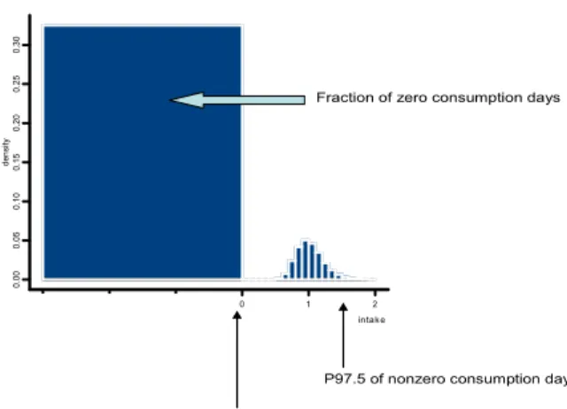
can only be solved by appropriately modeling the consumption patterns in the population (see chapter 3). Figure 1 visualizes the dilemma of observed nonzeros and observed zeros.

-3 -2 -1 0 1 2 0 .00 0. 05 0 .10 0. 15 0. 2 0 0. 25 0. 3 0 intak e de ns ity

P97.5 of nonzero consumption days

P97.5 of ‘total population’

Fraction of zero consumption days

Figure 1 ‘Consumers only’ (= nonzero consumption days) or ‘total population’?

Consumption days are depicted as a distribution of observed zeros and nonzeros. Since only few consumption days are sampled, there will be many zeros in the case of incidentally eaten foods. The effect of selecting the 97.5th percentile of ‘nonzeros’ (‘consumers only’) versus ‘total of nonzeros and zeros’ (‘total population’) is indicated, and illustrates a pragmatic dilemma. Note that for each food item the relative surface area of zeros and nonzeros will be different.

From the above it follows that when the interest lies in assessing the safety of actually eating a commodity, for pragmatic reasons it is preferable to use the ‘consumers only’ approach (in the first tier). When one is however interested in the probability that the ARfD is exceeded, one should take into account that the commodity is eaten incidentally or frequently, and therefore the total dataset, including the zero intakes, should be used. One should be aware that in the case of an infrequently eaten commodity, e.g. papaya, the latter approach may result in setting an MRL such that every time someone eats a papaya with a residue at the MRL he/she is at risk. However, since only a small percentage of the total population will eat papaya, this probabilistic approach may lead to the conclusion that the risk is acceptable. In this way acceptable risks are made comparable between more and less frequently consumed commodities. Yet, the situation of the papayas example is often referred to as ‘diluting the risk’, but this appears inappropriate terminology.

The above illustrates that is is very important to explicitly define which question is at stake, and which decisions on the procedure are taken.

(14)

2.5 Insights derived from probabilistic modeling

Probabilistic modeling offers the tool to combine knowledge about uncertainties and variability and abandons ‘piling up’ of worst case assumptions. Probabilistic modeling may be necessary when the margin between conservatively estimated exposure and conservatively estimated safe intake levels is small. As may become clear from the subsequent chapters a probabilistic risk assessment is more laborious than a deterministic risk assessment. Though probabilistic modeling itself is not too difficult because of available software, conceptual knowledge is needed to define how probabilistic modeling should be applied. Instead of having a point estimate, probabilistic modeling provides the risk assessor with distributions that can offer various insights.

The insights that can be derived from probabilistic chronic exposure assessments are: • The intake distribution of the whole population, and if required, from several

subpopulations for single foods and multiple foods.

• The percentage of the (sub)population exceeding an ADI, TDI for single foods and multiple foods.

The insights that can be derived from probabilistic acute exposure assessments are: • The probability that individuals may exceed an ARfD

• The percentage of the (sub)population having any certain probability of (not) exceeding the ARfD.

Unfortunately, a methodology for assessing the intake from multiple foods (see paragraph 2.7) is not yet available in the case of acute exposure.

Furthermore, the effect of intervening measures (for example recall of contaminated foods, long-term reduction of contamination) on the intake distribution of the (sub) population can be provided.

It may be clear that by providing intake distributions, policy management decisions on how to use these distributions should be taken. In the case of acute exposure assessment,

statements on which fraction (x) of the (sub)population may have a defined (y) probability of exceeding the ARfD are necessary.

2.6 Probabilistic approaches

Depending on the question at stake, the probabilistic approach required for providing useful answers may differ. In Chapter 4 we distinguish four domains of dietary exposure

assessment, each with its own difficulties. These domains are depicted in Table 1.

Table 1 Different domains of dietary exposure assessment.

Frequent intake Incidental intake

Long-term exposure A B

Acute exposure (single day) C D

A frequent intake implies a limited amount of observed zeros, whereas an incidental intake means a high amount of observed zeros. While with frequent intake zeros may be ignored without having much influence on the dietary intake distribution, with incidental intake one has to deal with these observed zeros. Furthermore, how to deal with the information ‘hidden’

(15)

in consumption data further depends on the question that is posed. Are we interested in the long-term exposure (to compare with ADI) or in the short-term exposure (compare with ARfD). Especially estimating the dietary risks of ‘acute exposure’ is a complex problem. Apart from variation in concentrations variation in consumption amounts as well as in consumption frequencies (intra-individual variation) has to be taken into account (for elaboration on this issue see following chapters).

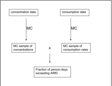
The probabilistic modeling approach proposed by Boon et al., (2004) from the RIKILT Institute focuses on the acute dietary intake (domains C, D) of the total population. It selects a consumption day randomly from the consumption dataset. The consumption rate of every single food item on that particular day is multiplied by a randomly selected residue concentration available for that food item. Then the calculated intake is divided by the individual’s body weight. This procedure is performed many times, resulting in a frequency distribution that reflects all plausible combinations of consumption and residue levels. The probabilistic approach proposed by RIKILT results in a distribution of person-days, but is often interpreted as a distribution of persons (which is incorrect). The outcome of the probabilistic approach proposed by RIKILT can be phrased as:

The probability that any person on any day exceeds the ARfD by eating one or more servings of a contaminated food item is Z%.

Though this outcome may seem useful, one should be aware that the probability of exceeding the ARfD on a single day might substantially differ between individuals. It might be that most individuals have a similar, but low probability of exceeding the ARfD, but it might also be that few individuals exceed the ARfD with a large frequency. Since the proposed approach cannot distinguish between both scenarios, it does not allow for a conclusion about the

fraction of the population at risk. Therefore, a decision based on the fraction of the population that should not exceed the ARfD (or, vice versa, a fraction for which it is accepted that the ARfD is exceeded), cannot be made. Although the proposed approach gives some insight in the distribution of daily intakes that may occur in humans, it still does not give the answer that would give a complete picture of the risks in the human situation. This answer should be formulated as:

x% of the population has a lower than y% probability to exceed the ARfD on any particular day

A probabilistic exposure model for acute dietary exposure that provides risk managers with such an outcome has been recently developed at RIVM (Slob and Bakker, 2004; Slob, 2005). The statistical model allows for estimating the distribution of consumption frequencies. Together with earlier developed models for estimating the distribution of (nonzero) amounts consumed, this results in a complete picture of the consumption patterns of single foods. This model can be combined with distributions of concentrations (e.g., by Monte Carlo sampling, where samples are taken from the model of intakes rather than from the observed intakes themselves).

2.7 How to deal with more foods?

A relevant risk management’s question is: ‘Is the exposure from multiple foods acceptable?’ This question has also been considered in the approach that is now in use for MRL-setting. The 1997 FAO/WHO Consultation already stated that ‘the consumption of two different

(16)

commodities in large portion weights by an individual consumer in a short period of time is not likely. Furthermore, the presence on those commodities of the same pesticide at the level of their MRLs is considered even less likely.’ (FAO/WHO, 1997)

When an MRL for a particular commodity is at stake while MRLs for the same pesticide are already established for other commodities, it may be argued that only the food item under consideration should be modeled at the level of field trial data. The remaining food items should be modeled at monitoring residue levels (‘background’ residue level).

A methodology to assess the exposure from multiple foods is only available for long-term exposure and frequently eaten foods (Slob, 1993). For both the long-term exposure and short-term exposure to incidentally consumed single foods a methodology has only recently

become available (Slob and Bakker, 2004; Slob, 2005). Unfortunately, a model that takes into account more than one food item has not yet been developed. For acute exposure the

construction of such a model is complicated since the correlation between the consumption of several food items should be taken into account. How to deal with correlations in a model for food consumption has not been worked out yet. Moreover, information on such correlations may be poorly available from data from the Food Consumption Surveys. Table 2 summarizes the availability of probabilistic approaches.

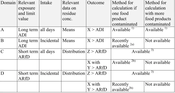
Table 2 Scheme of the various domains in dietary intake calculations with indications of their availability. Domain Relevant exposure and limit value Intake Relevant data on residue conc.

Outcome Method for calculation if one food product contaminated Method for calculation with more food products contaminated A Long term ADI

all days Means X > ADI Available 1) Available 1)

B Long term

ADI

Incidental Means X > ADI Recently available 2a)

Not available

C Short term

ARfD

all days Distribution Z > ARfD Available 3)

X with

Y > ARfD Available

2b) _{Not available}

D Short term

ARfD Incidental Distribution Z > ARfD Available

3) X with Y > ARfD Recently available2b) Not available X = fraction of the population; Y = frequency of exceeding the limit; Z = fraction of person-days.

1) _{e.g., STEM (Slob, 1993), Nusser (Nusser et al,1996)} 2a) _{STEM.II (Bakker and Slob, 2004; Slob, 2005)}

2b) _{STEM.II in combination with Monte Carlo from concentrations (Bakker and Slob, 2004;}

Slob, 2005)

3) _{MCRA (Boon et al., 2004)}

As long as such a tool for acute exposure assessment of for multiple foods is not available a more pragmatic approach may be followed. The MCRA methodology suggested by Boon et

al., (2004) (RIKILT) considers recorded days as such. A person-day of the food consumption

(17)

combined with a randomly drawn concentration of each food, using a Monte Carlo approach. The total pesticide intake (corrected for the person’s bodyweight) is calculated. By repeating this procedure many times an intake distribution is obtained. Since the MCRA methodology considers recorded days as such, one should be aware that the results are difficult to interpret since the distribution does not reflect individuals, but person-days. However, as long as no other tool is available, the distribution obtained by MCRA may be used as an indication of plausible daily intakes when the pesticide could occur on various foods.

The CCPR 36 Working Group performed several calculations with the MCRA approach using supervised field trial data for all commodities. It was observed that in some cases there are significant contributions from more than one food item in the upper part of the

distribution of person-days, e.g. when the residue has been measured in commonly eaten foods like wheat, potatoes, rice. However, generally the Working Group concluded that ‘high exposures resulting from multiple high commodity exposures occur seldom, usually the contribution from one commodity dominates the outcome’.

2.8 How to deal with cumulative and aggregate exposure?

An area under development is the assessment of cumulative and aggregate exposure to

chemicals. ‘Cumulative exposure’ refers to different chemicals with the same mode of action, while ‘aggregate exposure’ refers to exposure to a chemical from different sources, e.g. a chemical that is used as a pesticide (exposure through food), but which also is included in shampoo (exposure through skin). When one is interested in cumulative exposure of ‘similar acting chemicals’, an additional assumption is needed, viz. that of dose additivity. This assumption is not so easy to validate, as it requires quite complicated studies involving the exposure to various mixtures of various numbers of compounds. In addition, relative potency factors (TEFs) can usually only be estimated from studies on single compounds, which have often used sub-optimal study designs (e.g. few, or not optimally placed doses). This will result in uncertainties in the estimated TEFs. However, these uncertainties should be

quantifiable (when they are assessed by the Benchmark approach), and can thus be taken into account (Crump, 1984; Slob and Pieters, 1998). Note that cumulative exposure assessments for acute and chronic exposure, should be based on acute and chronic TEFs, respectively. For a more detailed review of cumulative exposure assessment of acetylcholine-esterase

inhibitors, see van Raaij et al., (2004). It may be noted that assessments for cumulative and aggregate exposure can only be done on a total population basis.

2.9 Health risk at actual exposure levels

The question whether an MRL is safe by itself is different from the question whether there is a risk in a realistic situation of actual pesticide use. In real life situations, the residue

concentrations of consumer-ready products will be below the MRL in many cases. When the MRL is exceeded the question arises if there is a health risk associated with this exceedence. ‘Real life’ monitoring data are far more relevant than the data from supervised trials in assessing health risks in an existing situation. Note that these data may reflect a ‘worst case’ situation when the sampling has not been performed at random, but directed to lots suspected from high contamination. The distribution of consumption in the population will give more insight in the dietary intake than a chosen (high) percentile of this distribution.

(18)

Consumption advises

Yet another question that may be posed is if particular (extreme) consumption behaviours may result in health risks. The influence of consumption behaviour on the intake, i.e., what is the effect of eating one, two, three contaminated apples can be easily calculated. If it turns out that (extreme) consumption of a food may be associated with a health risk, this insight may lead to food consumption advises in those cases that occurrence of a substance on a food cannot be avoided.

(19)

3. Probabilistic modeling: a short introduction

3.1 The need for probabilistic modeling in risk assessment

The risk assessment of substances comprises exposure assessment and effect assessment. Human limit values such as ADI, TDI, ARfD are the result of an effect assessment (hazard characterisation) and are considered to be ‘safe’ for the total population. These limit values are based on toxicological data and considerations. They are generally derived by using worst

case assumptions regarding potential differences between experimental animals and humans,

as well as regarding the variability in sensitivity within the human population. Next, product limits may be derived, based on these health-based human limit values, in combination with information on human behaviour relevant for exposure (e.g., consumption rates for foods) Product limits such as maximum residue limits (MRLs) for pesticides are set based on other considerations: the application of a substance on commodities using Good Agricultural Practice (GAP) in supervised trials. MRLs are based on residue concentrations measured after observing a defined preharvest interval following the application of the pesticide. Next, it is determined whether or not food items with pesticides present at concentrations at the MRL may result in human intakes to exceed the ADI or ARfD. In these calculations, the intake is currently based on worst case assumptions concerning the consumption rate of the commodity.

Both the exposure and effect assessment approaches just mentioned may be considered as conservative, and as such may suffice for situations where the margin between the estimated exposure and the human limit values is large. Here we are in the ‘no problem’ zone and a more adequate assessment will not be necessary. However, when the margin between estimated exposure and estimated safe intake levels is smaller a more precise estimation of both intake and of ‘safe‘ doses may be required. Probabilistic modeling offers the tool to combine knowledge about uncertainties and variability and abandons ‘piling up’ of worst case assumptions.

For the derivation of human limit values probabilistic methods offer the possibility to derive probabilistic limit values without being overly conservative (protective), see e.g. Slob and Pieters (1998). Similarly, probabilistic exposure modeling offers the possibility to arrive at a complete description of the exposure in the human population taking the variation between individuals and in food levels into account. Next, in a probabilistic risk assessment, one may follow two routes. One is to compare the (probabilistic) limit value with the probabilistic exposure estimate. The other is to estimate the possible health effects in (a specific part of) the human population at a given level of exposure, again in a probabilistic way. The risk assessment carried out for the mycotoxin deoxynivalenol (DON) is an example of this methodology (Pieters et al., 2004).

When a more precise risk assessment is needed risk assessment assumptions made in exposure and effect assessment are often looked upon in more detail and may be adjusted from ‘default’ values to more substance or commodity specific assumptions. Probabilistic modeling offers the tool to combine knowledge about uncertainties and variability concerning all the subparts of the assessment, resulting in a probabilistic statement on the expected health effect in a certain fraction of the population. In this report we focus on probabilistic modeling of dietary intake.

(20)

3.2 What is probabilistic modeling?

Probabilistic modeling refers to combining distributions of variables, instead of using worst-case deterministic (or point) values for these variables. Probability or frequency distributions describe the range of values that variables may take, together with the probability (frequency) that the variable will take any specific value.

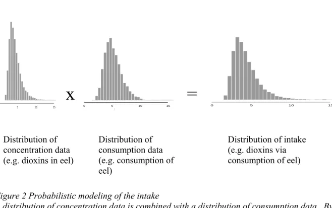
For example, instead of multiplying the average dioxin concentration measured in eel by the average consumption of eel, a distribution of the concentration data is combined with the distribution of consumption data. By performing (Monte Carlo) sampling from the two distributions, multiply the two sampled numbers, and repeat this many times (iterations) the outcome may also be presented as a distribution (Figure 2). This Monte Carlo approach can be applied very generally, whatever the type of calculation, or whatever the distributions applied. The answer has some element of noise in it, and one needs to make sure if a sufficient number of iterations was used. In some situations, the resulting distribution can also be derived from simple calculations (Slob, 1994).

Figure 2 Probabilistic modeling of the intake

A distribution of concentration data is combined with a distribution of consumption data. By performing many iterations the resulting intake may also be presented as a distribution.

Carrying out probabilistic modeling by Monte Carlo methods is not difficult. There are various commercial software packages on the market (e.g., Crystall Ball, @RISK) that reduce the computational effort of doing the random sampling.

The advantages of probabilistic modeling in risk assessment are that uncertainties can be quantified and that variability in the population is taken into account. Furthermore, the main sources of uncertainty can be identified, and may subsequently be subject for further

measurements or study. 0 5 10 15 EF intra 0 5 10 15 EF inter 0 5 10 15 EF intra

=

x

Distribution of concentration data (e.g. dioxins in eel)

Distribution of consumption data (e.g. consumption of eel)

Distribution of intake (e.g. dioxins via consumption of eel)

(21)

The important issue is how to use probabilistic modeling (which variables are relevant to the question) and how to interpret the final result. For this, some understanding about the

differences between variability and uncertainty is necessary.

3.3 Variability and uncertainty

Variability refers to the range of values that really occur within the system considered.

Variation within a (human) population is ubiquitous, e.g. concerning height, hair color, food consumption. Each unit in the system (or each individual in the population) may have a different value. Variability cannot be reduced by further measurements. By quantifying variability a statement is made about the fraction of the population (e.g., eating fish at least once a week).

Variability usually has different levels. For example, daily consumption rates may vary between persons, vary between consecutive days, vary between seasons, vary between days of the week, vary between countries, etc. Which levels of variability are relevant is

determined by the question at stake. When different characteristics of the same units are considered, it may be necessary to take correlations into account. For instance, body weights may be correlated to consumption behavior

Uncertainty refers to the limited knowledge or imprecision in the estimate concerning a

(single) value, e.g. the average consumption of eel, the mean residue concentration on a crop, the Kow of a compound. As a more complicated example, there may be uncertainty regarding variability. For instance, the variation in consumption rates of potatoes may be somewhere between a coefficient of variation (CV) of 18% and 24% (i.e., a range expressing the uncertainty in the CV). Further studies or measurements can reduce the uncertainty

associated with this particular value. By quantifying uncertainties a statement is made about the probability of being wrong. A typical way of expressing uncertainty is by a confidence interval, which is interpreted as an interval containing the true value (by some level of confidence).

In probabilistic modeling practice the distinction between uncertainty and variability is not always maintained. It is however paramount to separate uncertainty from variability in any particular assessment, otherwise the finally resulting distribution cannot be interpreted.

(22)

4. Probabilistic modeling of intake of substances via

food: the question determines how to proceed

4.1 Consumption frequency

To gain insight in the consumption behavior national food consumption surveys have been performed. The Dutch Food Consumption Survey describes the consumption over two consecutive days from 6250 individuals belonging to 2564 households (Kistemaker et al., 1998). Depending on the food item of interest the number of observed consumption days (i.e. days with a nonzero observed consumption of a particular food) will vary. The maximum number of consumption days in this survey is 12,500. However, for many foods the number of observed consumption days will be lower since most food items are not consumed daily. The consumption frequency is defined as the probability that an individual consumes the food item on a single day. The consumption frequency differs among individuals. Some will consume a certain food item regularly, others incidentally and some people will ‘never’ consume the food item. The observed days with zero consumption are sometimes referred to by the term ‘non-consumers’. This is improper, and the term zero-consumption day is preferable to avoid misunderstanding. Note that an observed zero consumption on two (or more) days does not imply that the pertinent individual is a non-consumer. With increasing numbers of sampling days in a year, the probability increases that an individual will have some nonzero consumption days even when they do not like the food. In other words,

individuals classified as non-consumer in a two-day food consumption survey may turn out to be classified as consumer in a survey with longer study duration. The latter was nicely

illustrated by Lambe et al., (2000), based on real consumption data.

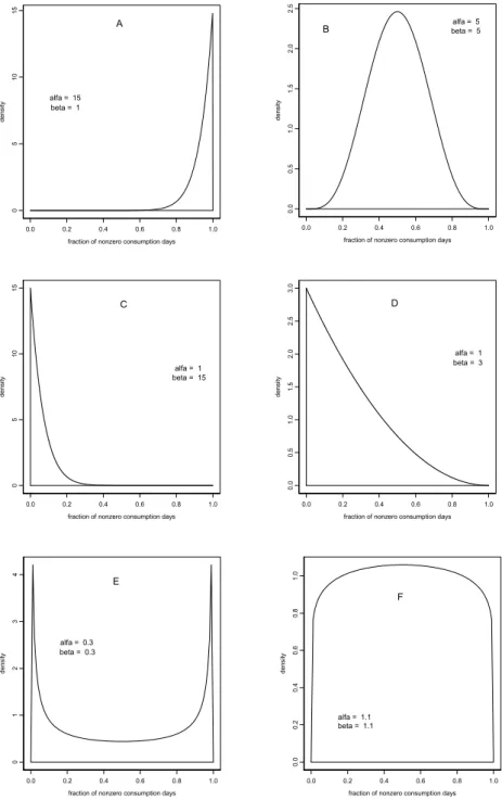
In the case of food items that are consumed by almost everyone on almost all days (such as bread) the consumption frequency may be shaped as depicted in Figure 3A. The area under the curve represents 100% of the population. When the fraction of consumption days is low (e.g. 10%), the corresponding area under the curve is also low, indicating that only a small part of the population will consume the product in less than 10% of the days. A large fraction of the population consumes the product in more on than 90% of the days.

In the case of food items that are more or less regularly consumed by most people (such as eggs or egg-products), the consumption frequency may be shaped as depicted in Figure 3B. Here only a small fraction of the population will consume the product in less than 10% of the days, or in more than 90% of the days.

Another extreme scenario is that the food item is consumed incidentally by almost everyone, for example spice nuts (‘pepernoten’) which are mainly consumed in the period around a Dutch yearly festivity. This kind of scenario is reflected by Figure 3C (for spice nuts the distribution may even be more extremely squeezed to the left). As another example, Figure 3D reflects the situation where many people consume the food item incidentally (for example in less than 10% consumption days) while fewer people consume the product more regularly. This distribution thus shows a larger variation between people than Figure 3C.

In the scenario reflected by Figure 3E a large part of the population consumes the product quite regularly, while a small fraction of the population tends to avoid it, and another small fraction tends to consume it very frequently. Figure 3F also shows a scenario where all

(23)

consumption frequencies are more or less equally likely, but with few avoiders or frequent consumers.

0.0 0.2 0.4 0.6 0.8 1.0

fraction of nonzero consumption days

0 5 10 15 densit y alfa = 15 beta = 1 A 0.0 0.2 0.4 0.6 0.8 1.0

0. 0 0. 5 1. 0 1. 5 2. 0 2. 5 densit y alfa = 5 beta = 5 B 0.0 0.2 0.4 0.6 0.8 1.0

0 5 10 15 densit y alfa = 1 beta = 15 C 0.0 0.2 0.4 0.6 0.8 1.0

0. 0 0. 5 1. 0 1. 5 2. 0 2. 5 3. 0 densit y alfa = 1 beta = 3 D 0.0 0.2 0.4 0.6 0.8 1.0

0 123 4 densit y alfa = 0.3 beta = 0.3 E 0.0 0.2 0.4 0.6 0.8 1.0

0. 0 0. 2 0. 4 0. 6 0. 8 1. 0 densit y alfa = 1.1 beta = 1.1 F

Figure 3 Illustration of different consumption frequencies in the population 3A. Consumption by almost everyone on almost all days (e.g. bread). 3B. Regular consumption by most people (e.g. eggs). 3C. Incidental consumption by almost everyone (e.g. spice nuts). 3D. Incidental consumption by many people, fewer people have consumption on a more regular basis. More variability compared to 3C. 3E.: avoidance of consumption by a large group while another large group favors the food item (e.g. salted herring). 3F: consumption frequencies are equally likely.

(24)

Since in the Dutch Food Consumption Survey only two days per individual were registered, the data do not seem to provide the information to estimate the distribution of consumption frequencies. Yet, it could be shown by computer simulations (Slob and Bakker, 2004) that the frequency distribution can reasonably be estimated for data as provided by the Dutch Food Consumption Survey, i.e., only two days per individual, but for a large number of individuals. Similar results were obtained for data with less individuals but more days per individual.

4.2 Domains of risk assessment queries

In chapter 2 we presented different risk management questions. Risk managers may be interested in the safety of a product limit (such as MRL), in the health risks associated with the consumption of a contaminated lot exceeding an MRL or in the health risks at actually measured residue concentrations. In the case of a long-term exposure the estimated intake should be compared to human limit values assessed for chronic exposure (ADI, TDI, RfD). In the case of a single-day exposure the estimated intake should be compared with a human limit value assessed for such a short-term exposure, such as an Acute Reference Dose (ARfD).

In the case of general food items such as bread, milk products, which are consumed (almost) every day by (almost) 100% of the population, the number of consumption days is large. The consumption is referred to as ‘frequent’. When the food item is consumed incidentally, the number of ‘zero’ consumption days will be larger. As illustrated in Figure 3 the occurrence of ‘zero’ consumption days can be explained by different consumption scenarios.

However, our interest is not the consumption of a food item, but the intake of a chemical. Various food items may contribute to the total dietary intake, for example a pesticide used on various fruits and vegetables. Though the consumption of a certain fruit may be considered as incidental consumption, the intake of the chemical may occur on almost all days and in all individuals.

The domains of risk assessment queries may be presented in a 2 by 2 matrix (Table 1). For each of these four domains of risk assessment another type of information and model is needed. Though the Dutch Food Consumption Survey is a large sample of the Dutch

population, the information in the available data is still limited in various respects. Depending on the risk assessment query the approach of how to use and interpret the data may be

different.

Table 1 Different domains of risk assessment queries.

Frequent intake Incidental intake

Long-term exposure A B

Acute exposure (single day) C D

In domain A one is interested in possible health effects due to a long-term frequent intake of a chemical. If sufficient concentration data are available the exposure assessment can be performed relatively well. The exposure assessment of ochratoxin A (Bakker and Pieters, 2002), fumonisin B1 (Bakker et al., 2003), DON (Pieters et al., 2004) and dioxins and PCBs

(25)

Recently, an approach for how to deal with long-term incidental intake (domain B, for example red wine) has been developed (Slob and Bakker, 2004). How to deal with acute (single day) exposure (C and D) is a more difficult issue as will be explained later. As an example, one may be interested in the acute risk of the consumption of mangos with a high level of residue (D) or in a temporarily high contamination of a staple food (C).

4.3 Domain A. Long-term exposure, frequent intake

The variation in the observed daily intakes has two components: a within-subject and

between-subject variation. Since in domain A one is interested in the long-term exposure, the between-subject variation is a relevant level of variation, whereas variation between days (the within-subject variation) is not. However, the observed distribution of consumption data includes both levels of variation. With statistical modeling it is possible to estimate the between-subject variation by correcting the observed total variation for the daily variation within subjects. For this purpose RIVM developed the Statistical Exposure Model STEM (Slob, 1993; Slob, 1994), but also other (similar) models are available (Nusser et al.,1996). STEM estimates the median dietary intake as a function of age. By using these models and the average concentration of the chemical in each food item the inter-individual variation in the long-term exposure can be estimated. Since we are interested in long-term exposure the use of distributions of concentrations has not much added value. Note that this is approach is a probabilistic assessment without using Monte Carlo methods.

The results of these calculations may be expressed in various ways:

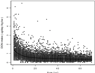
I. The estimated intake (median and percentiles) as a function of age (see Figure 4)

0 2 0 4 0 6 0 A ge (y r ) 01 23 4 5 6 D O N i nt ak e ( ug/ da y / kg bw )

Figure 4 Daily intake as a function of age. Each dot denotes one daily intake of a single individual. The uninterrupted curve represents the estimated median intake assessed by fitting a regression function to all points. The dashed curves denote the 95th and 99th percentiles, indicating the long-term variation between individuals. (from: Pieters et al., 2002). Note that the variation in the dots is larger than that indicated by the percentiles, as the percentiles only represent the variation between subjects, and not within subjects.

(26)

II. For each age-class the intake distribution can be deduced from the median intake and the estimated between-subject variation. See Figure 5, for an example.

0 0.1 0.2 0.3 0.4 0.5 0.6 0.7 0.8 0.9 1 0.0 1.0 2.0 3.0 4.0 5.0

DON intake µg/kg bw/day

Pr

ob

ab

ili

ty density

Figure 5 Distribution of DON intake at age 2 (from: Pieters et al., 2002).

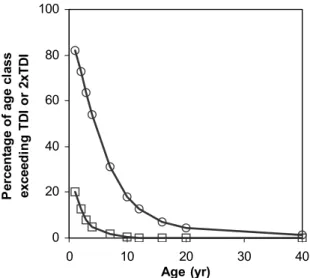
III. Fraction of population exceeding the human limit value (TDI, ADI), as a function of age. For example, see Fig.6.

0 20 40 60 80 100 0 10 20 30 40 Age (yr) P er cen ta g e o f ag e cl as s exceed in g T D I o r 2xT D I

Figure 6 Percentage of age-classes exceeding the TDI (circles) or twice the TDI (squares). (from: Pieters et al., 2002).

In the case of frequent intake and long-term exposure, it is thus possible to assess the intake in relation to age and to calculate the fraction of the population as a function of age that exceeds the TDI. It should be noted that various assumptions were needed here. For instance, the within-subject variation can be estimated from the data on all subjects by assuming that the within-subject variation is homogeneous for different persons. This may not be perfectly true, but the final result may be relatively insensitive for moderate violations of this

(27)

4.4 Domain B. Long-term exposure, incidental intake

Since the long-term exposure is of interest, the between-subject variation is relevant (as in domain A), whereas the within-subject variation is not. The difficulty in this domain is caused by the fact that for incidentally consumed food items the recorded consumption days will comprise many observed zeros, as depicted in Figure 2. The terms ‘consumer’ and ‘non-consumer’ to indicate the difference between observed zeros and observed nonzeros are misleading. What is observed are person-days and not ‘real’ persons. One person may have been a consumer at day one (nonzero observation), and a non-consumer at day 2 (zero observation). Or, a person recording a zero on both days may be a consumer for the rest of the year (and vice versa). Thus, it seems impossible to obtain information on how individuals vary with respect to consumption frequency when only two recorded days per individual are available. Yet, we showed (by computer simulations, see Slob and Bakker (2004) that this is possible, when it is assumed that the consumption frequency can be adequately described by a so-called Beta distribution. The complete data set from the Food Consumption Survey is used to estimate this distribution for consumption frequency. The Beta distribution has only two parameters and is defined between 0 and 1 (or 0 and 100%). The advantage of the Beta-distribution is its flexibility (as illustrated in Figure 2), so that it can adjust to many forms and is therefore suitable for describing many (theoretical) consumption frequencies.

This approach has been incorporated in a recently developed model, called STEM.II, which describes the consumption of incidentally consumed products in the total populations (Slob and Bakker, 2004). Since it is likely that the consumption frequency of food items generally depends on age, the Beta distribution may be different for different ages. The number of observed consumption data for single age classes would, however, not suffice to estimate the Beta distribution for each age class separately. Therefore, it is assumed in STEM.II that one of the parameters of the beta-distribution may depend on age, while the other does not. In this way, the mean of the distribution may change with age, and this relationship may be

described by a regression function. For an illustration of this method, see Figure 7.

In addition, the amount of the intake (on a consumption day) may depend on age as well. Just as in domain A, the total variation of observed intakes should be corrected for the within-subject variation (e.g. Slob 1993; Nusser et al., 1996), since only the between-within-subject variation is relevant for long-term exposure.

Finally, the (age-dependent) distributions of intake frequencies and the (age-dependent) distributions of intake amounts are combined to calculate:

The fraction of individuals with an average intake that exceeds the ADI, as a function of age

(28)

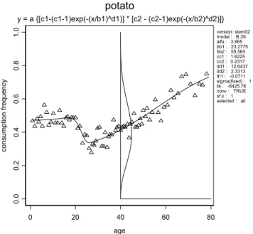
Figure 7 Relation between consumption frequency and age described by a nonmonote model (fitted curve). De triangles show the mean observed frequencies per age class by grouping all individuals in the age class together. For the age class 40 the Beta-distribution is drawn, showing the variation in consumer frequency for 40-years old people. In total 8 parameters are estimated from the data in this case.

Although Figure 7 may appear complex, the results of this approach can also be presented in ways providing immediate insight towards policy queries. Suppose that the limit value for red wine is 100 ml. In Figure 8 the fraction of the population with a long-term consumption of wine higher than 100 ml/day is plotted as a function of age. As expected, in children this fraction is very low. Further, it can be seen that the fraction decreases at higher ages.

Figure 8 Fraction of the population with a long-term intake above 100 ml of red wine, as a function of age. 0 20 40 60 80 age 0.0 0. 2 0.4 0. 6 0. 8 1.0 consumpt ion f reque ncy potato version: stem02 model : B 29 alfa : 3.865 bb1 : 23.2775 bb2 : 55.565 cc1 : 1.6225 cc2 : 0.2317 dd1 : 12.6437 dd2 : 2.3313 th1 : -0.0711 sigma(fixed) : 1 lik : -6425.78 conv : TRUE sf.x : 1 selected : all y = a {[c1-(c1-1)exp(-(x/b1)^d1)] * [c2 - (c2-1)exp(-(x/b2)^d2)]} 0 20 40 60 80 age 0.000 0 .005 0. 010 0. 015 0.02 0 0.025 0 .030 fr act ion of popul ati on