small-scale monopile scour protection experiments
Data analysis of the 3D damage number in
Academic year 2019-2020
Master of Science in Civil Engineering
Master's dissertation submitted in order to obtain the academic degree of
Counsellors: Minghao Wu, Carlos Arboleda Chavez
Supervisors: Prof. dr. ir. Peter Troch, Dr. ir. Vicky Stratigaki
Student numbers: 01505499, 01404669small-scale monopile scour protection experiments
Data analysis of the 3D damage number in
Academic year 2019-2020
Master of Science in Civil Engineering
Master's dissertation submitted in order to obtain the academic degree of
Counsellors: Minghao Wu, Carlos Arboleda Chavez
Supervisors: Prof. dr. ir. Peter Troch, Dr. ir. Vicky Stratigaki
Student numbers: 01505499, 01404669i
Preamble
The main objective of this research was initially to perform experiments in the large wave flume in the Coastal Engineering Research Group (CERG) of Ghent University, on the stability of scour protection around a monopile of a wind turbine, under the combined action of waves and currents. The study would have been done by repeating selected tests from the experimental test programme accomplished during the PROTEUS project, at a smaller scale, to investigate potential scale effects.
Due to coronavirus measures imposed by Ghent University, laboratory work for thesis students was not allowed, so the experiments in the wave flume foreseen for March-April 2020, did not go through as planned, leading to a reorientation of the thesis in March.
As a lot of time had already been invested in literature research and setting up the experiments, this is still a considerable part of this thesis. Both a literature study on scour and scale effects and a chapter on the set-up of the experiments are included. This work will be valuable for the future, when the tests will be allowed. The actual research of this thesis shifted from carrying out our own small-scale experiments to a desk study with re-analysis of an existing dataset from 2008 on scour protection damage, using a newly implemented correction of the monopile offset and a new script, as well as a detailed study on the FARO® Freestyle3D handheld laser scanner for measuring scour damage in a small scale model set-up.
This preamble was written in consultation between the students and the promotors and is agreed upon by both parties.
Deze pagina is niet beschikbaar omdat ze persoonsgegevens bevat.
Universiteitsbibliotheek Gent, 2021.
This page is not available because it contains personal information.
Ghent University, Library, 2021.
iii
Summary
Title: Data analysis of the 3D damage number in small-scale monopile scour protection experiments
Authors: Ramon Debaveye, Bram De Riemacker Promotors: Prof. dr. ir. Peter Troch, dr. ir. Vicky Stratigaki Counsellors: Minghao Wu, Carlos Arboleda Chavez
Master’s dissertation submitted in order to obtain the academic degree of Master of Science in Civil Engineering
Faculty of Engineering and Architecture Department of Civil Engineering
Academic year 2019-2020
Keywords: Monopile foundation, scour protection, small-scale experiments, scale effects, 3D damage number, FARO® Freestyle3D handheld laser scanner, EPro
Abstract
The initial goal of this paper was to conduct experimental research on scale effects in the physical modelling of the scour protection of monopiles. The small-scale tests would have been performed in the wave flume at Ghent University and are a follow-up of the PROTEUS project. One of the goals of the PROTEUS project was to provide a high quality benchmark dataset for future experiments. The eroded profiles would have been measured with the FARO® Freestyle3D handheld laser scanner.
In the first part of the thesis, a literature study is done on the subjects of scour and scale effects in physical modelling. This knowledge allows the experimenters to gain the necessary insight before attempting to do small scale physical model scour protection tests themselves.
In the second part, a test set-up for the experiments is proposed. The parameters from the PROTEUS project have been downscaled to the large wave flume available at the Department of Civil Engineering. In the third part, a step-by-step guide on how to use the FARO® Freestyle3D handheld laser scanner is included, in order to allow future users to easily familiarize themselves with the device.
The planned tests have been cancelled and the research conducted in this paper has shifted to a data re-analysis of the tests performed in De Vos (2008). The objective of this work is to validate a new damage calculation script which is used to calculate the three-dimensional damage number for scans performed with the FARO® Freestyle3D handheld laser scanner. This is achieved by analysing the raw data obtained during the tests of De Vos (2008) and comparing the damage calculation of the EPro software to the damage calculation of the new script. Additionally, an objective comparison is made between the two methods. It appeared that the script works as intended, as its results do not differ much from the results obtained with EPro. Minor differences can be attributed to a difference in the integration method and subzone division method. The integration method for the handheld laser scanner script could be refined more in the future. It was furthermore found that the handheld laser scanner can produce results with the same or higher accuracy as EPro. Its accuracy can even be lower than 1 mm. Both devices have their own (dis)advantages, depending on the scale and type of experiments.
Data analysis of the 3D damage number in
small-scale monopile scour protection experiments
Ramon Debaveye, Bram De Riemacker
Supervisors: Prof. dr. ir. Peter Troch, dr. ir. Vicky Stratigaki, Minghao Wu, Carlos Arboleda Chavez
Abstract: The initial goal of this thesis was to conduct experimental research on scale effects in the physical modelling of the scour protection of monopiles in a combined wave and current climate. The small-scale tests would have been performed in the wave flume at Ghent University and are a follow-up of the PROTEUS project. One of the goals of the PROTEUS project was to provide a high quality benchmark dataset for future experiments. This dataset would have been scaled down and the eroded profiles would have been measured with a new erosion profiler which is a handheld laser scanner.
The planned tests have been cancelled and the research conducted in this paper has shifted to a data analysis of the tests performed in the PhD thesis of De Vos [1]. The objective of this thesis is to validate the applicability of the FARO® Freestyle3D
handheld laser scanner [2] in small-scale monopile scour protection experiments. This is achieved by analysing the raw data obtained during the tests of De Vos [1] and comparing the damage calculation of the EPro [3] software to the damage calculation using the handheld laser scanner. Lastly, an objective comparison is made between the two methods. This can be used as a guide to decide which method to use in future experiments in the wave flume.
Keywords: Monopile foundation, scour protection, small-scale
experiments, scale effects, 3D damage number, FARO®
Freestyle3D handheld laser scanner, EPro
I. INTRODUCTION
Renewable energy dramatically gained importance in the last few decades as the topic of climate change has become ubiquitous in the political and industrial agendas. Offshore wind farms make part of this renewable energy and form an attractive energy source due to their increased energy conversion efficiency compared to their onshore variants. However, the installation of offshore wind farms also comes with many challenges. One of those challenges is the high cost. Monopiles make up for 70% of the substructure and foundation choice for new offshore wind farms [4]. The cost of the foundation of a monopile is estimated to be 20% of the total cost [5]. An important engineering challenge in this process is the design of an economic and sustainable scour protection. The latter is needed to ensure the stability of the monopile under the combined effect of waves and current whilst taking into account cost and durability.
The PROTEUS project plays an important role in this development. Besides optimising the design of scour protection around offshore wind turbine monopiles and future-proofing them against the impacts of climate change, the main research goal of the experiments is to provide a high-quality benchmark dataset. This dataset can then be used as a basis for future tests.
An important part in the physical modelling process of scour protection experiments is accurately measuring the damage caused by the combined effect of waves and current. The damage is often represented by a dimensionless variant of the volume that has eroded away. An accurate measurement of the eroded volume is thus indispensable.
As the scale of the physical model becomes smaller, the accuracy of the required equipment has to follow the same trend. Until now, the erosion profiler (EPro) developed by the university of Aalborg has been used in the wave flume of the department of Civil Engineering at Ghent University. This profiler is commercially available as the volume measurement and damage calculation have been validated and its quality has been accepted. However, EPro also has some disadvantages of which its limited scanning speed and achievable accuracy are the most important ones. This has led to the introduction of a new erosion profiler at the Department of Civil Engineering at Ghent University: the FARO® Freestyle3D handheld laser scanner. The handheld laser scanner has been developed to produce high-quality scans of objects. The result of such a scan is a point cloud. Similar as in EPro, the obtained scan has to undergo a few post-processing steps in order to obtain the eroded volume and thus the damage number. In this thesis, the corresponding post-processing procedure is validated.
In this regard, a data analysis of real experimental data from the PhD thesis of De Vos [1] is required to be able to compare the damage calculation of the two methods. Firstly, a dry condition accuracy and sensitivity analysis of the handheld laser scanner is performed. Thereafter, a sensitivity analysis of the raw EPro data is executed, followed by a damage number comparison between the two methods. The latter plays an important role in the validation of the post-processing script. Finally, a summarising and objective comparison between the two methodologies is given.
II. WAVE FLUME SET-UP
A significant portion of the time was spent in the preparation of the wave flume set-up. Therefore, it is still included in the thesis as it has led to insight in conducting experimental research.
A. General description of the wave flume set-up
The wave flume of the Department of Civil Engineering at Ghent University is 1 m wide, 1.2 m high and 30 m long. A part of the concrete wall of the wave flume is replaced with glass panes supported on a steel frame to allow for visual observations during the tests.
The set-up of the small-scale monopile model consists of a sandbox construction, the wave absorption system, the measuring equipment, the wave generator and the current system.
The sandbox is 3.5 m long and to contain the monopile foundation with a transition piece for a pile of 10 cm in diameter.
The wave absorption consists of a passive wave absorption system and an active wave absorption system. The former consists of Hexablocks, for which a reflection coefficient of less than 30% is achieved [6]. The Hexablocks are placed at the opposing end of the wave generator. The active wave absorption system is part of the wave generation system. Wave reflection is measured and the movement of the wave paddle is adjusted accordingly.
The measuring equipment consists of six wave gauges and two velocimeters. They are required to check that the measured hydraulic conditions do not significantly differ from the target conditions.
B. Hydraulic test conditions
The hydraulic test conditions are directly derived from the PROTEUS tests [7]. They are scaled down according to Froude scaling, which is a consequence of the ‘Best Model’ described by Hughes [8]. A selection of the tests executed in the PROTEUS project had to be made since the available time in the wave flume is limited. The emphasis of the test program is put on quality and repeatability.
The generated waves are irregular waves with a JONSWAP spectrum with a peak enhancement factor γ of 3.3, which represents the conditions in the North Sea. The current is generated by an external pump circuit. However, the magnitude of the generated current is limited which, in turn, limits the number of executable tests.
In a wave flume, waves will interact with the current. For waves opposing a current, the wave height increases and vice versa. This effect has been quantified in the research conducted by Draycott et al. [9] and is formulated by equation (1).
𝐻
1= 𝐻
0√(
𝐶
𝑔,0𝐶
𝑔𝑟,1+ 𝑈
) ⋅ (
1
1 +
𝐶
𝑈
𝑔𝑟,1)
(1)
In equation (1), 𝐻1 is the wave height after wave-current
interaction and 𝐻0 is the base wave height. This effect has been
accounted for in the determination of the hydraulic conditions. The target wave height in the wave flume is the wave height after interaction, therefore, the input wave height for the wave generation software is 𝐻0.
C. Scour protection characteristics
The scour protection used in the small-scale experiments is obtained by geometrically scaling down the rock gradings used in the PROTEUS project. Due to the limited amount of available sieves, interpolation of the original PROTEUS sieving curves is necessary. Furthermore, to limit the amount of sieving work, three sieve sizes are used. This is possible since the available stones were already pre-sieved between 1 mm and 5 mm.
Figure 1 shows the downscaled sieving curves of tests 10, 12 and 13 of the PROTEUS project and the approximated sieving
curve obtained by using the available sieves and stones. The latter is the proposed grading.
Figure 1: Sieving curves of downscaled PROTEUS tests 10, 12 and 13 and their approximation with available sieves and stones.
Even though the number of sieves is limited, the downscaled rock gradings are approximated quite well.
D. Data analysis
During the execution of a test, it is required to check whether the measured conditions are sufficiently close to the target conditions. The data obtained from a test consists of the measured wave heights, the current velocity and the eroded profiles. The measured wave heights are analysed in Wavelab and are represented by a significant wave height. In order to calculate the damage, three scans are performed. One scan is taken before any hydraulic loads, a second one is taken after 1000 waves and finally a third scan is taken after 3000 waves. These scans are compared during post-processing. Additionally, a camera is mounted above the pile to capture the profiles.
The damage definition used in this thesis is in accordance with the work of De Vos [1]. The three dimensional damage number S3D is, in case of small-scale tests, defined as:
𝑆
3𝐷= max(𝑆
3𝐷,𝑠𝑢𝑏)
(2)
In equation (2), 𝑆3𝐷,𝑠𝑢𝑏 is the damage defined in a subzone.
The latter is defined as:
𝑆
3𝐷,𝑠𝑢𝑏=
𝑉
𝑒𝐷
𝑛50𝜋
𝐷²
4
(3)
In which 𝑉𝑒 is the eroded volume, derived from the eroded
profiles, 𝐷𝑛50 is the nominal median grain size of the scour
protection and 𝐷 is the pile diameter. The scour protection is divided into 24 sub areas just like in the work of De Vos [1] since it facilitates the data analysis. This is shown in Figure 2.
0 10 20 30 40 50 60 70 80 90 100 0 2 4 6 8 Pa ss in g ra te [ % ] Sieve size [mm]
Scaled Test 12 & 13 Scaled Test 10 Proposed grading
Figure 2. Sketch of the scour protection model around the monopile [7]
III. THE USE OF A HANDHELD LASER SCANNER IN SMALL -SCALE SCOUR EXPERIMENTS
The handheld laser scanner has not yet been used for measuring eroded profiles in small-scale experiments at Ghent University. As such, there is no extensive knowledge and experience with the device for this purpose. An important process during this thesis is getting familiar with the device and developing a methodology to produce high quality scans. In this regard, a step-by-step guide has been developed which can be used by future users. The guide describes the required steps needed to physically execute a high quality scan up to the point where processable data is available.
The guide starts with a description of the device. Thereafter, the physical execution of a scan is discussed. This is followed by a description of the post-processing procedure with emphasis on how to align scans taken before and after hydraulic loads. The alignment of the scans plays an important role in the achieved precision of the handheld laser scanner and thus of the reliability of the obtained damage number.
IV. VALIDATION OF THE HANDHELD LASER SCANNER DAMAGE CALCULATION
The new post-processing methodology is validated by comparing the eroded volume and damage to the eroded volume and damage calculated by EPro. However, both methods are prone to errors due to a potential offset of the pile centre. Therefore, the accuracy of the measurement of both methods is tested first. This is done by performing a sensitivity analysis of the damage number to potential errors.
A. Accuracy of the handheld laser scanner measurement
The accuracy of the handheld laser scanner is tested by two dry condition tests. The first dry condition test involves the volume calculation of a wooden block of which the dimensions have
been measured with a ruler. The scan of the wooden block is shown in Figure 3.
Figure 3. Point cloud representation of the scan of the wooden block with the handheld laser scanner.
The accuracy of the ruler and the imperfection of the shape of the block have been taken into account in the volume comparison. The volume calculation of the new post-processing script lies well within the tolerable accuracy range of the measurement.
In the second dry condition test, a grid size and picking frequency sensitivity analysis is carried out. The picking frequency is introduced to limit the number of iterations required to post-process the data. The test consists of a scour protection replica for a pile of 10 cm in diameter. Damage was simulated by manually removing some protection material. The sensitivity analysis concludes that both the grid size and the picking frequency did not significantly influence the damage number. Therefore, post-processing can, if needed, be sped up by using a larger grid size and picking frequency without losing accuracy of the damage number. When using a smaller grid size, the picking frequency should be equal to 1, in order to avoid empty grids, as those significantly increase the damage number. For the second dry test, the conditions before and after the hydraulic loads are simulated as shown in Figure 4.
Figure 4. Damage replication of the second dry condition test
The result of the damage calculation is shown in Figure 5.
Figure 5. Damage calculation and corresponding zone subdivision for the second dry condition test
The location of the calculated damage corresponds well with the location of the simulated damage. In the left half of Figure 5, blue zones represent erosion while red zones represent material accumulation. The latter is naturally not taken into account in the damage calculation, as can be seen in the zone subdivision of the damage number in the right half of Figure 5.
Furthermore, a sensitivity analysis of the damage number to a potential offset of the pile centre in the horizontal plane is carried out. This is done by shifting the eroded profile over ± 1 mm in both the x- and y-direction. It was found that the relative error on the damage number was limited to 1%.
B. Accuracy of EPro measurements
The sensitivity of the post-processing methodology using EPro data is checked as well. The raw EPro data is also prone to potential offsets of the pile centre. Besides a shift in the horizontal plane, a shift in the vertical plane is also possible. The latter introduces a large error on the damage number if not taken care of. Furthermore, due to reflection of the laser beam at the pile edge, the data near the centre of the pile may lead to faulty measurement. For these purposes, a sensitivity analysis of the raw EPro data is carried out.
The relative error of the damage number when changing the offset in the horizontal plane can be as high as 10%, both for low damage tests as for high damage tests. For instance, the results of the sensitivity of the eroded volume of the inner ring to an offset of up to ± 3 mm is shown in Figure 6 for test 39 of De Vos [1]. The eroded volume measured by EPro is shown as well for comparison. The relative error on the damage number due to an offset in the x-direction is 5.0% for test 39.
Figure 6. Sensitivity of the eroded volume of the inner ring to offset in the x-direction, test 39
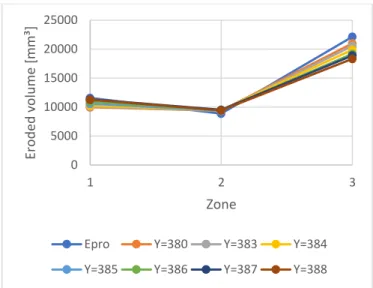
The results of the analysis in the y-direction are shown in Figure 7. The relative error is 9.7% in this case.
Figure 7. Sensitivity of the eroded volume of the inner ring to offset in the y-direction, test 39
The relative error in case of a shift in the vertical plane is naturally higher, however, this can be anticipated by shifting one of the profiles. The results of the sensitivity of the eroded volume of the inner ring to an offset of ± 1 mm is shown in Figure 8Figure 6 for test 39 of De Vos [1]. Z_base 0 denotes the original height of the raw data, while the others represent a shift of ± 1 mm of the data.
Figure 8. Sensitivity of the eroded volume of the inner ring to offset in the z-direction, test 39
Lastly, the relative error on the damage number due to the removal of points near the pile centre is analysed as well and lies in the same range as for the horizontal offset sensitivity analysis.
Considering all the analysed tests, the relative error on the damage number due to a shift in the horizontal plane ranges between 0.9% and 11.8% for the x-direction and between 0.5% and 13.4% in the y-direction. In the vertical direction the relative error ranges between 12.9% and 68.3%, however, this can easily be anticipated. The relative error due to the removal of points near the pile centre ranges between 3.8% and 13%. Generally, the absolute error range is similar for most tests. This yields a higher relative error in case of small damage tests.
0 5000 10000 15000 20000 25000 1 2 3 Ero d ed v o u m e [m m ³] Zone Epro X=3512 X=3513 X=3514 X=3515 X=3516 X=3517 X=3518 0 5000 10000 15000 20000 25000 1 2 3 Ero d ed v o lu m e [m m ³] Zone
Epro Y=380 Y=383 Y=384 Y=385 Y=386 Y=387 Y=388
0 5000 10000 15000 20000 25000 30000 1 2 3 Ero d ed v o lu m e [m m ³] Zone
C. Validation of the script
The results of the dry condition tests are promising, however, they still have to be validated with real data. The damage calculation of one of the tests executed by De Vos was compared for both methodologies for test 50. The reported S3D of test 50 of De Vos is 0.64. The damage number according to the re-analysed EPro data of this test is 0.63. The damage number calculated with the new post-processing script based on the raw EPro data is 0.67. This suggests that when the correct offset parameters are known, the new post-processing script can reproduce the results obtained by EPro within a tolerable range.
V. CONCLUSION
The two methodologies each have their own advantages and disadvantages. Generally, the handheld laser scanner can be used as a competitive alternative to EPro. It provides at least the same accuracy while being faster for smaller grid sizes. For a grid size of 5 mm and a relatively small area of interest, the two methods require approximately the same time, even though EPro can scan underwater. If a smaller grid size or large area of interest has to be scanned, the handheld laser scanner becomes significantly faster while still providing a higher resolution.
Especially in monopile scour protection experiments, the handheld laser scanner provides high efficiency of time spent in the wave flume. On the other hand, for larger scale breakwater experiments, the large dataset obtained with the handheld laser scanner is not necessarily needed and may result into a significantly longer processing time. However, this can be anticipated by tuning the grid size and the picking frequency without losing any accuracy.
ACKNOWLEDGEMENTS
The authors would like to acknowledge the support and suggestions of Prof. dr. ir. P. Troch, dr. ir. V. Stratigaki, M. Wu and C. A. Chavez.
REFERENCES
[1] De Vos, L., 2008. Optimisation of Scour Protection Design for Monopiles and Quantification of Wave Run-Up. Ghent University. [2] FARO®, 2017. FARO® Scanner Freestyle3D: User manual. URL
https://faro.app.box.com/s/pkfiiyeom0kwx722cff4yh01lwyspxu2/file/3 14135742270
[3] Meinert, P., 2006. EPro user manual. Department of Civil Engineering, Aalborg University. Hydraulics and Coastal Engineering, No. 39 [4] WindEurope, 2020. Offshore wind in Europe - Key trends and statistics
2019.
[5] Stratigaki, V., Todd, D., Whitehouse, R., Troch, P., 2019. Data storage report: Large scale experiments to improve monopile scour protection design adapted to climate change. Wallingford.
[6] Delafontaine, M., 2016. Experimental study on the performance of different wave absorbers in a wave flume.
[7] Chavez, C.E.A., Stratigaki, V., Wu, M., Troch, P., Schendel, A., Welzel, M., Villanueva, R., Schlurmann, T., De Vos, L., Kisacik, D., Pinto, F.T., Fazeres-Ferradosa, T., Santos, P.R., Baelus, L., Szengel, V., Bolle, A., Whitehouse, R., Todd, D., 2019. Large-scale experiments to improve monopile scour protection design adapted to climate change—the PROTEUS project. Energies 12. https://doi.org/10.3390/en12091709 [8] Hughes, S.A., 1993. Physical Models and Laboratory Techniques in
Coastal Engineering, Advanced Series on Ocean Engineering. World Scientific. https://doi.org/10.1142/2154
[9] Draycott, S., Steynor, J., Davey, T., Ingram, D.M., 2018. Isolating incident and reflected wave spectra in the presence of current. Coast. Eng. J. 60, 39–50. https://doi.org/10.1080/05785634.2017.1418798
ix
Table of contents
Chapter 1: Introduction ... 1
1.1 Offshore wind energy ... 1
1.2 The PROTEUS project ... 2
1.3 Objective and approach of the thesis ... 3
Chapter 2: Scour ... 4
2.1 Introduction ... 4
2.2 Sediment transport ... 4
2.2.1 Bed shear stress ... 5
2.2.2 Threshold of motion ... 11
2.3 Flow around a monopile foundation ... 14
2.3.1 Downflow in front of the pile ... 16
2.3.2 Horseshoe vortex... 17
2.3.3 Lee-wake vortex ... 21
2.3.4 Streamline contraction ... 23
2.3.5 Principles of scour protection ... 23
Chapter 3: Scale effects in physical hydraulic modelling ... 25
3.1 Introduction ... 25
3.2 Types of physical models ... 25
3.2.1 Fixed-bed models vs. movable-bed models ... 25
3.2.2 2D models vs. 3D models ... 26
3.2.3 Undistorted vs. distorted models ... 26
3.2.4 Site-specific vs. generic models ... 26
3.3 Hydraulic similitude ... 26 3.3.1 Similarity requirements ... 27 3.3.2 Froude criterion... 29 3.3.3 Reynolds criterion ... 30 3.3.4 Weber criterion ... 30 3.3.5 Cauchy criterion ... 30 3.3.6 Euler criterion ... 30 3.3.7 Strouhal criterion... 30 3.3.8 Conclusion ... 31
3.4 Achieving model-prototype similitude ... 33
3.4.1 Inspectional analysis ... 33
3.4.2 Dimensional analysis ... 33
3.4.3 Calibration ... 33
3.4.4 Scale series ... 33
3.5 How to deal with scale effects ... 34
3.5.1 Avoidance ... 34
3.5.2 Compensation ... 34
3.5.3 Correction ... 35
3.6 Transport models for scour ... 35
3.6.1 Hydrodynamic similitude requirements... 35
3.6.2 Sediment transport similitude requirements ... 36
3.6.3 Best Model ... 36
3.7 Expected scale effects in the scope of this thesis ... 38
Chapter 4: Wave flume set-up and procedure ... 40
4.1 Introduction ... 40
4.2 General description of the wave flume ... 40
4.3 Test conditions ... 41
4.3.1 Wave period and current velocity conditions ... 42
4.3.2 Water depth and wave height conditions ... 43
4.3.3 Scour protection characteristics ... 45
4.3.4 Overview of the target conditions ... 47
4.4 Set-up of the model ... 47
4.4.1 Sandbox construction ... 47
4.4.2 Passive wave absorption ... 48
4.4.3 Active wave absorption system ... 48
4.4.4 Measuring equipment ... 49
4.4.5 Model effects ... 51
4.5 Test procedure ... 51
4.6 Data analysis ... 52
4.6.1 Wave data analysis ... 52
4.6.2 Current data analysis ... 53
xi
Chapter 5: FARO® Freestyle3D handheld laser scanner... 56
5.1 Introduction ... 56
5.2 Using the FARO® Freestyle3D handheld laser scanner... 56
5.2.1 Available material ... 56
5.2.2 Calibration ... 58
5.2.3 Performing a scan... 59
5.3 Processing the scans in SCENE process ... 63
5.4 Manipulating the scans in CloudCompare ... 66
Chapter 6: Validation of damage calculation with the handheld laser scanner ... 76
6.1 Introduction ... 76
6.2 Problem statement ... 76
6.3 General description of the scripts ... 77
6.3.1 Conversion to grid data ... 77
6.3.2 Damage number calculation for handheld laser scanner ... 79
6.3.3 Damage number calculation for EPro... 82
6.4 Accuracy of handheld laser scanner measurements ... 82
6.4.1 Test of volume measurement ... 82
6.4.2 Grid size and picking frequency sensitivity analysis... 83
6.4.3 Sensitivity to offset ... 87
6.5 Accuracy of EPro measurements ... 89
6.5.1 Sensitivity to horizontal offset ... 90
6.5.2 Sensitivity to vertical offset ... 93
6.5.3 Sensitivity to Cr ... 94
6.5.4 Validation of the script with real data ... 95
6.6 Comparing the handheld laser scanner to EPro ... 96
Chapter 7: Conclusion ... 101
References ... 103
Appendix A: Test results ... 106
Appendix B: Logbook entries ... 126
List of figures
Figure 1-1: Belwind wind farm (Van Ginderdeuren, 2010) ... 1
Figure 1-2: Annual offshore wind installations by country and cumulative capacity (WindEurope, 2020) ... 2
Figure 2-1:Sediment transport processes (Soulsby, 1998) ... 4
Figure 2-2: Definition of the bottom boundary layer (Liu, 1998) ... 6
Figure 2-3: Non-linear interaction of wave and current bed shear stresses (Soulsby, 1998) ... 10
Figure 2-4: Forces acting on a grain (De Vos, 2008) ... 11
Figure 2-5: Adapted Shields curve, threshold of motion (Soulsby, 1998) ... 12
Figure 2-6: Modified Shields diagram (Hoffmans and Verheij, 1997) ... 13
Figure 2-7: Example of the amplification factor around a monopile exposed to a steady current (Sumer and Fredsøe, 2002) ... 14
Figure 2-8: Time development of scour depth (Sumer and Fredsøe, 2002) modified by Kortenhaus (2019) ... 15
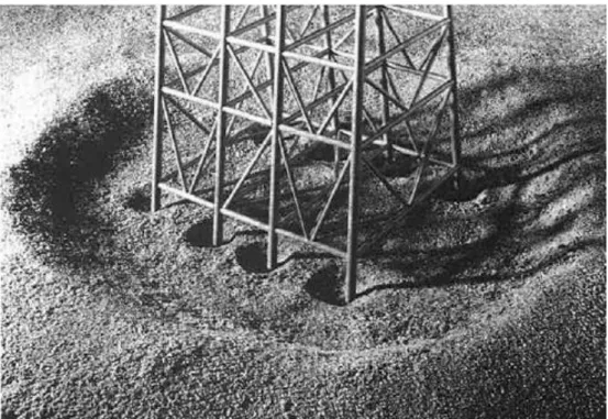
Figure 2-9: Scour around a piled steel jacket foundation (Sumer and Fredsøe, 2002), after Angus and Moore (1982) ... 16
Figure 2-10: Downflow upstream of a pile (Kortenhaus, 2019) ... 16
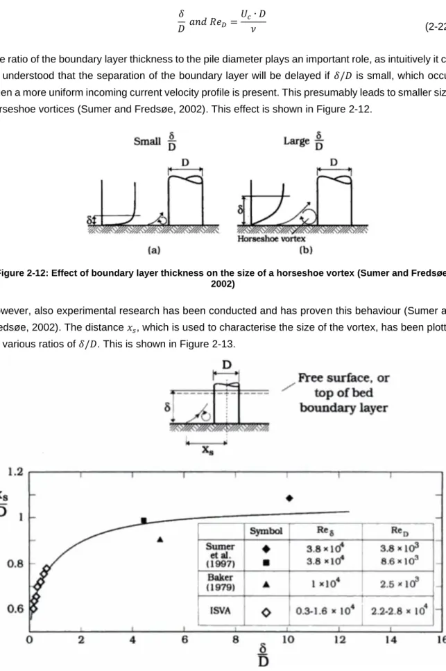
Figure 2-11: Definition sketch of the different hydrodynamic mechanisms (Sumer and Fredsøe, 2002) ... 17
Figure 2-12: Effect of boundary layer thickness on the size of a horseshoe vortex (Sumer and Fredsøe, 2002) ... 18
Figure 2-13: Influence of the boundary layer thickness on the separation distance xs (Sumer and Fredsøe, 2002) ... 18
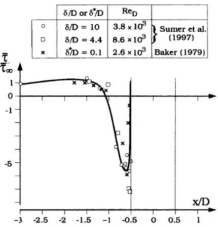
Figure 2-14: Bed shear stress induced by the horseshoe vortex upwards of the pile (Sumer and Fredsøe, 2002) ... 19
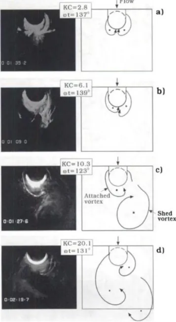
Figure 2-15: Creation of the horseshoe vortex due to waves (Sumer and Fredsøe, 1997) ... 20
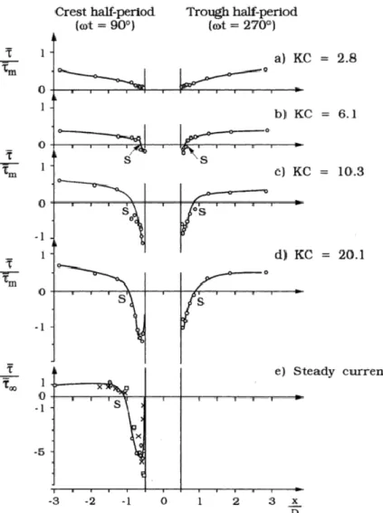
Figure 2-16: Amplification factor as a function of the KC number and the wave period cycle (Sumer and Fredsøe, 1997) ... 21
Figure 2-17: Near-bed wake vortices (Sumer and Fredsøe, 1997)... 22
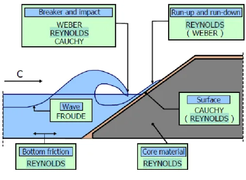
Figure 3-1: Similitude laws and scale effects when modelling wave loads in a sea dike (Troch et al., 2005) ... 29
Figure 4-1: Pump set-up ... 40
Figure 4-2: Current inlet ... 41
Figure 4-3: Overview of some of the executed tests during the PROTEUS project, modified from (Chavez et al., 2019) ... 41
Figure 4-4: Properties of the scour protections, (Chavez et al., 2019) ... 45
Figure 4-5: Downscaled rock gradings from the PROTEUS project for tests 10, 12 and 13 ... 45
Figure 4-6: Comparison between downscaled gradings and the proposed grading ... 46
Figure 4-7: Pile installed on the pile base using a transition piece (Loosveldt and Vannieuwenhuyse, 2012) ... 48
Figure 4-8: Detail of the positioning of the measuring equipment during the PROTEUS project (Stratigaki et al., 2019) ... 49
xiii
Figure 4-9: Top and side view of the wave flume set-up ... 50
Figure 4-10: Detail of the sandbox and placement of the measuring equipment ... 51
Figure 4-11: Wave gauge ... 52
Figure 4-12: Nortek Vectrino 3D Acoustic Velocimeter (Nortek AS, 2018) ... 53
Figure 4-13: ECM ... 53
Figure 4-14: Subzone definition (De Vos, 2008) ... 54
Figure 5-1: Available equipment ... 57
Figure 5-2: Components of the scanner ... 57
Figure 5-3: Markers ... 58
Figure 5-4: Opening SCENE capture ... 58
Figure 5-5: Entering the calibration plate number ... 58
Figure 5-6: Start of calibration ... 59
Figure 5-7: Calibration process ... 59
Figure 5-8: SCENE capture toolbar ... 60
Figure 5-9: SCENE capture settings ... 60
Figure 5-10: View on the tablet while scanning ... 61
Figure 5-11: Tracking lost ... 62
Figure 5-12: Processing in SCENE capture ... 62
Figure 5-13: Opening SCENE process ... 63
Figure 5-14: Selecting data to be transferred ... 63
Figure 5-15: General overview of the project ... 64
Figure 5-16: Viewing a scan in the explore tab ... 64
Figure 5-17: Export menu ... 65
Figure 5-18: Exporting the scans ... 65
Figure 5-19: General overview in CloudCompare ... 66
Figure 5-20: Loading a file ... 67
Figure 5-21: All scans have been loaded ... 67
Figure 5-22: Levelling a scan ... 68
Figure 5-23: Picking first point ... 68
Figure 5-24: Two points have been selected ... 69
Figure 5-25: Levelled scan ... 69
Figure 5-26: Point picking tool ... 70
Figure 5-27: Coordinates of the new origin ... 70
Figure 5-28: Setting the new origin ... 71
Figure 5-29: Confirmation of the new origin ... 71
Figure 5-30: Alignment tool ... 72
Figure 5-31: Selecting the refence scan ... 72
Figure 5-32: Alignment interface ... 73
Figure 5-33: The three reference points of the reference scan ... 73
Figure 5-34: End of selection process ... 74
Figure 5-35: Saving the file... 74
Figure 5-36: Saving options... 75
Figure 6-2: Negative peaks close to pile ... 77
Figure 6-3: Flowchart representing the working principle of the Python script ... 78
Figure 6-4: Top view of the point cloud of a scan of a scour protection before (left) and after (right) application of the Python script ... 79
Figure 6-5: Flowchart for the damage number calculation script for the handheld laser scanner ... 81
Figure 6-6: Definition of parameter Cr ... 82
Figure 6-7: Point cloud model of the wooden block ... 83
Figure 6-8: Initial profile of the scour protection during the dry condition test ... 84
Figure 6-9: Manually eroded profile of the scour protection during the dry condition test ... 84
Figure 6-10: Relative height difference map, grid size 3.5 mm, m=1 ... 86
Figure 6-11: Damage subdivision, grid size 3.5 mm, m=1 ... 86
Figure 6-12: Coordinate system definition of the second dry conditions test ... 87
Figure 6-13: Point cloud detail of the centre of the coordinate system of the dry conditions test ... 88
Figure 6-14: Cloud points near the centre of the pile on a scale of 1 mm ... 88
Figure 6-15: Sensitivity of the eroded volume of the inner ring to offset in the x-direction, test 5 ... 91
Figure 6-16: Sensitivity of the eroded volume of the inner ring to offset in the y-direction, test 5 ... 92
Figure 6-17: Sensitivity of the eroded volume of the inner ring to offset in the Z-direction, test 5 ... 93
Figure 6-18: Sensitivity of the eroded volume of the inner ring to Cr, test 5 ... 94
xv
List of tables
Table 3-1: Similitude ratios for Froude and Reynolds Similarity (Hudson et al., 1979) ... 32
Table 3-2: Bedload models (Hughes, 1993) ... 36
Table 4-1: Scaling of the peak wave period ... 43
Table 4-2: Scaling of the current velocity ... 43
Table 4-3: Scaling of the water depth ... 43
Table 4-4: Scaling of the significant wave height ... 44
Table 4-5: Wave-current interaction ... 44
Table 4-6: Scaling of the scour protection characteristics ... 45
Table 4-7: Sieving curve of the proposed rock grading ... 46
Table 4-8: Scour protection characteristics of the downscaled and the proposed grading ... 47
Table 4-9: Summary of the test conditions ... 47
Table 4-10: Scaled distances between centre of the pile and the considered wave gauges ... 49
Table 6-1: Volume measurement of wooden block ... 83
Table 6-2: Calculated volumes of the scanned wooden block ... 83
Table 6-3: Sensitivity analysis of the S3D damage number to grid size and picking frequency ... 85
Table 6-4: Sensitivity analysis of the damage number to horizontal pile offset ... 89
Table 6-5: Experimental conditions for the tests that will be used (De Vos, 2008) ... 90
Table 6-6: Sensitivity of S3D of the inner ring to offset in x-direction, test 5 ... 91
Table 6-7: Sensitivity of S3D of the inner ring to offset in y-direction, test 5 ... 92
Table 6-8: Summary of the sensitivity analysis to horizontal offset ... 92
Table 6-9: Sensitivity of S3D of the inner ring to offset in z-direction, test 5 ... 93
Table 6-10: Summary of the sensitivity analysis to vertical offset ... 94
Table 6-11: Sensitivity of S3D of the inner ring to Cr, test 5 ... 95
Table 6-12: Summary of the sensitivity analysis to Cr ... 95
Table 6-13: Analysis of test 50 in EPro ... 96
List of symbols and abbreviations
𝐴 = Amplitude of the horizontal wave motion [m]
𝐴𝐷𝑉 = Acoustic Doppler velocimeter [-]
𝐶 = Chézy resistance coefficient [m1/2/s]
𝐶𝑎 = Cauchy number [-]
𝐶𝑟 = Optimization parameter for EPro scan data [-]
𝐶𝑔,0 = Group velocity of a wave component in zero current [m/s]
𝐶𝑔,1 = Group velocity of a wave component in current [m/s]
𝐷 = Pile diameter [m]
𝐷𝑛50 = Nominal mean grain size diameter [m]
𝐷15 = The size of the grains at which 15% is finer [m]
𝐷50 = Mean grain diameter [m]
𝐷85 = The size of the grains at which 15% is finer [m]
𝐷∗ = Dimensionless grain size [-]
𝑑 = Water depth [m]
𝑑 = Sediment diameter [m]
𝑑50 = Average grain size of a grading [m]
𝑑𝑠 = Sediment grain diameter [m]
𝐸 = Young’s modulus [Mpa]
𝐸𝐶𝑀 = Electromagnetic current meter [-]
𝐸𝑢 = Euler number [-]
𝐹𝑟 = Froude number [-]
𝐹𝑟∗ = Densimetric Froude number [-]
𝐹𝐷 = Drag component of the hydrodynamic force [N]
𝐹𝐸 = Elastic compression force [N]
𝐹𝑔 = Gravitational force [N]
𝐹𝑖 = Inertial force [N]
𝐹𝐿 = Lift component of the hydrodynamic force [N]
𝐹𝑝 = Pressure force [N]
𝐹𝑠 = Reaction force that sediment particles exert on each other [N]
𝐹𝜇 = Viscous force [N]
𝐹𝜎 = Surface tension force [N]
𝑓 = Darcy-Weisbach resistance coefficient [-]
xvii
𝑓𝑤 = Wave friction factor [-]
𝑔 = Gravitational acceleration [m/s²]
𝐻 = Wave height [m]
𝐻𝑠 = Significant wave height [m]
𝐻0 = Wave height before wave-current interaction [m]
𝐻1 = Wave height after wave-current interaction [m]
ℎ = Water depth [m] 𝐾𝐶 = Keulegan-Carpenter number [-] 𝑘𝑆 = Bed roughness [m] 𝐿 = Length [m] 𝐿 = Wave length [m] 𝑙𝑠 = Relative length [-] 𝑁 = Number of waves [-]
𝑛 = Manning resistance coefficient [s/m1/3]
𝑝 = Pressure [Pa]
𝑅𝑒 = Reynolds number [-]
𝑅𝑒𝐷 = Pile Reynolds number [-]
𝑅𝑒∗ = Grain Reynolds number [-]
𝑆𝑡 = Strouhal number [-]
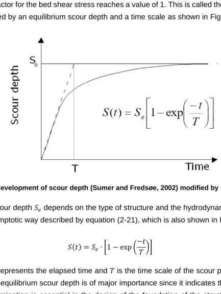
𝑆𝑒 = Equilibrium scour depth [m]
𝑆𝑠 = Relative sediment density [-]
𝑆(𝑡) = Function describing the development of scour depth over time [m]
𝑆3𝐷 = Three-dimensional damage number [-]
𝑆3𝐷,𝑠𝑢𝑏 = Three-dimensional damage number in the considered subzone [-]
𝑠 = Specific gravity [-]
𝑇 = Time scale describing the scour development rate [s]
𝑇𝑝 = Peak wave period [-]
𝑇𝑤 = Wave period [s]
𝑡 = Variable denoting the elapsed time [s]
𝑈 = Depth-averaged water velocity [m/s]
𝑈𝑟 = Ursell number [-]
𝑈𝑚 = Horizontal orbital velocity just above the seabed [m/s]
𝑈𝑐 = Steady current velocity [m/s]
𝑈(𝑧) = Local water velocity at depth z [m/s]
𝑢∗ = Friction velocity [m/s]
𝑢∗𝑐𝑟 = Critical friction velocity [m/s]
𝑉 = Velocity [m/s]
𝑉𝑒 = Eroded volume [m³]
𝑉𝜔 = Relative fall speed [-]
𝑣∗ = Shear velocity [m/s]
𝑊 = Submerged unit weight of a sediment particle [N]
𝑊𝑒 = Weber number [-]
𝑋̅ = Weighted average of parameter 𝑋 [variable]
𝑥𝑠 = Distance from the creation of the horseshoe vortex to the pile centre [m]
𝑧0 = Roughness length [m]
𝛼 = Amplification factor for the bed shear stress [-]
𝛾 = Specific weight [N/m³]
𝛾𝑖 = Submerged sediment specific weight [= (𝜌𝑠− 𝜌)𝑔 ] [N/m²s²]
𝛿 = Thickness of the boundary layer [m]
𝜃 = Shields parameter [-]
𝜃𝑐𝑟 = Critical Shields parameter [-]
𝜅 = Von Kármán constant [-]
𝜆 = Characteristic length [m]
𝜆𝑋 =
Scale ratio of the parameter X, defined as 𝑋𝑝/𝑋𝑚, with 𝑋𝑝 the value of 𝑋
in the prototype, and 𝑋𝑚 the value of 𝑋 in the model
[-]
𝜇 = Dynamic viscosity [Pa.s]
𝜈 = Kinematic viscosity [m²/s]
𝜌 = Density [kg/m³]
𝜌𝑠 = Density of sediment [kg/m³]
𝜌𝑤 = Density of water [kg/m³]
𝜎 = Surface tension [N/m]
𝜏∞ = Bed shear stress without the presence of a pile, in the same hydraulic conditions as with the pile [N/m²]
𝜏𝑏 = Bed shear stress [N/m²]
𝜏𝑏,𝑐 = Bed shear stress due to the current [N/m²]
𝜏𝑏,𝑤 = Bed shear stress due to the waves [N/m²]
𝜏𝑐,𝑤 = Bed shear stress due to the combination of current and waves [N/m²]
xix
𝜏𝑚 = Mean bed shear stress due to the combination of current and waves [N/m²]
𝜏𝑚𝑎𝑥 = Maximum bed shear stress due to the combination of current and waves [N/m²]
𝜙 = Angle between the main direction of the waves and the current [rad]
𝜓 = Alternative notation of Shields’ parameter [-]
𝜔 = Oscillation frequency [Hz]
Chapter 1: Introduction
1.1
Offshore wind energy
Renewable energy has become more and more popular over the last few decades. The most important reason for this is climate change. The CO2 from the combustion of fossil fuels is the leading contributor in greenhouse gas emissions. The ensuing global warming has caused governments and companies to invest heavily in renewable energy. One such source of renewable energy is wind energy. Wind turbines can be placed both onshore or offshore. Protest from people who do not want a wind turbine in their backyard and the higher wind speeds at offshore locations make offshore wind energy an attractive energy source, as the latter leads to more electricity generation per amount of capacity installed. A local example is the Belwind wind farm on the Bligh Bank near the port of Zeebrugge, as depicted on Figure 1-1.
Figure 1-1: Belwind wind farm (Van Ginderdeuren, 2010)
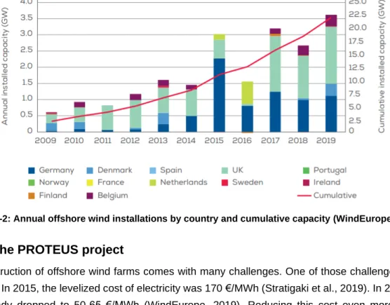
According to the annual report of WindEurope (2020), 3623 MW of net offshore capacity has been added in 2019 in Europe, corresponding to 502 new offshore wind turbines. The average rated capacity of turbines installed in 2019 was 7.8 MW, a 1 MW increase compared to 2018. Figure 1-2 shows a clear increase in yearly installed capacity over the last decade. At the end of 2019, 5047 offshore wind turbines were connected to the grid in total, corresponding to a total capacity of 22.1 GW across 110 wind farms in 12 countries, making Europe the world leader in offshore wind power. The UK, Germany, Denmark, Belgium and the Netherlands are the most relevant players in the European offshore wind energy market and are responsible for 98.6% of the cumulative capacity. Also the rated capacity of the wind turbines, the wind farm sizes, the water depth and the distance to shore have greatly increased over the last decade, even though most wind turbines are bottom fixed (WindEurope, 2020).
When looking at the substructures and foundations, monopiles are the most popular. 70% of all newly-installed foundations in 2019 were monopiles, while 84.37% of all offshore wind turbine foundations in Europe are monopiles (WindEurope, 2020). Yearly total investments in offshore wind energy in Europe in the last decade ranged from €5 billion in 2012 to €18.2 billion in 2016 (WindEurope, 2020). This
indicates that offshore wind farms are quite costly, highlighting the importance of optimization of offshore wind turbines and their foundations.
Figure 1-2: Annual offshore wind installations by country and cumulative capacity (WindEurope, 2020)
1.2
The PROTEUS project
The construction of offshore wind farms comes with many challenges. One of those challenges is the high cost. In 2015, the levelized cost of electricity was 170 €/MWh (Stratigaki et al., 2019). In 2018, this cost already dropped to 50-65 €/MWh (WindEurope, 2019). Reducing this cost even more makes offshore wind energy more accessible. In case of a monopile, the foundation makes up around 20% of the total costs (Stratigaki et al., 2019). To ensure the safety of the wind turbine structure and reduce the installation cost, the design of the foundation is crucial. When exposed to waves and currents, the wind turbine foundation faces the risks of scouring. Therefore, an armour layer protection is usually applied to prevent scouring around the monopile foundation. This scour protection makes up a large part of the costs of the foundation. It is therefore of great importance that the design of this scour protection is optimized.
Besides optimizing the scour protection, the extension of the lifetime of an offshore wind turbine can also reduce the costs. To make this possible, the long term damage behaviour of the scour protection around the monopile should be investigated. As previously mentioned, also the impact of climate change should be investigated, as this will lead to increased design storms.
Based on these motivations, the European Hydralab+ PROTEUS (PRotection of Offshore wind Turbine monopilEs against Scouring) project was founded. The project focussed on large-scale physical modelling of monopile foundations in the Fast Flow Facility (FFF) at HR Wallingford. This infrastructure supports a test scale of 1:8.33. The project aims to optimize the design of scour protection around offshore wind turbine monopiles, as well as shielding them against the future impacts of climate change (Chavez et al., 2019). The main research objective is to establish a basic benchmark dataset on the stability of scour protection around monopile foundations to serve as a basis for model tests in other wave flumes in the future (Stratigaki et al., 2019). In the collaborative spirit of the Hydralab+ project, the project has multiple partners from all over Europe: Department of Civil Engineering at Ghent University,
HR Wallingford (UK), the Ludwig-Franzius Institute for Hydraulic, Estuarine and Coastal Engineering at the University of Hannover, the Faculty of Engineering at the University of Porto, the Geotechnics division of the Belgian Department of Mobility and Public Works, and International Marine and Dredging Consultants (IMDC nv).
1.3
Objective and approach of the thesis
The analysis of the PROTEUS experiments has shown that scale effects are not accounted for in the current design practices. A downscaling of the experiments performed during the PROTEUS project will allow the quantification of the scale effects and help improve the design practices.
The main objective of this research was initially to perform experiments in the large wave flume in the Coastal Engineering Research Group (CERG) of Ghent University. The study would have been done by downscaling the experimental test programme accomplished during the PROTEUS project. The experiments consider a scour protection around a monopile foundation under the combined action of waves and currents. The initial goals of the thesis were:
• An advanced literature study on the failure of scour protections and scale effects; • a thorough analysis of the reference dataset of the PROTEUS project;
• the design, set-up and execution of tests in the large wave flume of the Coastal Engineering Research Group;
• post-processing of the obtained data in terms of the scour protection damage and hydrodynamic loads;
• a comparison between the reference and obtained dataset; • a critical evaluation of the obtained results and methods.
As mentioned in the preamble, the actual physical modelling tests in the wave flume had to be cancelled for the safety of everyone involved. Due to these unforeseen circumstances, the objective of the thesis was changed around the 15th of March to the following:
• An advanced literature study on the failure of scour protections and scale effects; • a thorough analysis of the reference dataset of the PROTEUS project;
• the design and set-up of test in the large wave flume of the Coastal Engineering Research Group;
• re-analysis of S3D damage of data from De Vos (2008) using a correction of the pile offset, using a new script, for a selected number of tests;
• a detailed study of the FARO® Freestyle3D handheld laser scanner, with a description of the procedure for future use, with a study of the achieved accuracy.
Chapter 2: Scour
2.1
Introduction
Flowing water, whether in a pipeline, open channel or sea, causes friction at the interface between the water and the boundary it flows over. If such a surface is made of a monolithic material such as concrete or steel, that surface will only be subjected to small shear stresses caused by the flow. However, in case of a moveable bed, which is most often the case for a marine environment, the different sediment particles that make up the boundary are not strongly bound to each other. This makes it possible that some of these sediment particles are eroded, which alters the shape of the interface and hence the bed configuration. These particles are then transported by the flow and deposited elsewhere. This is called sediment transport. The presence of a monopile in a current field disturbs the flow of water. This disturbance is characterised by a sudden change in flow patterns and leads to increased sediment transport around the pile. This phenomenon is called scour. In this thesis, scour around a monopile will be studied by conducting small-scale tests. Scour damages the scour protection around the monopile. This has direct consequences with respect to the lifetime of a wind turbine. Therefore, this chapter is dedicated to describing the principles that play a role in the scour development around monopiles. Firstly, the basic principles of sediment transport will be discussed. In this discussion, the effect of a current and/or waves in the absence of any object perturbing the flow is treated. This will be followed by a summary of the research concerning the flow patterns around a single, slender vertical monopile in a combined wave and current regime and how this affects the local sediment transport.
2.2
Sediment transport
Scour is defined as the removal of sediment from around an object. This removal is due to a nonequilibrium in the sediment transport. More sand is being transported away than there is accreted, resulting into a net loss of sand material at that particular location. In a turbulent marine environment, sand can easily be stirred up and then carried away by a tidal, wind or wave driven current. It eventually ends up being deposited somewhere farther down the stream. Soulsby (1998) refers to this as the entrainment, transportation and deposition of sediment, which is illustrated in Figure 2-1. These three processes are continuously interacting with each other and occur simultaneously.
Entrainment of sediment particles is the result of destabilizing forces being larger than the stabilizing gravitational forces. The destabilizing forces result into bed shear stresses and are the product of friction exerted by the (wave-induced) current and by the lift component of the hydrodynamic load. The theory of the threshold of motion particularly addresses the physics behind particle entrainment and will be discussed more thoroughly in section 2.2.2.
Once the particles are entrained, they are transported away by means of rolling, hopping and sliding along the bed. This mode of transportation is called the bed load and is the dominant mode of transportation in case of a small current or in case of large grains (Soulsby, 1998). Another method of transportation is the suspended load. This occurs when particles are small enough or when the current is large enough (Soulsby, 1998). In this case, fine material is put into suspension and consequently transported away by the current. Whether bed load or suspended load predominates depends on the grain sizes that are encountered in the studied environment. In a marine environment, grains coarser than 2 mm will usually be transported as bedload and grains finer than 0.2 mm as suspended load (Soulsby, 1998).
Depending on the settling velocity and flow conditions, grains will eventually come to rest after having travelled a certain distance. Grains transported as bedload will stop rolling and sliding and suspended grains will settle down. Both processes of entrainment and deposition can occur simultaneously at the same location (Soulsby, 1998).
The rate at which sediment is transported away at a particular location is the determining factor for scour development. The widely used definition of the sediment transport rate mentioned by Soulsby (1998) is the amount of sediment passing through a vertical plane of unit width perpendicular to the flow direction per unit of time. The amount of sediment can either be expressed as mass or as volume. It should be noted, however, that a high sediment transport rate does not necessarily mean that scour should be expected. If both the supply and the removal of sediment are high but of the same magnitude, the sediment transport rate will be high, but the level of the bed will not significantly change. Scour around a monopile can thus only develop if there is an nonequilibrium between the supply and removal rate (Soulsby, 1998).
For the calculation of the sediment transport rate in a particular cross section, the hydrodynamic boundary conditions, consisting of the current velocity profile, the potential influence of waves and the composition of the bed material, should be analysed. Different formulas exist to calculate the sediment transport rate for both the suspended load and the bed load. These can be found in Liu (1998). These formulas are particularly interesting for sediment mobility studies. For the scope of this thesis, the induced bed shear stress is the most important parameter as it determines whether particles will be entrained. Therefore, the rest of this section is dedicated to the determination of the bed shear stress and the theory of initiation of motion.
2.2.1 Bed shear stress
The abovementioned hydrodynamic loads exert friction on the seabed. This frictional force is most often expressed per unit area of the seabed and is called the bed shear stress 𝜏𝑏. For mathematical
convenience, however, mostly the friction velocity 𝑢∗ is used. This parameter is defined as (Soulsby,
𝑢∗= √
𝜏𝑏
𝜌𝑤
(2-1)
In equation (2-1), 𝜌𝑤 represents the density of water. 𝑢∗ should not be regarded as a physical velocity.
It can, however, be linked to the turbulent fluctuations in the real velocity components (Soulsby, 1998). Dimensionless parameters are useful, as they can be used to compare similar processes of different magnitudes. The bed shear stress and consequently the friction velocity are made dimensionless by relating them to the weight of the sediment in the vicinity of the flow. This dimensionless representation is called the Shields parameter 𝜃, which represents the ratio of the load acting on a grain to its resistance to movement due to its weight. In case the bed shear stress is used, the Shields parameter is defined as (Shields, 1936):
𝜃 = 𝜏𝑏
𝑔 ∙ (𝜌𝑠− 𝜌𝑤) ∙ 𝑑𝑠 (2-2)
In case the friction velocity is used, it can be defined as (Shields, 1936):
𝜃 = 𝑢∗²
𝑔 ∙ (𝑠 − 1) ∙ 𝑑𝑠
(2-3) In equation (2-2), 𝑔 represents the acceleration due to gravity, 𝜌𝑠 the density of the sediment grains and
𝑑𝑠 the sediment grain diameter. In equation (2-3), 𝑠 represents the specific density of the sediment
grains, which is the ratio of the densities of sediment and water.
The presence of the bed disturbs the flow of water near the bottom. It is the disturbed flow that plays a dominant role when analysing sediment transport. This disturbed flow is called the boundary layer flow and is found in the bottom boundary layer (Soulsby, 1998). Qualitatively, this boundary layer is defined as the layer inside which the flow is significantly influenced by the bed. A more quantitative and commonly accepted definition is the distance from the bed to the point where the velocity is 99.5% of the steady current 𝑈𝑐 (Liu, 1998). The latter is depicted in Figure 2-2.
In shallow water, where the presence of waves and the corresponding orbital velocities is felt at the level of the bed, additionally an oscillatory boundary layer exists. Due to its oscillating nature, the lifetime and consequently the thickness of the boundary layer is smaller compared to the boundary layer of a steady current. However, the bed shear stress is larger for smaller boundary layer thicknesses for the same free stream velocity 𝑈𝑐 (De Vos, 2008). As the capacity of the flow to transport sediment mainly depends
on the bed shear stress and not on the layer thickness itself, waves tend to predominate in the particle entrainment process (De Vos, 2008). However, for the transportation of the entrained sediment, current is still the dominating mechanism since the orbital velocity induced by the waves is oscillatory and does not transport particles over long distances (Nielsen, 1992).
In this thesis, the combined effect of waves and current on a scour protection is investigated. However, before analysing the combined effect, their individual contributions are discerned and discussed first.
2.2.1.1 Bed shear stress induced by the current
Marine currents can have many different origins. They can be induced by tidal motion, wind, atmospheric pressure gradients, water surface slopes and density gradients (Soulsby, 1998). Nearshore, the most important current contribution is from the wave-induced longshore current (Soulsby, 1998). Today, monopiles can also be found farther offshore where a combination of tidal and meteorological effects tend to dominate.
In shallow or transitional water, the boundary layer can occupy a major part of the water column. In this boundary layer, the current increases from zero at the bottom to a maximum just below the water surface. A velocity profile describes the fluctuation of the current velocity as a function of the water depth. Most often, the depth-averaged current speed is used as the characteristic value and is defined as (Soulsby, 1998): 𝑈𝑐= 1 𝑑∫ 𝑈(𝑧) 𝑑𝑧 𝑑 0 (2-4) In equation (2-4), 𝑈(𝑧) represents the velocity profile and d the water depth. However, the lower limit of the integral in equation (2-4) is most often not zero but equal to 𝑧0, which is the bed roughness length.
Intuitively, it can be understood that a sand bed is not perfectly flat and that it has a certain roughness. The quantity 𝑧0 captures this and depends on the viscosity of the water, the current velocity and the
natural roughness of the bed. It is defined as (Christoffersen and Jonsson, 1985):
𝑧0= 𝑘𝑠 30[1 − exp (− 𝑢∗𝑘𝑠 27𝜈)] + 𝜈 9𝑢∗ (2-5)
In which 𝑘𝑠 is the physical bottom roughness and 𝜈 the kinematic viscosity of water. A simplified and
frequently used version of equation (2-5) has been suggested by Colebrook and White (1937):
𝑧0= 𝑘𝑠 30+ 𝜈 9𝑢∗ (2-6)
Equation (2-6) can be even further simplified when considering hydrodynamically rough or smooth flow. However, Soulsby (1998) mentions that it is common practice to treat all flows over sand as
𝑧0=
𝑘𝑠
30 (2-7)
Soulsby (1998) reports a simplification error of less than 10% for grains larger than 60 μm.
The bottom roughness 𝑘𝑠 is often related to the grain size of the sediment. Many relations between 𝑘𝑠
and a characteristic grain size have been proposed, however, the most widely used relationship is (Soulsby, 1998):
𝑘𝑠= 2.5 𝑑50 (2-8)
In which the 𝑑50 is the average grain size of the sediment grading.
Another parameter of equation (2-4) is the velocity profile 𝑈(𝑧). Most often the profile is assumed to be logarithmic, which is expressed as (Soulsby, 1998):
𝑈(𝑧) =𝑢∗ 𝜅 ln
𝑧
𝑧0 (2-9)
In which 𝜅 is the von Kármán constant. The value of this constant is 0.40, even for marine currents and suspended particles (Soulsby, 1998). De Vos (2008) mentions that for a hydraulically rough flow, in which the boundary layer is established over the entire water depth, the depth averaged velocity is found at a depth of about 0.4d above the water bed.
The bed shear stress induced by the current is related to the depth-averaged velocity through (De Vos, 2008):
𝜏𝑏,𝑐=
1 2𝜌𝑤𝑓𝑐𝑈𝑐
2 (2-10)
In which 𝑓𝑐 is the friction coefficient of the bed. Different formulas of this friction coefficient exist,
introduced by different hydraulic engineers. These are calculated using different coefficients. The most well-known coefficients are the Darcy-Weisbach resistance coefficient 𝑓, the Chézy coefficient C and the Manning coefficient 𝑛. Caution is advised when using friction coefficients as it is not always clear which formulation has been used.
Equation (2-10) is only valid for a flat seabed without any ripples, dunes or sandwaves, as it only represents the bed shear stress due to skin friction. However, these are the most common marine conditions outside of the surf zone (Soulsby, 1998). Therefore, the bed shear stress will not only be composed of the skin friction introduced in equation (2-10), but also of a form-drag component due to the pressure field acting on the ripples or other seabed modifications. The sum of both leads to the total bed shear stress due to a current (Soulsby, 1998).
2.2.1.2 Bed shear stress induced by the waves
Waves create different forms of current, for example longshore current and undertow. Furthermore, asymmetry exists between the velocity profile found underneath a wave crest and the one underneath a wave trough. This leads to an important source of net sediment transport (Soulsby, 1998). In order for
waves to disturb the seabed, the water has to be sufficiently shallow. This means that, at the bottom, the orbital velocity underneath the wave has to be larger than 0. This is usually the case in shallow water, where the relative water depth d/L is smaller than 0.05, and in transitional water, where d/L is between 0.05 and 0.5. An important remark is that the orbital velocities are oscillatory and change sign every half wave period. The orbital velocity just above the bed 𝑈𝑚 can be derived using linear wave
theory and is valid for transitional and shallow water (De Vos, 2008): 𝑈𝑚=
𝜋𝐻 𝑇𝑤
∙ 1
sinh (2𝜋𝑑𝐿 ) (2-11)
In which 𝑇𝑤 is the wave period, 𝐻 the wave height, and 𝐿 the wave length. This bottom velocity leads to
a boundary layer due to the same frictional effects as a normal current. However, this boundary layer is oscillatory and its thickness is significantly smaller. The order of magnitude of this boundary layer is ranging from millimetres to centimetres. This is because the flow is reverting before the boundary layer can grow to a significant length (De Vos, 2008). Consequently, larger shear velocities can be reached in the wave boundary layer, which in turn causes a higher bed shear stresses (De Vos, 2008; Soulsby, 1998).
The bed shear stress caused by waves 𝜏𝑏,𝑤 is calculated as (De Vos, 2008):
𝜏𝑏,𝑤 =
1
2𝜌𝑤𝑓𝑤𝑈𝑚
2 (2-12)
In equation (2-12), 𝑓𝑤 represents the wave friction factor. Many different expressions are found in
literature for the wave friction factor (Fredsøe and Deigaard, 1992; Myrhaug, 1989; Nielsen, 1992; Soulsby and Whitehouse, 1997).
Similar to the current only case, waves generally do not travel in seas with a perfectly flat bottom. Especially in shallow water, ripples, dunes or sandwaves can be present and lead to an increased bed shear stress similar as in the case of a current. Also for waves, a form-drag component is added to the skin friction component calculated by equation (2-12) to account for this (Soulsby, 1998).
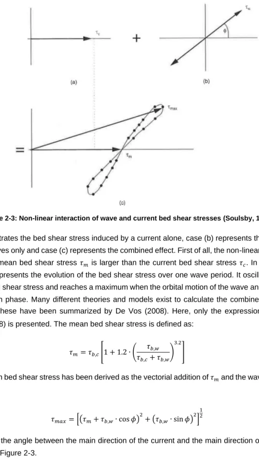
2.2.1.3 Combination of waves and current
In this thesis, the combined effect of waves and current is studied since waves and current occur together in most parts of the continental shelf and thus around offshore structures. The study of the combined effect of waves and current is more complicated because they hydrodynamically interact with each other in such a way that their combined effect is non-linear (Soulsby, 1998). Consequently, the individual contributions of each of the components, cannot just simply be added to each other. This non-linear behaviour is due to the modification of the phase speed and wavelength of the waves caused by the current. This causes waves to be slightly refracted (Soulsby, 1998). The boundary layers formed by the waves and current also interact with each other, which leads to an enhancement of the bed shear stress (Soulsby, 1998). Only the boundary layer interaction is dealt with here.
Several studies regarding the near-bed velocities and stresses in a combined regime have been conducted (Delgado Blanco et al., 2004; Umeyama, 2005). From these studies, De Vos (2008) summarized that for waves following a current there is a reduced current near the free surface and for