Non-linearity in the NOx/NO2 conversion

Non-linearity in the NO

_x

/NO

₂

conversion

Report 680705009/2008

RIVM Report 680705009/2008

Non-linearity in the NO

_x

/NO

₂

conversion

J. Wesseling, RIVM F. Sauter, RIVM Contact: Joost Wesseling RIVM/LVM Joost.Wesseling@rivm.nl

This investigation has been performed by order and for the account of Ministry of VROM, within the framework of the project Urban Air Quality, project M/680705/07.

RIVM

National Institute for Public Health and the Environment P.O. Box 1

3720 BA Bilthoven The Netherlands

© RIVM 2008

Parts of this publication may be reproduced, provided acknowledgement is given to the 'National Institute for Public Health and the Environment', along with the title and year of publication.

Abstract

Non-linearity in the NOx/NO2 conversion

The yearly average NO2 concentration along roads is influenced by the way it is calculated. The RIVM has analyzed the mathematical relations involved of some of the models being used in the Netherlands. With this information, the differences between model calculations as well as between models and experimental data can be understood in a better way.

On locations with a lot of traffic the yearly average limit value for NO2 is exceeded regularly. In the Netherlands compliance with EU air quality regulations is usually checked using the results of model calculations. The models being used in the Netherlands calculate the NO2 concentrations in several ways. It is long known that different calculation schemes produce different results. So far, the exact reasons for this were not known. By analyzing the relations that are used, the relations between calculation schemes haven been determined and the differences haven been quantified.

The relations between different calculation schemes have been determined for several locations of the National Air Quality measuring Network of the RIVM in the Netherlands, where yearly average concentrations are being measured. The specific location where the yearly average NO2 is calculated, especially the type of buildings along the street and the orientation of the street, appears to have a complex influence on the relation between several calculation schemes. At present not enough field data is available to determine the relations between calculation schemes for all of the Netherlands.

Rapport in het kort

Niet-lineariteit in de NOx/NO2 conversie

De wijze waarop de jaargemiddelde concentratie stikstofdioxide langs wegen wordt berekend, beïnvloedt de uitkomst. Het RIVM heeft de onderliggende wiskunde geanalyseerd van rekenmodellen die hiervoor in Nederland worden gebruikt. Met deze kennis kunnen de onderlinge verschillen tussen rekenmodellen onderling en tussen rekenmodellen en metingen beter worden begrepen.

Op locaties met veel verkeer wordt de gemiddelde concentratie stikstofdioxide die jaarlijks wettelijk is toegestaan vaak overschreden. In Nederland wordt deze jaargemiddelde concentratie stikstofdioxide vaak niet gemeten maar met behulp van modellen berekend. De hiervoor gebruikte modellen berekenen de jaargemiddelde concentratie stikstofdioxide op verschillende manieren. Het was al bekend dat dit tot uiteenlopende resultaten kan leiden, alleen waren de onderliggende redenen onbekend. Door de

wiskundige relaties te analyseren, is aangetoond op welke manier de rekenwijzen van verschillende modellen met elkaar samenhangen en hoe de verschillende uitkomsten kunnen worden

gekwantificeerd.

De relaties tussen de rekenwijzen zijn bepaald voor enkele locaties van het Landelijk Meetnet Luchtkwaliteit van het RIVM waar de jaargemiddelde concentraties worden gemeten. De locatie, vooral de bebouwing langs de straat en de ligging van de straat, blijkt invloed te hebben op de wijze waarop de rekenwijzen samenhangen. Er zijn momenteel te weinig meetgegevens beschikbaar om de wiskundige relaties tussen de verschillende rekenwijzen voor geheel Nederland in kaart te brengen.

Contents

Summary 6 1 Introduction 9 2 Global analysis 11 2.1 Analysis 11 2.2 Comparison to measurements 15 2.2.1 Urban situations 15 2.2.2 Rural situation 21 3 Conclusions 23 3.1 General conclusions 23

3.2 Values of the correction factors 24

References 27

Most frequently used symbols 29

Appendix 1 Detailed analysis 31

Appendix 2 NOx/NO2 conversion in CAR; history 49

Appendix 3 Sensitivities 53

Appendix 4 Calibration of SRM-1 57

Summary

In the Netherlands several models are used to determine the NO2 concentrations along roads. These models typically consist of a part that calculates the basic dispersion of pollutants (i.e. NOx), while the effect on the NO2 concentrations is then determined using an additional model. Most of the current Dutch models employ a rather simple NOx/NO2 conversion scheme. The relation between NOx concentrations and NO2 concentrations is non-linear. Due to this non-linearity, the value of the yearly averaged concentration contribution of traffic will depend on the way it is calculated. The averaged value can be obtained in three ways:

A. from the average value of all hourly calculated concentrations contributions; B. from calculated yearly averaged NOx and O3 contributions;

C. from calculated yearly averaged NOx and O3 contributions within wind sectors.

At least three effects have to be taken into account when determining the yearly averaged NO2 concentration: (1) the non-linearity of the photo-chemical conversion function, (2) correlations between the contributions of traffic to NO emissions and O3 background concentrations and (3) model deficiencies. The mathematical relations involved have been analyzed by the RIVM. With these, the differences between calculation schemes as well as between models and experimental data can be understood in a better way.

A correction factor has been defined to compensate for the effect of using either method B or C instead of the normal method A. A second correction factor was defined to correct for the model deficiencies. The values of the correction factors have been determined for several locations of measuring stations of the RIVM. The correction factors have been shown to depend on the distribution of NO concentrations as well as on the correlation between the NO concentrations and the O3 background concentrations, the shape and orientation of the street as well as the exact location within a street will – to some extent – influence the values of the correction factors. These factors probably explain the relatively large variations in the values obtained for the correction factors. The consequence of such variations is that it is not currently possible to suggest using average correction factors for areas throughout the Netherlands. Furthermore, the available data are not sufficient to determine the pattern of the variations with an accuracy required to estimate their values in general situations.

The influence of the surroundings is, by definition, small in the case of a highway through an open field. However, here also the correlation between the NO and O3 concentrations will be important. Again, not enough data is available to suggest average correction factors that can be used throughout the Netherlands.

The research presented in this report has focussed on the NOx/NO2 conversion model as it is presently used in several Dutch models. In principle, the same kind of analysis can be applied to other conversion schemes. Further research in this field will be conducted by the RIVM.

The authors would like to thank Karel van Velzen (MNP), Hans Erbrink (KEMA) and Ernst Meijer (TNO) for their comments on an early draft of this report.

1

Introduction

The most important legal limit value for nitrogen dioxide (NO2) is the yearly averaged concentration. A legal limit value for the maximum hourly NO2 concentration also exists, but in the Netherlands this limit value is practically never exceeded (Beijk et al., 2007). In the Netherlands several models are used to determine the NO2 concentrations along roads. These models typically consist of a part that calculates the basic dispersion of pollutants (i.e. NOx), while the effect on the NO2 concentrations is then determined using an additional model. Most of the current Dutch models [Standard Calculation Model, SRM-1 for urban streets (also known as CAR) and SRM-2 for highways] employ a rather simple NOx/NO2 conversion scheme.

The relation between NOx concentrations and NO2 concentrations is non-linear. In this report the effect of this non-linear chemical relation on the yearly averaged concentration of NO2 contributed by road traffic will be discussed. Due to this non-linearity, the value of the yearly averaged concentration contribution of traffic will depend on the calculation:

− as the average of all individual hourly values calculated for every hour;

− calculated from the yearly averaged concentration of NO or NOx contributed by traffic, in combination with the yearly averaged ozone (O3) concentration;

− calculated from a wind rose of yearly averaged concentrations of NO or NOx contributed by traffic, in combination with a wind rose of yearly averaged O3 concentration.

2

Global analysis

2.1

Analysis

The total production of NO2 due to traffic emissions is the result of two processes – the direct emission of NO2 by vehicles and the reaction of emitted NO with O3, the so-called photo-conversion reaction. The average direct emission of NO2 in 2007 amounts to 7% of the NOx emitted by medium-duty and heavy-duty vehicles together and roughly 18% of that emitted by smaller cars. The total NO2 concentration in the close vicinity of a road therefore consists of three parts:

total NO2 = directly emitted NO2 + NO2 converted from NO + background.

The timescale of the photo-chemical reaction is in the order of several minutes. As meteorological conditions and background levels are usually assumed to be roughly constant during a 1-hour period, it would appear to be a reasonable assumption that a chemical steady-state condition exists during each 1-hour interval. The non-linearity in the averaging of the NO/NO2 conversion is due to the photo-chemical reactions. Ozone is formed when various pollutants react under the influence of sunlight. NO molecules from the exhaust of cars and trucks react with this ozone to form NO2. This process is called photo-conversion, and it can be described in a model using a mathematical function. We will denote the photo-conversion function by

g

(

n

_i

,

o

_i

)

(in μg/m3), where ni stands for the amount of NO (μg/m3) that is available during the 1-hour measuring interval, and oi represents the background concentration of O3 during that hour (also in μg/m3). The following general assumptions can be made for the photo-conversion function:

− the function values, i.e. concentration of converted NO2 are positive: i i i i

o

n

o

n

g

(

,

)

≥

0

∀

,

(1)

− the slope of the function is positive, with more NO leading to more converted NO2: i i i i i

o

n

n

o

n

g

,

0

)

,

(

∀

>

∂

∂

(2)

− with increasing NO concentrations the relative amount of converted NO2 decreases due to O3 limitation: i i i i i

o

n

n

o

n

g

,

0

)

,

(

2 2

∀

<

∂

∂

. (3)

The relation between the available amounts of NO and converted NO2 is roughly as shown in Figure 1, below. 0 5 10 15 20 25 30 0 50 100 150 200

n

g(

n

,o)

40

Figure 1 Typical relation between the amount of NO and converted NO2.

The Dutch standard calculation model 2 (SRM-2), which is used along highways and large provincial roads, employs a very simple empirical relation, originally proposed by Van den Hout (1988), for the photo-chemical conversion:

K

n

n

o

o

n

g

i i i i i

+

=

.

)

,

(

(4)

where the index i denotes a specific hour, and the function

g

(

n

i

,

o

i

)

represents the amount of NO2 that

is converted, given a certain NO traffic contribution (ni) and a specific O3 background (oi) The empirical constant K is assumed to have a value of 100 and, by definition, the same unit as the concentrations. The value of K was obtained from a comparison of measured and calculated NO2 concentrations. The amount of NO, denoted by ni, is a fraction of the amount of NOx (≡NO + NO2), with ni = (1-f ) NOx(hour=i), with f denoting the fraction of NO2 emitted directly by the vehicles. In this report, the term ‘concentrations’ indicates ‘concentration contributions from traffic’. All concentrations are given in micrograms per cubic meter and NOx concentrations are in units of NO2. The term

‘conversion concentration’ indicates the amount of NO2 that was converted from NO into NO2 in a photo-chemical reaction with O3.

As an example of the non-linear nature of averaging, let us assume a constant O3 background concentration of 40 μg/m3_{. Given NO}

x concentrations of 10, 100 and 190 μg/m3 during three 1-hour periods, respectively, the average value is 100 μg/m3_{. For these same 3 hours the function}

₍

_,

₎

i

i

o

n

g

has values of 3.6, 20.0 and 26.2 μg/m3 _{respectively, with an average of 16.6 μg/m}3_{. If}

₍

_,

₎

i

i

o

n

g

is

evaluated using the average NOx and O3 concentrations of 100 and 40 μg/m3 the result is 20 μg/m3. Clearly, the result of averaging the three hourly NO2 concentrations (16.6) is not equal to the NO2 concentration obtained from the average NOx and ozone concentrations; as demonstrated, they differ by a factor of 16.6/20.0 = 0.83. In practice there are much more hours with lower NOx contributions than there are hours with (very) high NOx contributions and the non-linearity can be substantially larger. For a more general analysis of the above, we will initially assume (a) that relation (4) provides a good description of the hourly NOx /NO2 conversion process and (b) that there is a constant amount of O3 during the entire year.

We will denote the yearly averaged value of the function g( ) by1_:

)

,

(

n

_i

o

_i

g

. (5)

The average value of all hourly values ni is denoted by

n

. The function value of

n

is given by

)

,

( o

n

g

. (6)

Given the shape of the function g(ni, o), with the assumptions (1)–(3), it is clear that for all concentration contributions Δ > 0:

g(

n

+Δ, o) - g(

n

, o) < g(

n

, o) - g(

n

-Δ, o). (7)

In case there are at least as many hours with ni<

n

as there are hours with

n

<ni we can deduce:

)

,

(

)

,

(

n

o

g

n

o

g

>

. (8)

Generalizing (8) to also include the effect of variations in O3, we can write:

1 _{A bar indicates time-averaging, usually over 1 year. When different averaging periods are used, these will be clearly}

χ

⋅

=

(

,

)

)

,

(

n

o

g

n

o

g

(9)

A more detailed analysis is presented in Appendix 1. The factor

χ

is shown to compensate for the average effect of both the non-linearity of the model and the effect of correlations between the NOx contributions of the traffic and the O3 background concentrations. This value depends on the distribution of the values for ni and oi. Once the distributions for the NOx and O3 concentrations are obtained, the value of

χ

can be calculated (see Appendix 1). The RIVM has a measuring station (LML639, see Beijk et al.,2007) in the ‘Erzeijstraat’, a typical street canyon, that is located in the city of Utrecht. Using the measured distributions of NO contributions and O3 background concentrations measured there in the year 2003 the value of

χ

can be calculated to be 0.66. The measuring station LML640, Universiteitsbibliotheek, was used as a background station.

Thus far we have assumed that (hourly) model results are in good agreement with actual field measurements. In the case of a flawed model, however, (systematic) differences between calculated and measured concentrations may occur. When comparing calculated NO2 conversion contributions to measured values we therefore need to introduce an additional correction factor:

θ

⋅

=

(

,

)

)

,

(

n

o

g

n

o

g

_measured . (10)

The parameter

θ

is the result of several effects, the non-linearity of the model as well as possible model deficiencies. From (9) and (10) we also define a correction factor for model deficiencies

α

. Whereas the value of

χ

can be calculated and the value of

θ

can be determined from a comparison between calculated and measured concentrations, the value of

α

can not be determined directly. It is defined as follows:

χ

θ

α

=

. (11)

The values of

α

and

θ

depend on many factors and are hard to estimate. For example, the NOx background concentration does not influence the result of the conversion function (4), whereas calculations with the chemistry package of OSPM, a practical street pollution model, do indicate an influence. As a result of these mechanisms the values of

θ

and

α

may vary both in time and location and, as a result, compared to

χ

they are much harder to calculate (see Appendix 1). The Dutch CAR model contains an empirically derived value of

θ

= 0.6 that has been derived from geometrical considerations and a comparison to a limited amount of experimental data (Eerens et al., 1993; see Appendix 2). Given the measured NO contributions of the traffic and measured O3 backgrounds for the Erzeijstraat in 2003, we can calculate the correction factor

θ

in a semi-analytical way, deriving a value of 0.71, with

χ

= 0.66; this results in a value of 1.08 for

α

. Using a different procedure, which

is outlined in Appendix 1, the values of

α

and

θ

can also be derived directly from hourly measurements and calculations. We then obtain

χ

= 0.66,

θ

= 0.70 and

α

= 1.06. Although calculated in a different way, the values are in good agreement.

In a number of situations, dispersion models are used to calculate the concentration contributions for a number (usually 12) of wind directions and/or wind sectors. The yearly averaged concentration is then obtained from a weighted average of the sectors. The correction factors

α

_S ,

χ

_S and

θ

_S (the subscript

S indicates averaging over wind sectors) can also be determined for the case of discrete wind sectors.

The variation in O3 concentrations within each sector is smaller than the variation over the full 360 degrees. In addition, the variation in NOx contributions within each sector will usually be smaller and the correlation between the NOx and O3 will be different from that of the general case. Therefore, the results of such an analysis using wind sectors will differ from the general results that are obtained neglecting wind sectors.

2.2

Comparison to measurements

The correction factors can be determined from field measurements in cases where the NOx and NO2 contributions from traffic can be determined. This means that pairs of measuring stations are needed, one inside a street or next to a highway and one in a location that is representative of the background concentration. The contributions from traffic can be obtained from the concentration differences measured at these locations. Unfortunately, only a few such pairs of measuring stations are available in the Netherlands.

2.2.1

Urban situations

The values of

χ

,

θ

and

α

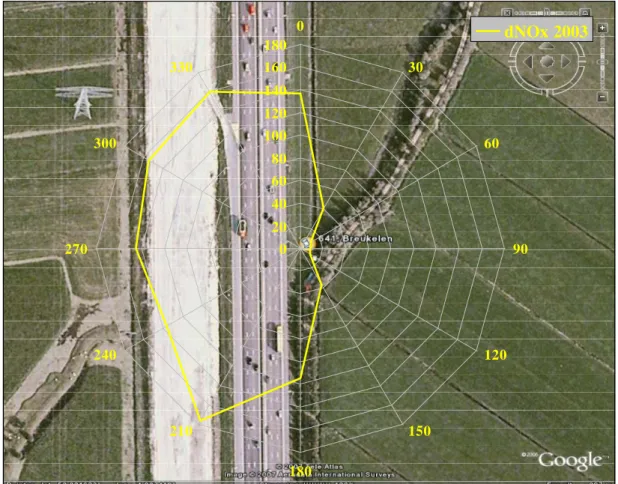
have been calculated and compared to measurements for three locations with measuring stations of the RIVM – one in a street canyon in a busy city (Utrecht: Erzeijstraat) and two near intersections of roads (Groningen: Europaweg; Nijmegen: Graafseweg). A detailed analysis for the Erzeijstraat is presented in Appendix 1. The procedure for the Europaweg and the Graafseweg is identical. In Utrecht also a measuring station is available on the Kardinaal de Jongweg. Unfortunately, the background location of Universiteitsbibliotheek does not seem to be representative for the location of the Kardinaal de Jongweg. Therefore, the data from these stations could not be combined.

In Figure 2 the wind rose of NOx concentration contributions measured at the measuring station in the Erzeijstraat, weighted with the chance of occurring, is shown for 2003. The meteorological data are taken from Schiphol.

0 20 40 60 80 100 120 0 30 60 90 120 150 180 210 240 270 300 330

dNOx 2003

Figure 2 Wind rose of NOx concentration contributions in the Erzeijstraat. LML640 was

used as the background location.

For the general case of yearly averaged concentrations, the values for

χ

,

θ

and

α

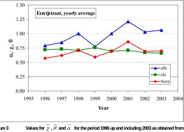
have been determined from the available data for 1996–2003 using MATLAB, version 7. The results are plotted in Figure 3.

Erzeijstraat, yearly average 0.00 0.25 0.50 0.75 1.00 1.25 1.50 1995 1996 1997 1998 1999 2000 2001 2002 2003 2004 Year

α,

χ

,

θ

alfa chi theta

Figure 3 Values for

χ

,

θ

and

α

for the period 1996 up and including 2003 as obtained from field data of the RIVM.

The value of

χ

varies only slightly from year to year, between 0.66 and 0.77. In comparison, the value of

θ

varies substantially more – between 0.57 and 0.86, with an average value of 0.68. The average value for the period 2000–2003 is somewhat higher at 0.74. As already mentioned, the values for

θ

must be compared to the value of 0.6 that is currently used in the SRM-1 model. The value of

α

varies between 0.78 and 1.21.

The results presented in Figure 3 were obtained neglecting the variations between wind sectors. The values averaged for wind rose are presented in Figure 4 for the period 1996–2003.

Erzeijstraat, sectors 0.00 0.25 0.50 0.75 1.00 1.25 1.50 1995 1996 1997 1998 1999 2000 2001 2002 2003 2004 Year

α

s , χ

s , θ

s

alfa chi theta

Figure 4 Values for

θ

_S ,

α

_S and

χ

_S in the Erzeijstraat in the period 1996–2003.

Although the shapes of the curves in Figure 4 are quite similar to those in Figure 3, the values of the correction factors

θ

_S are up to 8–12% higher than those obtained in the general case. In the wind rose-averaged case, the value of

χ

_S varies between 0.72 and 0.78, that of

θ

_S varies between 0.57 and 0.95, with an average value of 0.73, and the average value for

θ

_S over the period 2000–2003 is, as in the field data, somewhat higher at 0.82. Data are still available for the Erzeijstraat measuring station, but in 2003 the background measuring station in Utrecht (‘Universiteitsbibliotheek’) was rendered inoperative. As a result, it has not been possible to analyse NO2 conversion in recent years.

More recently, new background/street station combinations have been commissioned in Groningen, Nijmegen and Breda. The street station in Breda does not provide data for NO2 and NOx; however, 3 and 4 years of valid data are available for Groningen and Nijmegen, respectively. The data from these latter two locations have been used to perform analyses similar to those carried out on the Erzeijstraat datasets. As there are no O3 measurements available for the street locations in Nijmegen and Breda, it has not been possible to determine the direct NO2 emission from the field measurements. A value based on traffic emission factors was therefore calculated, which resulted in a relatively high uncertainty in the values of

θ

_S and

α

_S . The value of

χ

_S can be determined with a higher accuracy as this parameter

is not very sensitive to the value of the direct NO2 fraction (see Appendix 3). The results of the analyses are shown in Figures 5 and 6.

Yearly average 0.40 0.60 0.80 1.00 1.20 1.40 1.60 2003 2004 2005 2006 2007 2008 Year

θ

an

d

χ

theta, Graafseweg theta, Europaweg chi, Graafseweg chi, Europaweg alfa, Graafseweg alfa, Europaweg

Figure 5 Values for

θ

,

χ

and

α

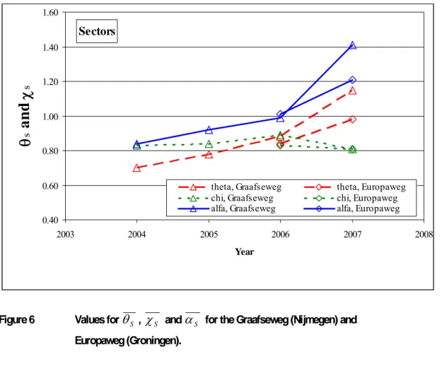
for the period 2004 up to and including 2007 for the Graafseweg (Nijmegen) and Europaweg (Groningen).

Sectors 0.40 0.60 0.80 1.00 1.20 1.40 1.60 2003 2004 2005 2006 2007 2008 Year

θ

s

an

d

χ

s

theta, Graafseweg theta, Europaweg chi, Graafseweg chi, Europaweg alfa, Graafseweg alfa, Europaweg

Figure 6 Values for

θ

_S ,

χ

_S and

α

_S for the Graafseweg (Nijmegen) and Europaweg (Groningen).

The values for the correction factors

θ

and

θ

_S and, therefore, also for

α

and

α

_S increase substantially in 2007, but the reason for this is not clear. The correction factors

χ

and

χ

_S for the locations in Groningen and Nijmegen are also approximately 12–22% higher than those obtained for the Erzeijstraat. Given the underlying mathematical structure of χ, these differences may be due to the street canyon type of the Erzijstraat versus the much more open character of the other locations. The result of these differences is that the distribution of NOx contributions as well as the correlation between the NOx and ozone will be different. The values for

θ

and

θ

S and also those of

α

and

α

S are roughly comparable to those obtained in the Erzijstraat. The yearly variation in these values is quite substantial.

Wesseling and Sauter (2007) carried out a calibration study of the SRM-1 model in 2007 and observed that the calculated values of the NO2 contribution at the Groningen and Nijmegen locations substantially underestimated the measured values. These contributions were calculated using the standard setting of SRM-1, in which the amount of converted NO2 is scaled by a factor of 0.6. Based on the analyses reported here, it would appear that this value of 0.6 is not suitable for these locations and that values of 0.80 (Groningen) and 0.84 (Nijmegen) would be more appropriate. This supposition was

verified when these latter values were used in the calibration instead of 0.60, and a better agreement was subsequently found between calculated and measured NO2 contributions, see Appendix 4.

2.2.2

Rural situation

Figure 7 shows the 2003 wind rose of NOx contributions that were determined at measuring station LML641, located close to Breukelen. The meteorological data are taken from Schiphol.

0 20 40 60 80 100 120 140 160 180 0 30 60 90 120 150 180 210 240 270 300 330

dNOx 2003

Figure 7 The wind rose of NOx contributions at the LML641 measuring station (Breukelen) in 2003.

The measuring station is situated directly beside a busy highway, the A2, which, at that location, runs almost perfectly north–south. Some 150,000 vehicles pass the station each day, of which roughly 10% consist of medium-duty and heavy-duty traffic vehicles.

A detailed analysis of the Breukelen location is presented in Appendix 1. For the case of wind sector-averaged concentrations, the values for

α

_S ,

χ

_S and

θ

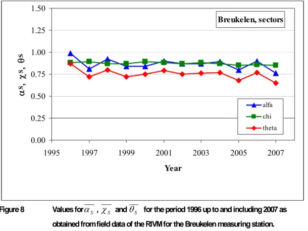
_S (for the wind sectors influenced by the road

emissions) are determined from the available data for 1996 to 2007 using MATLAB, ver. 7. The results are plotted in Figure 8.

Breukelen, sectors 0.00 0.25 0.50 0.75 1.00 1.25 1.50 1995 1997 1999 2001 2003 2005 2007 Year

α

S

, χ

S

, θ

S alfa chi theta

Figure 8 Values for

α

_S ,

χ

_S and

θ

_S for the period 1996 up to and including 2007 as obtained from field data of the RIVM for the Breukelen measuring station.

.

The values can be seen to be quite constant over the whole period. The value of

θ

_S varies slightly, with an average value of 0.75; the value of

α

_S also varies slightly, with an average value of 0.87. The value of

χ

_S is practically constant at 0.87.

3

Conclusions

3.1

General conclusions

The objective of this report was to demonstrate how the exact value of the calculated yearly averaged value of the NO2 contribution of traffic is influenced by the approach used to determine its value. This averaged value can be obtained in three ways:

A. from the average value of all hourly calculated concentrations contributions; B. from calculated yearly averaged NOx and O3 contributions;

C. from calculated yearly averaged NOx and O3 contributions within wind sectors.

At least three effects have to be taken into account when determining the yearly averaged NO2 concentration: (1) the non-linearity of the photo-chemical conversion function, (2) correlations between the contributions of traffic to NO emissions and O3 background concentrations and (3) model deficiencies.

A correction factor

χ

has been used to compensate for the effect of using either method B or C instead of the ‘normal’ method A;

χ

corrects the effect of averaging the non-linear photo-chemical

conversion function. A second correction factor,

α

, corrects the model deficiencies (in the case of an ideal model,

α

= 1); it is used in all three methods mentioned above. The overall correction factor is

θ

=

α

χ

. The values of the correction factors have been determined for several locations of measuring stations of the RIVM. The value of

χ

seems quite stable in time for each location. The values of

θ

, and therefore also of

α

, can change substantially over time.

As the correction factors have been shown to depend on the distribution of NO concentrations as well as on the correlation between the NO concentrations and the O3 background concentrations, the shape and orientation of the street as well as the exact location within a street will – to some extent – influence the values of the correction factors. These factors probably explain the relatively large variations in the values obtained for the correction factors. The consequence of such variations is that it is not currently possible to suggest using average correction factors for areas throughout the Netherlands. An additional factor is that available data are not sufficient to determine the pattern of the variations with an accuracy required to estimate their values in general situations.

The influence of the surroundings is, by definition, small in the case of a highway through an open field. However, here also the correlation between the NO and O3 concentrations will be important.

Again, not enough data is available to suggest average correction factors that can be used throughout the Netherlands.

The research presented in this report has focussed on the NOx/NO2 conversion model as it is presently used in several Dutch models. In principle, the same kind of analysis can be applied to other conversion schemes. Further research in this field will be conducted by the RIVM.

3.2

Values of the correction factors

Ad A.

For method A, it is important to determine how well the calculated concentrations are in agreement with reality (field measurements). An average correction factor,

α

, can be defined to describe how well the model calculations and measurements agree. For the location of the Erzeijstraat in Utrecht, the NO2 conversion routine being used in the Dutch model SRM-2 requires values of

α

between 0.78 and 1.21 for the years from 1996 up to and including 2003, with an average of 0.96. Concentrations determined using method A are unbiased and do not need any corrections for non-linearity in obtaining the yearly averaged NO2 concentration due to traffic.

Ad B.

For method B, which is used in the Dutch SRM-1 model, model deficiencies also have to be corrected for. An additional factor that must be considered is the important effect of the non-linearity of the photo-chemical conversion. A correction factor,

χ

, can be derived for this effect, and in several urban situations that have been investigated it varies between 0.66 and 0.90 in the period 1996–2007. When model deficiencies of SRM-1 are also taken into account, the overall correction factor

θ

varies between 0.57 and 1.11. The value for the overall correction must be compared to the value of 0.6 that is used in the Dutch SRM-1.

Ad C.

For method C, the same points should be taken into account as when using method B. The variation in O3 concentrations is smaller within each sector than that over the full 360 degrees. In addition, within each sector the variation in NOx contributions will usually be smaller and the correlation between the NOx and O3 will be different from the general case. For urban locations, the value of

χ

_S (weighted average over all wind sectors S) varies between 0.72 and 0.89. The value of

θ

_S varies between 0.57 and 1.15.

Using method C for a highway through an open field results in values for the correction factors that are quite constant in time. The value of

θ

_S varies slightly between 0.65 and 0.87, with an average value of 0.75. Similarly, the value of

α

_S varies slightly between 0.76 and 0.99, with an average value of 0.87. The value of

χ

_S is practically constant at 0.87.

References

Beijk R, Mooibroek D and Hoogerbrugge R, Air quality in the Netherlands, 2003-2006, in Dutch, RIVM report 680704002, 2007.

Carslaw DC and Beevers, SD, ‘Investigating the potential importance of primary NO2 emissions in a street canyon’, Atm. Env. 38 (2004) 3585–3594.

Eerens, HC, Sliggers, CJ and Hout, KD van den, ‘The CAR model: The Dutch Method to Determine City Street Air Quality’, Atm. Env. 27B, no. 4, 389-399, 1993.

Hout, D. van den, and Baars, HP,’ Ontwikkeling van twee modellen voor de verspreiding van luchtverontreiniging door verkeer: Het TNO-verkeersmodel en het CAR-model’, in Dutch, TNO R88/192, 1988.

Teeuwisse SD. ‘CAR II: Aanpassing van CAR aan de nieuwe Europese richtlijnen’, TNO rapport 2003/119, 2003.

Vissenberg HA, en Velze K van, ‘Handleiding CAR-AMvB programma (versie 2.0)’, RIVM rapport 722101035, 1998.

Wesseling JP and Sauter FJ, ‘Calibration of the program CAR II using measurements of the national measuring network of the RIVM’, in Dutch, RIVM report 680705004, 2007.

Most frequently used symbols

α (n, o) correction factor to compensate for model deficiencies (no units)

) (S

α

average value of the correction factor for model deficiencies (no unit); the subscript S indicates averaging within one wind direction sector )

(S

β

the average value of the correction factor for the effect of averaging the NO part of the non-linear conversion function (no unit)

) (S

χ

the average value of the correction factor for the effect of averaging the NO and O3 parts of the non-linear conversion function (no unit)

) (S

θ

the average value of the combined effect of the corrections factors for model deficiencies and averaging the non-linear function (no unit)

cim the measured amount of converted NO2 in hour i (μg/m3) cic de calculated amount of converted NO2 in hour i (μg/m3)

m S

c

the average measured amount of converted NO2 (in wind sector S) (μg/m3) c

S

c

the average calculated amount of converted NO2 (in wind sector S) (μg/m3)

f the fraction of NO2 directly emitted by traffic (no unit)

)

,

(

n

j

o

j

g

the (assumed) photo-chemical conversion function (no unit)

H(n, o) the number of hours within a year having an NO contribution n and

an O3 background concentration of o (no unit)

)

,

(

x

μ,σ,δ

F

log normal function with parameters

μ

,

σ

,

δ

(no unit)

K conversion constant with empirical value of 100

i

n

the NO traffic contribution within hour i (μg/m3)

n

the yearly averaged NO concentration (μg/m3)

i

o

the O3 traffic contribution within hour i (μg/m3)

Appendix 1 Detailed analysis

Introduction

The example in chapter 2 illustrates the difference in the result due to the order of the operations – first calculating the NOx/NO2 conversion versus first calculating the yearly averaged concentrations. Given a set of values {ni} during a 1-year period, with an average value

n

, we can define a set of hourly factors {βi} by which g(ni,o) differs from g(ni,o). This can be written as:

)

(

)

(

)

,

(

)

,

(

)

(

K

n

n

K

n

n

o

n

g

o

n

g

n

i i i i i

+

+

=

=

β

(A1-1)

The average correction factor

β

, given by the ratio of

g

( o

n

,

)

and

g

( o

n

,

)

, can be written as the average correction factor βi(ni) for each possible value of ni, weighted by the chance of occurring (F):

∑

=

=

j j j i

n

F

o

n

g

o

n

g

)

(

)

,

(

)

,

(

_β

β

(A1-2)

The frequency distribution for the NOx contributions is needed to be able to calculate the value of

β

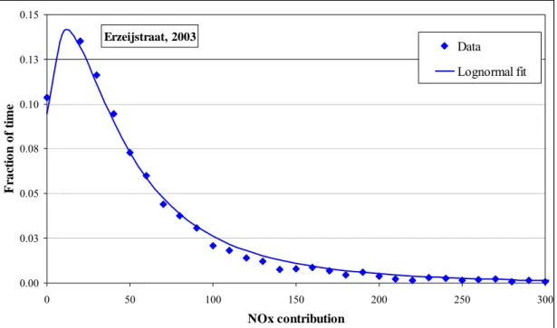
. This can be obtained from the field measurements. Figure A-1 shows the frequency of observed NOx concentration contributions:

Erzeijstraat, 2003 0.00 0.03 0.05 0.08 0.10 0.13 0.15 0 50 100 150 200 250 300 NOx contribution F ra ct ion of t im e Data Lognormal fit

Figure A1-1 Distribution of NOx concentration contributions as measured in the Erzeijstraat.

Location LML640 was used to provide the background levels.

The frequency distribution F( ) closely follows a three-parameter lognormal distribution given by:

π σ δ σ μ δ δ σ μ 2 ) ( ) ln( 2 1 , , 2

)

,

(

₊ ⎟ ⎠ ⎞ ⎜ ⎝ ⎛ + − −

=

x x

e

x

F

(A1-3)

with x being the NOx contributions and δ, μ and σ being the shape parameters of the distribution. The average NOx contribution is ( + ) 2

+

=

δ

μ 2σ 1

e

x

. For the above data the values δ = 10, μ = 3.86 and σ = 0.88 yield a satisfactory description of the data2_{. The total correction factor can now be written as:}

∫

=

F

(

x

)

β

(

x

)

dx

β

(A1-4)

Using relations (10) and (11), this can be written as

∫

−

₊

+

+

₋

₊

₊

=

+ − + − + max 2 2 2 2 0 0.5 / ) ) (ln( 5 . 0 5 . 0

)

)(

)

1

(

)(

(

)

)

)(

1

((

2

2

1

N _x

dx

x

K

f

x

e

e

K

e

f

x

δ

δ

π

σ

δ

β

_μμ _σσ δ μ σ (A1-5)

with Nmax being the maximum NOx concentration contribution that can reasonably occur. The integral has been evaluated using the shape parameters obtained from the fit and a value of 0.66 obtained. This factor compensates for the fact that the yearly averaged NO2 calculated from individual hours yields a result that differs from a yearly averaged NO2 calculated from yearly averaged NOx and O3 concentrations.

The numerical effect of averaging the NOx with varying O3

The amount of converted NO2 depends on the amount of available O3. The effect of the O3 can be included in our analysis. The amount of converted NO2 for an hourly NO concentration nj and an hourly ozone concentration oj is given by:

K

n

n

o

o

n

g

i i i i i

+

=

.

)

,

(

(A1-6)

Using relation (9) we can write the above:

NO2 (conversion part) =

β

(

n

i

).

g

(

n

,

o

i

)

(A1-7)

The effect of the O3 can be written as a function of the actual hourly value and the yearly averaged value (o):

K

n

n

o

o

n

o

n

g

i i i i

+

⋅

⋅

=

(

)

(

)

.

)

,

(

β

γ

(A1-8)

with β given by (9) and

γ

is defined as:

o

o

o

i i

)

=

(

γ

(A1-9)

Although

g

(

n

i

,

o

i

)

is directly proportional to γ, non-linear effects in the averaging procedure can not

be excluded due to a possible correlation between β and γ. The calculated yearly average conversion contribution can be obtained from a direct summation:

⎟⎟

⎠

⎞

⎜⎜

⎝

⎛

⋅

=

⎟⎟

⎠

⎞

⎜⎜

⎝

⎛

⋅

+

=

∑

∑

= = i allhours i i hours all i i i

n

o

M

o

n

g

o

n

M

K

n

n

o

o

n

g

(

,

)

.

1

β

(

)

γ

(

)

(

,

)

1

β

(

)

γ

(

)

(A1-10)

with M being the number of (valid) hours in a year. Equation (17) can also be written as:

i i

o

n

g

o

n

g

(

,

)

=

(

,

)

⋅

β

⋅

γ

∑

∑

−

⋅

−

=

⋅

⋅

−

⋅

−

⋅

+

⋅

⋅

i i i i i i i i

M

o

n

g

M

o

n

g

(

,

)

1

(

β

δβ

)

(

γ

δγ

)

(

,

)

1

(

β

γ

δβ

γ

β

δγ

δβ

δγ

)

From the definitions, it follows that

δβ

i

=

δγ

i

=

0

,

γ

=

1

and that the sum can be written as:

⎟

⎠

⎞

⎜

⎝

⎛

₊

_⋅

⋅

=

⋅

+

⋅

∑

∑

i i i i i i

M

o

n

g

M

o

n

g

(

,

)

1

(

β

δβ

δγ

)

(

,

)

β

1

δβ

δγ

(A1-11) We ultimately obtain:

(

i i

)

i i

o

g

n

o

n

g

(

,

)

=

(

,

)

⋅

β

+

δβ

⋅

δγ

(A1-12)

Therefore, in addition to the basic non-linearity of β, the possible correlation between β and γ further complicates the relation between hourly concentrations and the yearly average. Such a correlation can occur, for example, when the street is located such that the concentration contribution from the traffic is large for those wind directions for which the O3 background is also large. If there is no correlation, then by definition,

δβ

_i

⋅

δγ

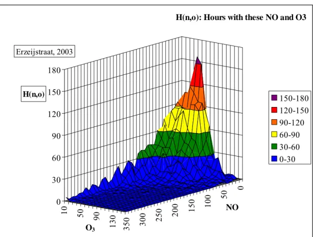
_i=0.

We describe the number of hours in a year with NO contribution n and O3 background concentration o by a distribution H(n, o). The measured distribution function H(n, o) for the Erzeijstraat in 2003 is presented in Figure A1-2. Both the O3 concentrations and NO contributions are in steps of 10 μg/m3.

0 50 100 150 200 250 300 350 10 ₅₀ 90 130 0 30 60 90 120 150 180 H(n,o) NO O3

H(n,o): Hours with these NO and O3

150-180 120-150 90-120 60-90 30-60 0-30 Erzeijstraat, 2003

Figure A1-2 Distribution of the number of hours in the Erzeijstraat in 2003 with specific values for the O3 and NO contribution.

With H(n, o), the yearly average conversion contribution can also be rewritten as a sum over all possible values of the NO and O3:

∑ ∑

= =

⋅

=

NOx j k ozone k j k j

o

n

o

n

H

M

o

n

g

o

n

g

(

,

)

(

,

)

1

(

,

)

β

(

)

γ

(

)

(A1-13)

From the above it is clear that the correction factor depends on a number of factors, with

γ

(

o

_k

)

taking into account the O3 dependency of the correction, a function

β

(

n

j

)

taking into account the NO (or NOx) dependency of the correction and a function

α

(

n

j

,

o

k

)

taking into account possible deficiencies of the underlying model which, in this case, is given by relation (4). The distribution H(n,o) will vary somewhat from year to year, mainly due to meteorological and traffic variations. We can write Equation (A1-13) as

χ

⋅

=

(

,

)

)

,

(

n

o

g

n

o

g

(A1-14) with:

∑∑

⋅

⋅

=

j k k j k j

o

n

o

n

H

M

(

,

)

(

)

(

)

1

_β

_γ

χ

(A1-15)

Using the definitions

∑∑

=

j k jk

H

M

1

1

,

=

∑∑

⋅

=

∑∑

⋅

j k k jk j k j jk

H

M

H

M

β

γ

γ

β

1

,

1

(A1-16)

the above can also be written as:

∑∑

∑∑

⋅

+

⋅

⋅

=

⋅

+

=

i k i i jk j k j jk i i

H

M

H

M

β

δβ

δγ

δγ

δβ

β

χ

1

1

(A1-17)

The factor

χ

is equal to the ratio of the yearly averaged amount of converted NO2 calculated from individual hourly concentrations and the yearly averaged amount of converted NO2 calculated from yearly averaged NO and O3 concentrations, assuming the conversion model to be correct. The factor

χ

depends on the structure of the conversion model (A1-6) and on the distribution of – and correlation between – the NO contributions and O3 concentrations.

For the example of the Erzeijstraat in 2003, we find the following correlation:

.

66

.

0

,

163

.

0

,

13

.

0

,

79

.

0

⋅

=

−

⋅

=

−

+

⋅

=

=

i i _{i i} i i

β

β

δβ

δγ

δγ

δβ

δγ

δβ

β

In the Dutch model SRM-1, a fitted value of 0.6 is used for the expression

β

+

δβ

_i

⋅

δγ

_i.

The concentration contribution is usually defined as the difference between the concentration in the street and the concentration at a nearby city background location. The theory still applies if, for some reason, a city background concentration is not available and a large-scale regional concentration is used; however the values for H(n,o) and, therefore, also for

χ

will then be different.

Model performance

So far we have assumed that (hourly) model results are in good agreement with reality – i.e. with field measurements. In the case of a flawed model, however, (systematic) differences between the calculated and measured concentrations may occur. We therefore define an hourly function αι() that is the ratio

between the measured and calculated NO2 conversion concentration contribution. The function αι()

may depend on many parameters or conditions. With this function included in the calculations, we can write the expression for the yearly averaged

NO

2 conversion concentration as:

∑

⋅

⋅

=

i i i i bg i i

n

nox

n

o

f

M

o

n

g

o

n

g

(

,

)

(

,

)

1

α

(

,

,

_,

,...)

β

(

)

γ

(

)

(A1-18)

The summation runs over all hours. Assuming α( ) depends mainly on nj and ok, we can rewrite Equation (A1-18) as a sum over all possible NO and O3 concentrations:

∑∑

⋅

⋅

⋅

=

j k k j k j k j

o

n

o

n

o

n

H

M

o

n

g

o

n

g

(

,

)

(

,

)

1

(

,

)

α

(

,

)

β

(

)

γ

(

)

(A1-19)

The value of

χ

does not depend on whether the conversion model is correct or not. In the case where the model for calculating the hourly amount of converted NO2 is not (fully) correct for all hours, we can write a similar relation for the correction factor

θ

:

∑ ∑

= =

⎟

⎠

⎞

⎜

⎝

⎛

⋅

⋅

⋅

=

nox j k ozon k j k j k j

o

n

o

n

o

n

H

M

(

,

)

(

,

)

(

)

(

)

1

_α

_β

_γ

θ

(A1-20)

We also define a correction factor for model deficiencies

α

:

χ

θ

α

=

. (A1-21)

The values of

α

(

n

j

,

o

k

)

are difficult to estimate and will depend on many factors. For example, the

NOx background concentration does not influence the result of the conversion function (A1-6), whereas calculations with the chemistry package of the OSPM do indicate an influence. These mechanisms may result in the values of

α

( o

n

,

)

and, therefore, the values of

θ

and

α

to vary both in time and location. Because the distribution of values

α

(

n

j

,

o

k

)

is not known, it is not possible to simplify the

above summations as was done in the previous chapter.

Comparison with measurements

The average correction factors

θ

,

χ

and

α

can be calculated using the relations derived above. However, the numerical values of the correction factors can also be determined from a direct comparison of calculated and measured concentrations. Let us assume sets of measured and calculated hourly NO2 conversion concentration contributions {cim} and {cic}, respectively. As already mentioned, we define the conversion concentration here as the amount of NO2 that was converted from NO into NO2 in a photolytic reaction in the presence of O3. The measured NO2 conversion concentration contribution is defined as the NO2 concentration contribution minus the assumed fraction of directly emitted NO2 multiplied by the NOx concentration contribution. The values of

n

and

o

are calculated

from the hourly data. Using the above definitions we can determine the measured value of

χ

from the ratio of averaged hourly values (denoted with the subscript “h”):

) , ( on g cc h =

χ

. (A1-22)

Similarly, for the measured value of

θ

:

) , ( on g cm h =

θ

. (A1-23) and: c m h

c

c

=

α

. (A1-24)

A complication in this analysis is the exact value of the fraction of directly emitted NO2, which is denoted by f. The uncertainty in this fraction influences both the calculated and the measured conversion concentration contribution. A more detailed analysis is presented in Appendix 3. With the distribution H(n, o) determined for the Erzeijstraat in 2003 and a value of f = 0.08, we can calculate

χ

according to Equation (A1-15), obtaining a value of 0.66. Direct calculation of Equation (A1-22) from the available hourly data gives the same value. The value of

χ

obtained from Equation (A1-22) is not sensitive to the value of the directly emitted NO2, while the value of

α

h obtained from Equation (A1-24) is quite sensitive to the value of the directly emitted NO2.

The conversion model (A1-6) is not perfect, and the calculated amount of converted NO2 as a function of the available O3 differs slightly from the measured amount. Figure A1-3 shows both relations. Figure A1-4 shows the ratio of the measured and calculated concentrations.

Erzijstraat, effect ozone 0 5 10 15 20 25 30 35 0 20 40 60 80 100 120

Ozone concentration

C

o

n

v

ert

ed

N

O

2

[

μg/

m

3

]

Measured

Calculated

Figure A1-3 Calculated and measured NO2 conversion concentration contributions

Erzijstraat, effect ozone 0.50 0.75 1.00 1.25 1.50 0 20 40 60 80 100 120

Ozone concentration

Rati

o

Data 2003

Fit 2003

Figure A1-4 Ozone-dependent ratio of calculated and measured converted NO2

The model deviations seem to be dependent mainly on the O3 concentrations, and the amount of NO due to traffic has only a minor effect. Therefore, only O3 is used in calculating the function α (n, o). For ease of use in evaluating Equation (A1-16) the data shown in Figure A1-4 have been fitted:

α (n, o) = 1.59 + 12.7 10-3 o + 5.56 10-5 o2 (A1-25)

Using Equation (A1-25), we can evaluate the correction factor

θ

shown in (A1-20), obtaining a value of 0.71, leading to a value of 1.08 for

α

. From the measured and calculated data we obtain

θ

h = 0.70 and

α

h= 1.06, which are in good agreement. Both values for

θ

and

θ

h must be compared to the empirical factor being used in the Dutch standard calculation model 1 (SRM-1), which is 0.6. Using MATLAB, we can determine the values for

χ

_h,

θ

h and

α

h using Equations (A1-22)–(A1-24) from the data for the period 1996–2003. The results are plotted in Figure A1-5. In these analyses values for the directly emitted NO2 ranging from 5% in 1996 up to 8% in 2003 have been used. These values were determined in a separate study by the RIVM, the results of which will be published in 2008. The value for 2003 has also been verified in a separate OX/NOx analysis (see Appendix 5).

Erzeijstraat, yearly average 0.00 0.25 0.50 0.75 1.00 1.25 1.50 1995 1996 1997 1998 1999 2000 2001 2002 2003 2004 Year

α,

χ

,

θ

alfa chi theta

Figure A1-5 Values for

χ

_h,

θ

h and

α

h for the period 1996–2003.

The value of

χ

_hvaries only slightly from year to year, with values ranging from 0.66 to 0.77. The value of

θ

h, however, varies substantially more, with values between 0.57 and 0.86. As already mentioned, these values must be compared to the value of 0.6 being used in SRM-1. The value of

α

h varies between 0.78 and 1.21.

Averaging within wind sectors

In a number of situations the Dutch dispersion models calculate the concentration contributions for a number (usually 12) of wind directions or wind sectors. The yearly averaged concentration is then obtained from a weighted average of the sectors. The analysis of the non-linearity can be extended for the case of discrete sectors. Within each sector the variation in O3 concentrations is smaller than that over the full 360 degrees, as is the variation in NOx contributions; the correlation between the NOx and O3 concentrations will also be different. Therefore, the results of this analysis will differ from those derived using the equations mentioned in the preceding section. The expressions (A1-15) and (A1-20) can be evaluated for only those hours where the hourly averaged wind is within specific sectors.

Urban situations

As an example of the above, let us take two sectors of the Erzeijstraat: (1) 120–150 degrees, with a large NOx contribution from the traffic in the street; (2) 270–300 degrees, with a small contribution. The NOx concentration distributions differ substantially, as shown in Figure A1-6.

Erzeijstraat, 2003 0.00 0.05 0.10 0.15 0.20 0.25 0 50 100 150 200 250 300 NOx contribution Fra ction of tim e

All wind sectors 120-150 270-300

LN All sectors LN 120-150 LN 270-300

Figure A1-6 Distribution of NOx concentration contributions measured in the Erzeijstraat

in 2003 for all data and for two wind sectors. The curves labelled ‘LN’ are lognormal fits to the data.

The values of the correction factors determined for the three cases using relations (A1-15), (A1-20) and (A1-21) are shown in Table A1-1.

Table A1-1 Values for the factors

α

,

χ

en

θ

in the Erzeijstraat in 2003.

SECTOR FORMULAE (A1-15),

(A1-20), (A1-21) FORMULAE (A1-22)–(A1-24)

χ

θ

α

χ

θ

α

0–360 degrees 0.66 0.71 1.08 0.72 0.78 1.08 120–150 degrees 0.74 0.87 1.18 0.73 0.87 1.19 270–300 degrees 0.69 0.69 1.00 0.67 0.65 0.97

) , ( S S S c S h S o n g c =

χ

. (A1-26)

The bar and subscript “S” indicate that the averaging was performed for values within one wind sector. Furthermore: ) , ( S S S m S h S o n g c =

θ

(A1-27) and h S h S c S m S h S

c

c

χ

θ

α

=

=

. (A1-28)

The values of

θ

_Sh,

α

_{S h} and

χ

_Sh have also been determined from the available experimental data over the period 1996–2003. The wind rose of values for the Erzeijstraat in 2003, using the meteo data from the location Schiphol, is shown in Figure A1-7. The resulting factors

θ

_Sh,

α

_Sh and

χ

_Share also shown in Table A1-1. The factors are either a weighted average over sector values or averaged over the full wind rose directly; however, in the case of a full wind rose, the method used produces different results.

0.0

0.2

0.4

0.6

0.8

1.0

1.2

1.4

2

3

4

5

6

7

8

9

10

11

12

alfa

beta

theta

Figure A1-7 Values for

θ

S_h,

α

Sh and

χ

Sh as a function of the wind direction in

the Erzeijstraat for 2003.

The value of

χ

_Shseems to be quite independent of the angle, whereas the value of

α

_Shchanges substantially with the angle. This variation suggests there may be several mechanisms at play that have not been modelled.

The wind rose-averaged values are presented in Figure A1-8 for the period 1996–2003. Erzeijstraat, sectors 0.00 0.25 0.50 0.75 1.00 1.25 1.50 1995 1996 1997 1998 1999 2000 2001 2002 2003 2004 Year

α

s , χ

s , θ

s

alfa chi theta

Figure A1-8 Values for

θ

_Sh,

α

_Sh and

χ

_Sh in the Erzeijstraat in the period 1996–2003.

Rural situations

A similar analysis was performed for the rural location of the Breukelen measuring station LML641, which was situated directly next to the A2 motorway. Only corrections for the wind rose are relevant for measurements made next to a highway. In a street canyon the traffic emissions can, to some extent, be measured for almost all wind directions. In an open field situation, however, traffic concentration contributions are only measured for roughly half of the wind directions. The distribution of NOx concentration contributions, obtained by obtaining the difference in NOx concentrations between LML641 and the background station LML633 (Zegveld), is shown in Figure A1-9.

LML641 Breukelen, 2003 0.00 0.01 0.02 0.03 0.04 0.05 0.06 0.07 0 50 100 150 200 250 300 350 400 450 500 NOx contribution [μg/m3] Fract io n of t im e Sector 180-360 LN 180-360

Figure A1-9 The distribution of NOx concentration contributions at LML641, Breukelen.

A comparison of Figure A1-9 with Figure A1-1, which shows similar data for the street canyon situation, reveals a marked difference. The parameters of the lognormal distribution also shown in the figure are δ =100 (fixed), μ = 5.15 and σ = 0.56.

An OX/NOx analysis shows that the fraction of directly emitted NO2 by the traffic on the A2 motorway is 11%. The number of hours with specific NO concentration contributions and O3 background concentrations in 2003 is shown in Figure A1-10.

0 50 10 0 15 0 20 0 25 0 30 0 35 0 40 0 45 0 S1 _{S5 S9} S1 3 0 15 30 45 60 75 90 H(n,o) NO O₃

H(n,o): Hours with these NO and O3

75-90 60-75 45-60 30-45 15-30 0-15 Breukelen 2003

Figure A1-10 Distribution of the number of hours at the location Breukelen in 2003 with specific values for the O3 and NO contribution.

The correction factor

χ

(A1-15) can be determined using the distribution H(n, o) shown in Figure A1-10 and expressions (A1-1) and (A1-9). This value is

χ

= 0.83. A direct comparison of calculated and measured NO2 conversions using Equations (A1-22)–(A1-24) yields yearly average values of

χ

_S = 0.88,

θ

_S = 0.76 and

α

_S = 0.87. In this analysis the fraction of directly emitted NO2 varies between 3% in 1996 and 16% in 2007. The values of

α

_S ,

χ

_S and

θ

_S for the period 1996 – 2006 are plotted in Figure A1-11.