FAIR 2.0 - A decision-support tool to assess the environmental and economic consequences of future climate regimes | RIVM

(1)

FAIR 2.0 – A decision-support tool to

assess the environmental and economic

consequences of future climate regimes

M.G.J. den Elzen, P. Lucas

This research was conducted for the Methods for Sustainability Analysis Programme (S550015) and Climate International Policy Programme (M728001).

(2)

National Institute of Public Health and the Environment (RIVM) Global Sustainability and Climate (KMD)

Netherlands Environmental Assessment Agency P.O. Box 1, 3720 BA Bilthoven

The Netherlands

Telephone : +31 30 2743584

Fax: : +31 30 2744427

E-mail : Michel.den.Elzen@rivm.nl

(3)

Abstract

This report describes the policy decision-support-tool FAIR 2.0 (Framework to Assess International Regimes for the differentiation of commitments). The main objective of this model is to support policy makers in assessing the environmental and economic

implications of international climate regimes for differentiation of future commitment beyond 2012 compatible with the Climate Change Convention objective of stabilising the atmospheric concentrations of greenhouse gases (Article 2). The FAIR 2.0 model

represents an integration of three sub-models: 1. A climate model for the evaluation of the climate impacts of global emission profiles and the calculation of the regional contributions to climate change. 2. An emissions-allocation model to explore and evaluate the emission allowances for different climate regimes for the differentiation of future commitments (such as the Brazilian Proposal, Multi-Stage approach, Contraction & Convergence, Triptych approach and other regimes). 3. A mitigation costs and emission trading model to distribute the emission reduction objective over the different regions, gases and sources following a least-cost approach, to calculate the international permit price and determine the buyers and sellers on the international trading market and to calculate the regional mitigation costs and emission reductions after trading.

(4)

(5)

Summary

This report describes the policy decision-support tool, FAIR 2.0 (Framework to Assess International Regimes for the differentiation of commitments). The main objective of this model is to support policy makers in assessing the environmental and economic

implications of international climate regimes for differentiation of future commitment beyond 2012 compatible with the Climate Change Convention objective of stabilising the atmospheric concentrations of greenhouse gases (Article 2). Other objectives are to evaluate the Kyoto Protocol after the Bonn and Marrakesh agreements in terms of environmental effectiveness and economic costs, and to support the dialogue between scientists and policy makers. The FAIR 2.0 model represents an integration of three sub-models: 1. A climate model for evaluating the climate impacts of global emission profiles and calculating the regional contributions to climate change. 2. An emissions allocation

model to explore and evaluate the emission allowances for different climate regimes for the

differentiation of future commitments. 3. A mitigation-cost and emission-trading model to distribute the emission reduction objective over the different regions, gases and sectors following a least-cost approach, to calculate the international permit price and determine the buyers and sellers on the international trading market, and to calculate the regional mitigation costs and emission reductions after trading.

The model includes five groups of regimes for differentiating future commitments, i.e.: the Multi-Stage approach, Brazilian Proposal, Contraction & Convergence, Emissions Intensity system approach and the Triptych approach. The different climate regimes can be evaluated for their climate impacts (e.g. temperature increase and sea-level rise), regional emission reduction objectives and regional mitigation costs or gains (resulting from emission trading).

In addition to the three sub-models, the model includes a database system, encompassing different data sets for historical emissions, baseline scenarios, emission profiles, climate models and marginal abatement cost functions. This gives the user complete flexibility and the possibility to evaluate the robustness of the different climate regimes in relation to scientific uncertainties.

(6)

(7)

Acknowledgements

This study was conducted at the RIVM Netherlands Environmental Assessment Agency for the Dutch Ministry of Environment within the Climate International Policy Programme and Integrated Assessment Modelling Programme.

First of all, we owe a vote of thanks to the members of the Dutch Inter-ministerial Task Group Kyoto Protocol (TKP) and the Dutch Inter-ministerial Working Group for further action (WTV) for their participation in different workshops of the FAIR model), who have provided us with critical and useful comments. In particular, we would like to thank Hans Nieuwenhuis (VROM) for his creative, useful suggestions for improvements of the interface of the FAIR model.

Analyses with the FAIR model as well as the model itself has been presented at various international conferences and workshops. We would like to thank the many participants of these meetings for their participation in fruitful scientific discussions and their comments. We would also like to thank many colleagues in the field of climate policy and climate science, who have contributed to the development of the FAIR 2.0 model with their ideas, data, methodologies and models:

Our colleagues at the RIVM, in particular those who have contributed to the FAIR 2.0 model: Marcel Berk (ideas, interface and development), Arthur Beusen (climate model, technical support), Bas Eickhout (climate model, MAC curves of sinks), Detlef van Vuuren (MAC curves of TIMER), Kees Klein-Goldewijk (EDGAR/HYDE-data), Michiel

Schaeffer (alternative climate models and climate attribution model), Rineke Oostenrijk (macro’s for linking FAIR output to Excel and FAIR-website), Jos Olivier

(EDGAR/HYDE-data) and Johannes Bollen (MAC curves of WorldScan).

The colleagues outside the RIVM, who have contributed to the climate attribution model, i.e. Ian Enting (CSIRO, Australia), Fortunat Joos (University of Bern, Switzerland), Geoff Jenkins (Hadley, UK), Luiz Gylvan Meira Filho (UNFCCC, Germany), Niklas Höhne (ECOFYS, Germany), Mike Hulme (CRU, UK), Sarah Raper (CRU, UK) and Tom Wigley (NCAR, US), the emission allocation model, i.e. Kevin Baumert (WRI, US), Joyeeta Gupta (IVM, the Netherlands), Aubrey Meyer (GCI, US), Benito Müller (Oxford, UK), Dian Phylipsen (ECOFYS, the Netherlands), Heleen Groenenberg (University Utrecht, the Netherlands), Henry Jacoby (MIT, US) and Jonathan Pershing (IEA, France), the

mitigation costs and emission trading model, i.e.: Alban Kitous and Patrick Criqui (IEPE, University of Grenoble, France), Sandra Both (Getronics, the Netherlands) and Ton Manders (CPB, the Netherlands).

We also would like to thank our colleagues in particular Tom Kram, André de Moor and Bert Metz for their fruitful comments and ideas, and the RIVM/MNP-board for its continued support for the development of the FAIR model.

Our thanks also go out to all who have made valuable suggestions for improving the quality and usefulness of this FAIR model.

(8)

(9)

Samenvatting

Dit rapport beschrijft het beleidsondersteunende model FAIR 2.0 (Framework to Assess International Regimes for differentiation of commitments). FAIR is een interactief computer model voor het (kwantitatief) evalueren van de milieueffectiviteit en economische kosten van verschillende benaderingen voor internationale lastenverdeling voor het klimaatbeleid, welke in overeenstemming zijn met Artikel 2 van het internationale Klimaatverdrag UNFCCC: de stabilisatie van de concentraties van broeikasgassen op een ‘veilig’ niveau. Andere

doelstellingen zijn: het evalueren van het Kyoto Protocol na het Bonn-Marrakesh akkoord, en het ondersteunen van de dialoog tussen klimaatwetenschappers, NGOs en beleidsmakers. Het FAIR 2.0 model bevat drie deelmodellen: 1. Een klimaat model voor de evaluatie van de klimaateffecten van een mondiaal emissieplafond en de berekening van de regionale bijdrage aan klimaatsverandering. 2. Een emissieallocatie model voor het verkennen en evalueren van de toegestane emissieruimte voor de verschillende benaderingen voor internationale lastenverdeling voor het klimaatbeleid. 3. Een mitigatie-kosten en

emissie-handel model voor de kosteneffectieve verdeling van de emissie reductie doelstelling over

de verschillende regio’s, gassen en bronnen. Het model berekent de prijs op de

internationale emissiemarkt, de kopers en verkopers op deze markt, de totale mitigatie-kosten en de regionale emissie reducties na handel.

Het model omvat vijf groepen van benaderingen voor internationale lastenverdeling: ‘Multi-Stage’ (MS) (toenemende participatie), Braziliaans voorstel, Per Capita

Convergentie (PCC) of ‘Contraction & Convergence’, emissie-intensiteit systemen en de Triptiek benadering. De verschillende regimes kunnen worden geëvalueerd met betrekking tot de klimaateffecten (bijvoorbeeld de temperatuur- en zeespiegelstijging), de regionale inspanningsniveaus en de regionale mitigatie-kosten of baten (ten gevolge van

emissiehandel).

Naast de drie deelmodellen bevat het FAIR model ook een databasesysteem met

verschillende datasets voor historische emissies, baseline scenario’s, emissieplafonds en marginale kosten curven. Dit geeft de gebruiker de mogelijkheid om de robuustheid van de resultaten te evalueren met betrekking tot de verschillende wetenschappelijke

(12)

(13)

1 Introduction

Climate change is a global problem. It does not matter where greenhouse gases are emitted. The change in climate that results from the increasing greenhouse gas concentrations is felt across the world. The driving forces for greenhouse gas emissions are found in the main contributors to development: population, economic growth, land-use and the choice of technology. Greenhouse gas emission projections for the baseline scenarios for the next hundred years range from emissions returning to approximately current levels to a seven-fold increase in the absence of climate mitigation actions. Furthermore, there will be a continuing rise in the concentrations of greenhouse gases throughout the 21st century (Nakicenovic et al., 2000). However, the long-term objective of the United Nations Framework Convention on Climate Change (UNFCCC) is to achieve ‘stabilisation’ of atmospheric greenhouse gas levels at non-dangerous levels (Article 2) (UNFCCC, 1992). This would mean roughly a 50% reduction of current global greenhouse gas emissions (IPCC, 1996b).

With this in mind, one of the most contentious issues in international climate policy development is the issue of (international) burden sharing or differentiation of (future) commitments: Who should contribute when and how much to reducing the global

greenhouse gas emissions? It is an issue related to both technical capabilities and economic costs, as well as considerations on responsibility and equity. This report describes the policy decision-support tool, FAIR 2.0 (Framework to Assess International Regimes for the differentiation of commitments), which tries to cover most of these issues quantitatively. The major objective of the FAIR 2.0 model is to assist policy makers in exploring and evaluating different international climate regimes for differentiation of future commitments under the Climate Change Convention (post-Kyoto) in the context of stabilising GHG concentrations (Article 2). Many approaches for differentiation of commitments in international climate policy making have been proposed over the years, both in academic and policy circles (Depledge, 2000; Ringius et al., 1998; Torvanger and Godal, 1999). The FAIR model does not intend to promote any particular approach to international burden sharing. Instead, the FAIR 2.0 model aims to support policy makers by quantitatively evaluating the environmental, economic and distributional implications of a range of the most widely known approaches and linking these to targets for global climate protection. Other objectives of the model are to evaluate the Kyoto Protocol after the Bonn Agreement and Marrakesh Accords in terms of environmental effectiveness and economic costs, and to support the dialogue between scientists, NGOs and policy makers. The FAIR model is then an interactive policy tool with a graphical interface, allowing for interactive changing and viewing model input and output.

Historical background

The FAIR 1.0 model was developed at the National Institute for Public Health and the Environment (RIVM), starting in 1998 with the evaluation of the scientific and

methodological aspects of the Brazilian Proposal for the Dutch Ministry of Environment (Berk and den Elzen, 1998; Berk and den Elzen, 2001; den Elzen et al., 1999). Since then, the FAIR 1.0 model has been used in several policy-supporting exercises, such as the analysis of post-Kyoto climate regimes for differentiation of future commitments for the National Environmental Outlook (Berk et al., 2002a). The FAIR 1.0 model was put on Internet (www.rivm.nl/fair) at the beginning of 2001 (den Elzen et al., 2001). The

(14)

interactive attributes of FAIR 1.0 have been put to use in several workshops in the context of the international science policy dialogue between international scientists, policy makers and NGOs as part of the COOL project (Berk et al., 2002b). In 2001, the model was extended with a cost model and updated to FAIR 1.1. This model has been used for the evaluation of the environmental effectiveness and economic costs consequences of the Kyoto Protocol under the Bonn and Marrakech agreements for the Dutch Ministry of Environment (described in den Elzen and de Moor (2001a; 2001b). It has also been employed in the evaluation of the Bush Climate Change Initiative (de Moor et al., 2002a). In 2002, the model was used in the framework of the UNFCCC project entitled

‘Assessment of Contributions to Climate Change’ (UNFCCC-ACCC) (UNFCCC, 2002a), as described in den Elzen et al. (2002). This year (2003) the model has been improved with various new regime approaches, while emission allocation and cost calculations are now at the level of CO2-equivalent emissions instead of (fossil) CO2 only. This has led to FAIR

2.0, a version that has been used for the evaluation of post-Kyoto climate regimes for future commitments as part of the EU project, ‘Greenhouse Gas Reduction Pathways in the

UNFCCC Post-Kyoto process up to 2025’1 (see, for example, den Elzen et al. (2003b)). Other scientific applications of the FAIR 2.0 model are, in combination with the IMAGE-TIMER model, the analysis of multi-gas mitigation scenarios in the Emission Modelling Forum (EMF 21). Table 1.1 summarises the main policy applications of the FAIR 2.0 model, indicating the event at which they were presented. Table 1.2 presents the scientific and educational applications.

Table 1.1. Policy applications of the FAIR model from 1998 to 2003

Year Activity Presented at

1998 – 1999 Evaluation of the Brazilian Proposal and other regimes COP4, TKP* 1999 – 2001 Interactive use in the international dialogue between

scientists, NGOs and policy makers (COOL project)

COOL workshops, COP6, TKP 2001 Analysis of post-Kyoto climate regimes for differentiation

of commitments for the National Environmental Outlook

COP6, TKP 2001 – 2002 Evaluation of the Kyoto Protocol after the Bonn and

Marrakech agreements

COP7, TKP 2002 Evaluation of the Bush Climate Change Initiative TKP 2002 UNFCCC ‘Assessment of Contributions to Climate

Change’ (UNFCCC-ACCC)

COP8, TKP 2002 – 2003 Evaluation of climate regimes for the differentiation of

future commitments for the Dutch Ministry of Environment, EU commission, i.e. DG Environment

TKP

EU-DG ENV

2003 FAIR workshop on post-Kyoto climate regimes NOA–Greece, WTV**

* TKP - Task Group on Kyoto Protocol (Interdepartmental working group of various national ministries) ** WTV - Working Group for further action (interdepartmental working group representing various national ministries)

Table 1.2. Scientific and educational applications of the FAIR model from 1998 to 2003

Year Activity

1999 – 2003 Presentation at many universities, institutes and other organisations (IEA, OECD, WRI, UNFCCC, NOA, IEPE, University of Kassel, EU commission, etc.) 2001 – 2003 FAIR 1.0 Internet (FAIR user group: ~500 users)

2002 – 2003 FAIR 1.0 course at Open University UK (FAIR DVD)

2002 – 2003 Energy Modelling Forum (EMF) - mitigation-scenarios for all GHGs in combination with IMAGE/TIMER model

1999 – 2003 FAIR analyses in 13 scientific articles, 2 book contributions, 15 RIVM reports and 2 EU reports (see www.rivm.nl/fair)

(15)

Overview of the FAIR 2.0 model

The FAIR 2.0 model2 now consists of three models:

1. A climate model: to calculate the climate impacts of global emission profiles or emission scenarios and the regional contributions to climate change indicators, e.g. global temperature increase.

2. An emission allocation model: to explore and evaluate the emission allowances for differentiation of future commitments for ten climate regimes of the world regions (e.g. the Brazilian Proposal, and Multi-Stage, Contraction & Convergence, Emission

Intensity Target, Triptych).

3. A mitigation costs and emission trading model: to evaluate the economic implications of a future commitment regime under different emission trading markets and to spread the emission reduction objective over the different regions, gases and sectors following a least-cost approach.

Organisation of the report

Chapter 2 overviews the model structure and briefly describes the new features in comparison to the FAIR1.0 version. Chapter 3 describes the data sets used and Chapters 4 to 6, the three (sub-) models.

2_{A demonstration version of FAIR 2.0 can be downloaded from Internet after 1 November}

(http://www.rivm.nl/fair). A full version of the model will be made available on a limited basis to non-profit research and educational institutions, or national ministries, and only for non-commercial applications. This will be decided on a case by case basis.

(16)

(17)

2 The FAIR 2.0 model

2.1 Overview of the model

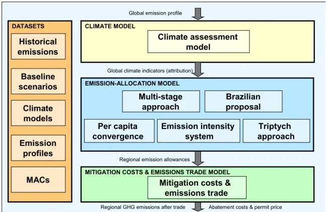
The FAIR 2.0 model consists of three sub-models as outlined below − a simple climate model, an emission allocation model and a mitigation costs and emissions trade model (Figure 2.1):

1. The climate model calculates the greenhouse gas concentrations, radiative forcing of GHGs and other reactive gases (aerosols), global temperature increase, rate of

temperature increase, as well as the sea-level rise for the global emission scenarios and GHG emission profiles associated with different levels of GHG concentration

stabilisation targets. A special climate attribution submodel calculates the regional contribution to global temperature increase and other climate indicators on the basis of the effect of their historical emissions.

2. The emission allocation model calculates regional emission allowances for ten future commitment approaches, divided into five groups:

a. The Multi-Stage approach: a top-down approach3 with a gradual increase in the number of countries involved and their level of commitment according to participation and differentiation rules, such as per capita income or per capita emissions (Berk and den Elzen, 2001). A more simplified Multi-stage approach is included here too, with fewer stages and policy variables, and with threshold levels based on the so-called Capability-Responsibility index (den Elzen et al., 2003a). b. The Brazilian Proposal approach: a top-down approach allocating emission

reductions on the basis of contribution to global temperature increase combined with an income threshold for participation for the non-Annex I regions (den Elzen et al., 1999).

c. Convergence approaches: top-down approaches in which emission allowances are calculated on the basis of convergence rules. Four types of convergence regimes are included:

(i) ‘Contraction & Convergence’, or Per Capita Convergence, i.e. emission allowance convergence towards equal per capita emissions (Meyer, 2000); (ii) CSE convergence: the Contraction & Convergence approach with basic

sustainable emission rights, as introduced by the Centre of Science and Environment (CSE) (CSE, 1998);

(iii) Preference Score approach: a combination of the grandfathering entitlement method and a per capita convergence approach (Bartsch and Müller, 2000). (iv) Multi-criteria convergence: distribution of commitments based on different

weighting of criteria (population, GDP and emissions).

d. Emission intensity system approaches: the emission intensity of the economy is the emissions per unit of economic activity expressed in Gross Domestic Product (GDP). Three types of emission intensity systems are included:

(i) Emission Intensity Convergence approach: a top-down approach with convergence of emission intensities;

(ii) Emission Intensity Targets approach: a bottom-up approach4, in which all regions adopt GHG intensity targets right after 2012 when achieving an income threshold.

3_{A top-down approach first defines the global GHG emission profile (budget) and then allocates the emission}

allowances or reductions.

(18)

(iii) Jacoby Rule approach: a bottom-up approach, in which both participation and emission reductions depend on the per capita income (Jacoby et al., 1999). This approach can also be applied top-down by scaling total emissions in the direction of the emission profile.

e. Triptych approach: a sector and technology-oriented bottom-up approach in which overall emission allowances are determined by applying various differentiation rules to different sectors (e.g. convergence of per capita emissions in the domestic sector, efficiency and de-carbonisation targets in the industrial and the power generation sector) (Blok et al., 1997; Phylipsen et al., 1998).

3. The mitigation costs and emissions trade model calculates the tradable emission permits, the international permit price and the total abatement costs, with or without emission trading, according to the regional emission allowances of a certain climate regime. The model makes use of Marginal Abatement Cost curves (MACs)5 used to derive permit supply and demand curves under different regulation schemes in any emissions trading market using the same methodology as Ellerman and Decaux (1998).

Historical emissions Baseline scenarios Climate models MACs

Regional GHG emissions after trade Abatement costs & permit price Mitigation costs &

emissions trade

MITIGATION COSTS & EMISSIONS TRADE MODEL

Climate assessment model

Global climate indicators (attribution)

CLIMATE MODEL

Global emission profile

Regional emission allowances Per capita convergence Multi-stage approach Emission intensity system EMISSION-ALLOCATION MODEL Brazilian proposal Triptych approach DATASETS Emission profiles

Figure 2.1. Schematic diagram of FAIR 2.0 showing its framework and linkages.

2.2 New elements of FAIR 2.0

Since 2001, the FAIR 1.0 model (den Elzen et al., 2001) has undergone numerous major and minor modifications, with several new elements being introduced, leading to the present FAIR 2.0 model. These new elements are briefly summarised here:

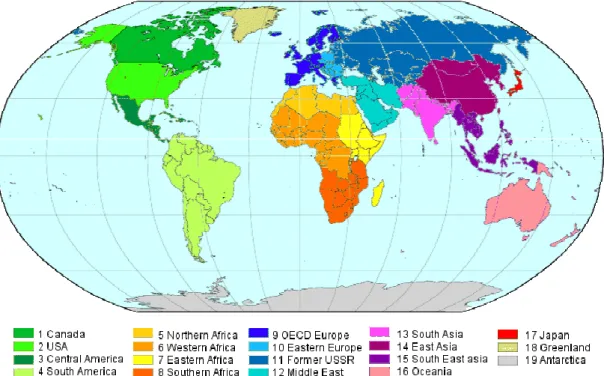
1. An increase in the number of world regions – from 13 to 17 – in line with the IMAGE 2.2 world regions. These are Canada, USA, Central America, South America, Northern Africa, Western Africa, Eastern Africa, Southern Africa, OECD Europe, Eastern Europe, Former USSR (FSU), Middle East, South Asia (including India), East Asia (including China), South East Asia, Oceania and Japan (see Figure 2.2).

5_{A marginal abatement curve (MAC), differing per country, reflects the additional costs of reducing the last}

(19)

2. All emission allocation and cost calculations now at the level of CO2-equivalent

emissions instead of (fossil) CO2-only.6

3. Historical emission datasets now based on the latest EDGAR-HYDE 1.4 historical emissions database (all GHGs and other reactive gases), with the energy and industry-related CO2emissions, and the land-use-related CO2 emissions, based on the latest

CDIAC-ORNL database.

4. The set of baseline emission scenarios updated with the new IMAGE 2.2 IPCC SRES emission scenarios (IMAGE-team, 2001), along with the original IPCC SRES scenarios (Nakicenovic et al., 2000). The recently developed Common POLES-IMAGE (CPI) emission scenario is also included.

5. Inclusion of new IMAGE 2.2 emission profiles, stabilising the atmospheric CO2

-equivalent concentrations7 at different levels (550, 650 and 750 ppmv) (Eickhout et al., 2003).

6. Replacement of the climate model by the stand-alone IMAGE 2.2.version of the Atmosphere-Ocean System (AOS). For alternative climate calculations, the climate model also includes alternative simple carbon-cycle and climate models of the UNFCCC, along with the Impulse Response Functions (IRFs) based on simulation experiments with nine general circulation and other climate models.

7. Improvement of the climate ‘attribution’ module for calculating the regional

contributions to global climate indicators using the recent UNFCCC methodology.8

8. An updated Triptych approach methodology, including all GHG emissions, as well as improvements to the convergence regime. New climate regimes like Global

Compromise, Jacoby rule and different emission intensity systems are also included. 9. Extension of the Multi-Stage regime with a new participation threshold based on both

per capita income and per capita emissions, called the Capability-Responsibility (CR) index (den Elzen et al., 2003a). Other new elements include: (i) accounting for a policy delay between passing thresholds and taking action; (ii) using a reference period for calculating threshold levels and (iii) making income-dependent GHG intensity improvements in stage 2.

10. The new mitigation costs and emissions trade model used to analyse the economic implications of a future commitment regime under different emission trading markets. 11. The possibility of evaluating the Kyoto Protocol and its flexibility; the implementation

of US intensity targets.

6_{Similar to the Kyoto Protocol (KP), the GHG emissions targets are calculated as CO}

2-equivalent emissions,

i.e. the sum of the Global Warming Potential (GWP)-weighted emissions of six specified GHG emissions or groups of gases covered in the Kyoto Protocol. These are carbon dioxide (CO2), methane (CH4), nitrous oxide

(N2O), hydrofluorocarbons (HFCs), perfluorocarbons (PFCs) and sulphur hexafluoride (SF6). 7_CO

2-equivalent concentration is a measure of the contribution of the various GHGs to the radiative forcing

in any given year in terms of CO2. 8_{http://unfccc.int/program/mis/brazil/}

(20)

(21)

3 Datasets of FAIR 2.0

3.1 Historical emissions data

The historical emission datasets cover the greenhouse gases, CO2, CH4, N2O and the

halocarbons (only those covered by the Kyoto Protocol) for the period from 1760 to 1995 and are mainly used by the climate model. The emissions are based on the CDIAC-ORNL database (Andres et al., 1998; Marland et al., 1999) and EDGAR 1.4 (Emission Database for Global Atmospheric Research) database (Olivier and Berdowski, 2001; Van Aardenne et al., 2001). The CDIAC-ORNL database includes the CO2 emissions from fossil fuel

combustion and cement production for 1751-1995 on country level, and the regional CO2 emissions from land-use changes, based on Houghton (1999). The EDGAR 1.4

database includes historical emissions of the greenhouse gases, CO2, CH4, N2O, the

halocarbons and F-gasses from fossil fuel combustion9, industrial and agricultural sources, and emissions from biomass burning and deforestation for 1890-1995. The historical emissions of all gases included occur at the level of IMAGE 2.2 regional aggregation of 17 world regions (see Figure 2.2).10

Table 3.1. The different historical emission datasets included

Historical emission datasets

• CDIAC (energy, industrial & CO2 land-use emissions)

• EDGAR/HYDE (GHG emissions: energy, industry & land use and agriculture)

3.2 Baseline scenarios

The baseline scenarios are used for future (1995-2100) projections of population, Gross Domestic Product (GDP) (in US$ or PPP$)11 and baseline emissions of GHGs (without climate policy). Different types of baseline scenarios are included (see Table 3.2). The IMAGE 2.2 IPCC SRES emission scenarios are extensively described in IMAGE-team (2001) and the original IPCC SRES scenarios in Nakicenovic et al. (2000).12 The common POLES-IMAGE (CPI) emission scenario (see den Elzen et al. (2003a)) is largely based on the existing POLES reference scenario up to 2030 (Criqui and Kouvaritakis, (2000) and extended to 2100 by using the IMAGE 2.2 model (IMAGE-team, 2001).

Table 3.2. The different baseline scenarios included

Baseline scenarios

• Six IMAGE 2.2 IPCC SRES emission scenarios • Six original IPCC SRES emission scenarios • Common IMAGE-POLES (CPI) emission scenario

9_{The bunker CO}

2 emissions can be treated as a separate region, but may also be included in the regional

emissions.

10_{To this end, only the regional CO}

2 emissions from the Houghton land-use changes had to disaggregate at

the level of our IMAGE 2.2 regions using historical population data.

11_{The Purchase Power Parity (PPP) is an alternative indicator for GDP per capita, based on relative}

purchasing power of individuals in various regions, i.e. the value of a dollar in any country, or, in other words, the dollars needed to buy a set of goods compared to the amount needed to buy the same set of goods in the United States.

12_{We used the detailed regional information of our own IMAGE 2.2 implementation of the IPCC SRES}

emissions scenarios (IMAGE-team, 2001) for disaggregating the regional emissions of the IPCC SRES scenarios at the level of the IMAGE 2.2 regions.

(22)

3.3 Emission profiles

The emission profiles describe emission pathways up to 2100, and even to 2300, leading to a stabilisation of the CO2-equivalent concentrations13 at different levels. The FAIR 2.0

model includes the IMAGE 2.2- and IPCC-SAR emission profiles (Table 3.3). The IMAGE 2.2 GHG emission profiles result in a stabilisation of the CO2-equivalent

concentrations at 550, 650 and 750 ppmv in 2100, 2150 and 2150, respectively (S550e, S650e and S750e profiles), (Eickhout et al., 2003). The corresponding CO2 emission

profiles result more-or-less in a stabilisation of the respective CO2 concentrations of 450,

550 and 650 ppmv for S450c, S550c and S650c profiles. The range in the temperature increase associated with these two profiles will depend on the uncertainty attached to the ‘climate sensitivity’ parameter. The S550e profile may result in a maximum global mean temperature increase of less than 2°C, with a low to medium level of climate sensitivity, defined as the equilibrium global mean surface-temperature increase resulting from a doubling of CO2-equivalent concentrations. The IPCC estimates the range of the climate

sensitivity between 1.5 and 4.5°C, with a median value of 2.5°C (sensitivities near the median are much more likely than sensitivities near the outer ends). The S650e profile only remains below this level if the climate sensitivity level is low. Consequently, this profile is unlikely to meet the EU target. For the S750e profile this is even more unlikely. In the case of a serious climate sensitivity, the EU target will not be met under all three profiles. The IPCC-SAR CO2-only emission profiles are the CO2 emission profiles based on inverse

calculations (e.g. Enting et al. (1994)) with the Bern carbon cycle model of Joos et al. (1996; 1999) using the delayed response concentration stabilisation profiles of Wigley et al. as input (Wigley et al., 1996). The corresponding CO2-only emission profiles stabilise the

CO2 concentrations at 450 and 550 ppmv (WRE S450c and WRE S550c profile).

Users can also construct their own CO2-only emission profile, which can be combined with

the non-CO2 emissions from the IMAGE 2.2 emission profiles to create a multi-gas profile.

This profile can then be evaluated with respect to its climate impacts and can be used in the emission allocation model.

Up to 2012 all emission profiles incorporate the implementation of the Annex I Kyoto Protocol targets, an optimal level of banking excess emissions by the Former Soviet Union (FSU) and Eastern Europe and adoption of the proposed greenhouse gas intensity target for the USA (-18% between 2002-2012) (van Vuuren et al., 2002; White-House, 2002a).

Table 3.3. The different emission profiles included

Emission profiles

• Three IMAGE 2.2 GHG emission profiles, resulting in stabilisation of the CO2-equivalent

concentration at 550, 650 and 750 ppmv (S550e, S650e and S750e profiles). • Three IMAGE 2.2 CO2-only emission profiles, resulting in stabilisation of the CO2

concentration at 450, 550 and 650 ppmv (S450c, S550c and S650c profiles). • Two IPCC-SAR CO2-only emission profiles, resulting in stabilisation of the CO2

concentration at 450 and 550 ppmv (WRE S450c and WRE S550c profiles). • User-owned defined CO2-only emission profile.

13_CO

2-equivalent concentration is a measure of the contribution of the various GHGs to the radiative forcing

(23)

3.4 Climate models

Table 3.4 lists the climate models included in the FAIR model. The IMAGE-AOS climate model is used for the default global climate calculations. For alternative calculations, either the UNFCCC-ACCC climate model, or eight alternative climate models based on Impulse Response Functions (IRFs) (as explained in Box 1 in Chapter 4) can be used. The IRFs are calculated on the basis of simulation experiments with various Atmosphere-Ocean General Circulation Models (AOGCMs).

Table 3.4. The different climate models included

Climate models

• IMAGE-AOS climate model • UNFCCC-ACCC climate model

• Eight alternative climate models based on IRFs (Table 4.4).

3.5 Marginal Abatement Cost (MAC) curves

This section starts with a brief introduction to Marginal Abatement cost (MAC) curves explaining what MAC curves are and what they represent. How are MAC curves constructed from the macro-economic model WorldScan and the energy system model TIMER and how are they calculated in more bottom-up studies?

3.5.1 What are Marginal Abatement Cost (MAC) curves?

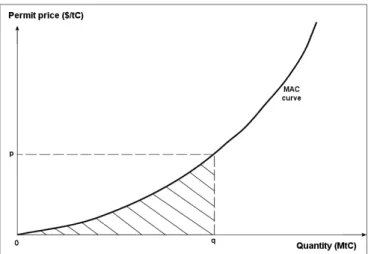
A MAC curve reflects the additional costs of reducing the last unit of carbon and is

upward-sloping: i.e. marginal costs rise with the increase of the abatement effort. Figure 3.1 shows a stylised Marginal Abatement Cost curve. The point (q,p) on the curve represents the marginal cost, p, of abating an additional unit of carbon emissions at quantity q. The surface under the curve (hatched area) represents the total abatement costs of carbon emission reduction q. In this way the MAC curves, representing the costs and potential of emission reductions for the different regions, gases and sources, are used by the emission trading and abatement costs models and (see Chapter 6)14.

Figure 3.1. Marginal Abatement Cost Curve. The hatched area indicates the total cost of abatement under emission reduction objective q.

14_{One great advantage of using MAC curves is that they clearly show the effects of permit trading. However,}

there are also some limitations: carbon leakage cannot be taken into account, and while total abatement costs are reflected by MACs, welfare losses are not (see section 6.2).

(24)

3.5.2 How are MAC curves constructed?

Macro-economic and energy system models are used as examples for constructing MAC curves for CO2 energy-relatedemissions, for which a carbon tax on fossil fuels is imposed

to induce emission abatements. Such a tax is differentiated according to the CO2 emissions

(the carbon content) from the fuels. In response, emissions will decrease as a result of such measures as fuel switching (e.g. from coal to gas), decreases in energy consumption and the introduction of zero-carbon energy options (renewables and nuclear). The carbon tax can be seen as an indicator of the marginal abatement costs. MAC curves can be created by

plotting different tax levels against the corresponding emission reductions i.e.: 1. Working with a reference projection (baseline) in which the carbon tax is zero.

2. Calculating by successive simulations, the emission reduction levels (q) associated with the carbon tax (p) through successive simulations that change from level to level. 3. Developing the MAC curve as illustrated in Figure 3.1 on the basis of the points (q,p). Opposite to the above described top-down method, MAC curves can also be constructed through a bottom-up approach. In a bottom-up approach, the MAC curves are constructed according to detailed abatement options per gas and source. The different options are sorted according to their relative costs and plotted against their reduction potential. The fitted line then forms the MAC curve. To use the MAC curves for the different baseline scenarios of the various models, we have to express the MACs as percentile reductions with respect to the baseline emissions. Absolute MAC curves can be created by projecting the relative MAC curves on to the baseline emissions used in the FAIR model.

3.5.3 The different MAC curves in the FAIR model

Table 3.5 shows the different sets of MAC curves included in the FAIR model, with the models and background of the MAC curves explained below. The final MAC curves, as implemented in the FAIR model, are described in more detail in Appendix A.

Table 3.5. The different sets of MAC curves in the FAIR model

• CO2 MAC curves (energy- and industry-related CO2 emissions) from the energy

system models, TIMER and POLES, and the macro-economic model, WorldScan. • CO2 sequestration MAC curves from the IMAGE 2.2 model.

• Non-CO2 MAC curves from the GECS project and EMF 21.

CO2 MAC curves of WorldScan

WorldScan is a multi-sector, multi-region applied general equilibrium model15 (CPB, 1999). The model is developed for exploring long-term economic scenarios, with a focus on long-term growth and trade in the world economy based on neo-classical theories of growth and trade. The model can produce carbon shadow prices for any constraint on carbon emissions, but also the other way around, producing emission reductions compared to the baseline levels for any shadow price. The MAC curves of WorldScan do not change significantly with time. The reason for this is that the model does not include carbon-tax induced technological developments (learning) or limitations in time delays of

implementing the options. Effects that can be of influence over time include structural economic changes, however, their impact seems.

(25)

CO2 MAC curves of TIMER

The TIMER (Targets Image Energy Regional model) model aims to analyse the long-term dynamics of the energy system, particularly with regard to energy conservation and the transition to non-fossil fuels. It also calculates energy-related greenhouse gas emissions (de Vries et al., 2002; van Vuuren and de Vries, 2001). An important aspect of the model is the modelling of technological development in terms of log-linear learning curves

according to which the efficiency of processes improves with accumulated output

(‘learning-by-doing’). These processes are price-induced energy efficiency improvements, fossil fuel production, non-fossil-based electricity and biofuels (van Vuuren and de Vries, 2001). Use of learning curves implies a path-dependent potential for technological change. Another important aspect is the limitations set on capital turnover. The fact that capital depreciation is limited within the model by its average lifetime introduces inertia between the signal (carbon price or tax) and the responses mentioned, which is crucial for the MAC curves. Both the learning effect and the delays make the actual MAC curve for each region dependent on earlier abatement action.

CO2 MAC curves of POLES

POLES (Prospective Outlook on Long term Energy Systems) is a worldwide sectoral energy model that simulates energy demand and supply on a year-to-year basis up to 2030 (Criqui et al., 1999). The model includes 38 countries or regions and 15 main energy demand equations for each country, 24 power generation technologies, of which 12 new and renewable technologies are explicitly incorporated. The POLES model also projects the energy sector’s CO2 emissions up to 2030, as well as the marginal abatement cost curves

for these emissions in each of the 38 countries or regions. Inertia and technological learning similar to TIMER are modelled in POLES.

CO2-sequestration MAC curves of IMAGE 2.2

The CO2-sequestration MAC curves describe the potential and costs of carbon

sequestration from afforestation activities. Population growth, technological development of the agricultural sector and the production of food and feed determines the amount of land in each region required to feed the world population, to fulfil the demand for timber and to grow modern biofuels. Land that is no longer required can be used for other purposes like sink sequestration. The IMAGE 2.2 model (IMAGE-team, 2001) is used to determine the area of land that will become available in a certain baseline period and how much carbon can be potentially sequestered in that area. The Surplus Potential Productivity (SPP) of the plantation is calculated to take into account the amount of carbon that would be sequestered by the re-growing vegetation of abandonment agricultural land. The SPP represents the net C sequestration by the plantation minus that of the original vegetation. The carbon

plantations are assumed to be implemented in areas that have no other use during a 50-year period given the baseline. The SPP information for each 0.5 x 0.5 degree grid cell is

aggregated to the level of the 17 regions, while the annual C sequestration is calculated as a mean during a 50-year period. The carbon supply curves form the basis of the sink MAC curves by taking into account the cost of land, and the forest establishment and the operation and maintenance costs. The differences in prices of land between regions result from differences in land and soil quality. The settlement costs are taken from the IPCC (1996a) and the operation and maintenance costs estimated as a standard value of $25 per hectare for OECD Europe and a variable value for the other regions on the basis of per capita incomes. The potential sink area is reduced by a factor representing political, social

(26)

and economic obstacles. These barriers cause a reduction in the area through an

implementation degree of 10% in 2010 and 30% in 2030 and onwards, so that the actual potential is only this percentage of the full potential.

Non-CO2 MAC curves from the GECS project

The GECS project (Greenhouse gas Emission Control Strategies) (Criqui, 2002) is a European multi-partner project in the DG Research 5th Framework Program. The project was implemented to enhance the European capabilities for the economic analyses of long-term (2030) multi-gas abatement strategies in the perspective of future climate negotiations. The non-CO2 MACs developed in this project have been constructed mostly on the basis of

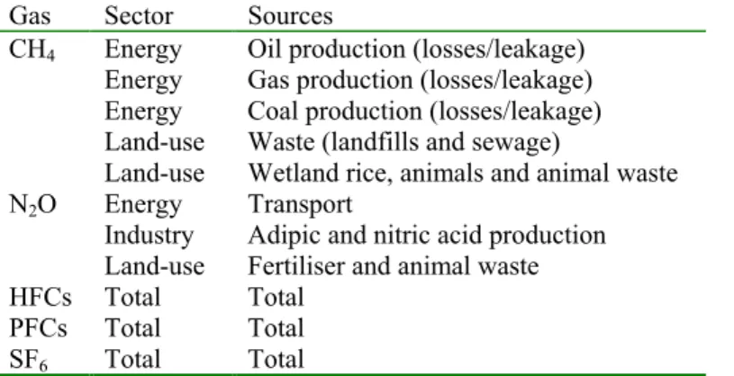
detailed abatement options per gas and per source (bottom-up). Eleven different sources for three different sectors for five non-CO2 GHGs are distinguished per region (see Table 3.6). Table 3.6. Sectoral non-CO2 MAC curves from the GECS project

Gas Sector Sources

CH4 Energy Oil production (losses/leakage)

Energy Gas production (losses/leakage) Energy Coal production (losses/leakage) Land-use Waste (landfills and sewage)

Land-use Wetland rice, animals and animal waste N2O Energy Transport

Industry Adipic and nitric acid production Land-use Fertiliser and animal waste

HFCs Total Total

PFCs Total Total

SF6 Total Total

Non-CO2 MAC curves from EMF 21

The non-CO2 MAC curves from EMF 21 are also constructed on the basis of detailed

abatement options per gas and per source. Eight different sources for the five non-CO2

GHGs are distinguished per region (see Table 3.7). The HFCs, PFCs and SF6 are

considered as one group (F gases) for which one MAC curve is available. The list of abatement options is compiled from analyses for the USA (USEPA, 1999; USEPA, 2001a; USEPA, 2001b), the EU (EC, 2000; EC, 2001) and the ICF (2002). Expert knowledge of the region is used to omit options from individual regions on a case-by-case basis. Each abatement option is characterised in terms of its costs and benefits. The costs include capital and maintenance costs, while the benefits include the value of methane, either as natural gas or electricity, the non-GHG benefits of the abatement option and the value of abating the GHG.

Table 3.7. Sectoral non-CO2 MAC curves from EMF 21

Gas Sector Sources

CH4 Energy Oil production (losses/leakage)

Energy Gas production (losses/leakage) Energy Coal production (losses/leakage) Land-use Manure management

Land-use Landfills

N2O Industry Adipic acid production

Industry Nitric acid production F gases Total HFCs, PFCs and SF6

(27)

4 Simple climate model

The climate model of FAIR 2.0 consists of a global climate submodel (1) and a climate attribution submodel (2).

1. The global climate submodel calculates the greenhouse gas concentrations, temperature increase, rate of temperature increase and sea-level rise for the global emissions

scenarios and emission profiles. It also evaluates the indicators using climate targets (see Table 4.1).

2. The climate attribution submodel calculates the regional contributions to different climate change indicators (CO2 (-equivalent) concentrations, cumulative emissions,

radiative forcing, temperature increase and sea-level rise).

The IMAGE-AOS climate model calculates the default global climate. For alternative calculations, either the UNFCCC-ACCC climate model or alternative climate models based on the IRFs derived from simulation experiments with various Atmosphere-Ocean General Circulation Models (AOGCMs) can be used (den Elzen et al., 2002). These models, along with the climate attribution model, will be briefly described below; more details can be found in Appendixes B and C.

Table 4.1. Main climate targets formulated by the European Commission and the Dutch Ministry of Housing, Spatial Planning and the Environment (VROM)

EU _{• Global-mean surface temperature increase relative to pre-industrial levels} less than 2.0 o_{C in the long-term}

Dutch ministry: _{• Global-mean surface temperature increase relative to pre-industrial levels} are less than 2.0 o_{C in the long term.}

• Rate of global temperature increase less than 0.1 o_{C per decade}

• Global-mean sea level rise less than 50 cm in the long term

4.1 IMAGE-AOS climate model

IMAGE 2.2 Atmosphere Oceanic System (IMAGE-AOS) consists of an oceanic carbon, atmospheric chemistry and climate model (Eickhout et al., 2002). The atmospheric CO2

concentration is calculated using a mass balance equation, with a carbon flux between the atmosphere (and natural vegetation (NEP16) as exogenous input, based on data from scenario runs with IMAGE 2.2 (IMAGE-team, 2001). This includes changes in terrestrial uptake resulting from global warming and changes in ambient CO2 concentration, as well

as anthropogenic land use and land cover changes. The oceanic uptake is calculated using the oceanic carbon model, IMAGE 2.2 (Eickhout et al., 2002), i.e. the box-diffusion type model from Joos et al. (1996; 1999); for more details see Appendix B). The atmospheric chemistry model calculates the concentration of the non-CO2 GHGs using single fixed

lifetimes for the atmospheric decay of non-CO2 gases, except for CH4, HCFCs and HFCs.

For the lifetime of these gases, dependencies on the concentration of the OH radical are included in the methodology on the basis of the IPCC-TAR (Third Assessment Report) methodology of Prather et al. (2001). The default climate model is formed from the

Upwelling-Diffusion Climate Model (UDCM) on the basis of the MAGICC model (Hulme et al., 2000; Raper et al., 2001). The main parameters of the IMAGE-AOS climate model are presented in Table 4.2.

16_{NEP - Net Ecosystem Productivity}

(28)

Table 4.2. Main parameters* of the IMAGE-AOS climate model as implemented in the FAIR 2.0 model

Model parameters Central value

• Forcing a doubling of CO2 concentration (in W/m2)

• Climate sensitivity parameter, i.e. equilibrium global-mean surface temperature increase resulting from a doubling of CO2-equivalent concentrations (in o_C)

• Vertical diffusivity between ocean layers (in cm2_/sec)

• Upwelling rate at initial steady state (in m/yr)

• Temperature change ratio from polar to non-polar region (-) • Depth of ocean mixed layer (in m)

• Depth of other ocean layers (in m)

5.325 2.5 2.30 4 0.2 60 100

* See Appendix B for other detailed parameters of IMAGE-AOS.

4.2 UNFCCC-ACCC climate model

One alternative model configuration is specified according to the Terms of Reference of the UNFCCC project entitled ‘Assessment of Contributions to Climate Change’ (UNFCCC-ACCC).17 Here, Impulse Response Functions (IRFs) (see Box 1) based on convolution integrals for concentrations, temperature change and sea-level rise are used. There are four four-term CO2 IRFs included for calculating the CO2 concentration. Three IRFs are based

on three different parameterisations18_{of the Bern Carbon Cycle model in Joos et al. (1996)}

as applied in the IPCC-TAR (Third Assessment Report), and one IRF on the Bern Carbon Cycle model, as applied in the IPCC-SAR (Second Assessment Report) (Table B.1). The change in concentration of the non-CO2 GHGs (CH4, N2O, HFCs, PFCs, and SF6) is

defined by a single-fixed lifetime expression (Table B.2). For both temperature change and sea-level rise, two-term IRFs were fit to data from a 900-year long experiment using the HadCM3 Coupled General Circulation climate Model (CGCM) (Table B.3).

Table 4.3. Main parameters of the UNFCCC climate model as implemented in the FAIR 2.0 model

• Climate sensitivity parameter, i.e. equilibrium global-mean surface temperature increase resulting from a doubling of the CO2 equivalent concentrations

• Four IRFs from the Bern Carbon Cycle model (Bern-TAR, Bern-SAR low, Bern-SAR standard, Bern-SAR high) (see Table B.1)

4.3 Alternative climate models

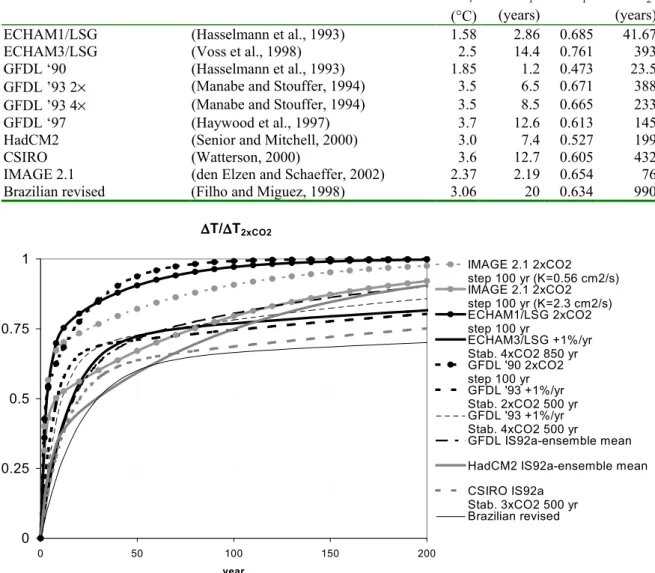
The alternative climate models are based on temperature change IRFs derived from a range of eight AOGCM experiments. Table 4.4 describes the eight IRFs on the basis of AOGCM experiments, i.e.: ECHAM1/LSG (Hasselmann et al., 1993), ECHAM3/LSG (Voss et al., 1998), GFDL ’90 (Hasselmann et al., 1993), GFDL ’93 2× and GFDL ’93 4× (Manabe and Stouffer, 1994), GFDL ’97 (Haywood et al., 1997), HadCM2 (Senior and Mitchell, 2000) and CSIRO (Watterson, 2000), as described in den Elzen and Schaeffer (2002). Two other IRFs, based on the IMAGE 2.1 climate model and the Brazilian revised climate model, are also included (Filho and Miguez, 1998). Figure 4.2 shows the response of the IRFs to a

17_{See the UNFCCC website: http://unfccc.int/issues/ccc.html.} 18_{Different parameterisations of the CO}

(29)

sudden doubling of CO2 concentration.19 Also indicated in Figure 4.2 is the ‘outlier’

response of the IRFs used in the revised Brazilian Proposal (Filho and Miguez, 1998).

19_{Due to the scenario dependence of IRF fits mentioned above, the IRF responses to this sudden doubling of}

CO2 resemble only the ‘original’ climate model response to such forcing when the same, extreme, scenario

was used when determining IRF parameters.

Box 1. What is an Impulse Response Function (IRF)?

IRFs form a simple tool for mathematically describing (‘mimic’) transient climate model response to external forcing. A two-term IRF model used here (as in Hasselmann et al. , 1993) is based on the following convolution integral, relating temperature response ∆T to time-dependent external forcing Q(t):

' ) / 1 ( ) ' ( ) ( 0 2 1 / )' ( 2 2 _Q _t _l _e _dt Q T t T t t s t t s s s

ò

_êëé

å

_úûù ∆ = ∆ = − − × × _τ τ _(4.1)

where Q2_× is the radiative forcing for a doubling CO2 and ls the amplitude of the 1st or 2nd

component with exponential adjustment time constant, τs, while l₁ + l₂ =1. ∆T2×/Q2× equals

the climate sensitivity parameter λ (Cess et al., 1989). In an alternative formulation, we can define C=1/λ, and characterise C as the effective heat capacity of the climate system, including climate-response feedback. An example of IRF performance is seen in Figure 4.1 where results from the CSIRO GCM experiment (Watterson, 2000) and the IRF model are shown using appropriate parameter values. Both models were forced with the same

scenario, i.e. the radiative forcing following the IS92a scenario, starting with the historical pathway from 1881 and stabilising at 3 × the present CO2 concentration (den Elzen and

Schaeffer, 2002). -1 0 1 2 3 4 5 1880 1980 2080 2180 2280 2380 year ∆∆∆∆ T ( K )

Figure 4.1. The IRF model (heavy line) attuned to the CSIRO GCM data (light line) (Watterson, 2000).

(30)

Table 4.4. Parameters for temperature change Impulse Response Functions derived from a range of AOGCM experiments (den Elzen and Schaeffer, 2002)

Climate model Reference T_eq

(°C) T 1 τ (years) T a₁ T 2 τ (years)

ECHAM1/LSG (Hasselmann et al., 1993) 1.58 2.86 0.685 41.67

ECHAM3/LSG (Voss et al., 1998) 2.5 14.4 0.761 393

GFDL ‘90 (Hasselmann et al., 1993) 1.85 1.2 0.473 23.5

GFDL ’93 2× (Manabe and Stouffer, 1994) 3.5 6.5 0.671 388

GFDL ’93 4_× (Manabe and Stouffer, 1994) 3.5 8.5 0.665 233

GFDL ‘97 (Haywood et al., 1997) 3.7 12.6 0.613 145

HadCM2 (Senior and Mitchell, 2000) 3.0 7.4 0.527 199

CSIRO (Watterson, 2000) 3.6 12.7 0.605 432

IMAGE 2.1 (den Elzen and Schaeffer, 2002) 2.37 2.19 0.654 76

Brazilian revised (Filho and Miguez, 1998) 3.06 20 0.634 990

∆∆∆∆T/∆∆∆∆T2xCO2 0 0.25 0.5 0.75 1 0 50 100 150 200 year IMAGE 2.1 2xCO2 step 100 yr (K=0.56 cm2/s) IMAGE 2.1 2xCO2 step 100 yr (K=2.3 cm2/s) ECHAM1/LSG 2xCO2 step 100 yr ECHAM3/LSG +1%/yr Stab. 4xCO2 850 yr GFDL '90 2xCO2 step 100 yr GFDL '93 +1%/yr Stab. 2xCO2 500 yr GFDL '93 +1%/yr Stab. 4xCO2 500 yr GFDL IS92a-ensemble mean HadCM2 IS92a-ensemble mean CSIRO IS92a Stab. 3xCO2 500 yr

Brazilian revised

Figure 4.2. The temperature response (normalised by climate sensitivity) to a sudden doubling of the atmospheric CO2 concentration at time t=0 for the various IRFs in Table 4.4 (den Elzen and Schaeffer, 2002).

4.4 Climate attribution submodel

UNFCCC-ACCC and alternative climate models

Contributions of emission regions to climate change indicators like greenhouse gas

concentration, radiative forcing, temperature change and sea-level rise are calculated for the UNFCCC-ACCC climate model and the alternative climate models. This is done by

separately applying all equations defined at global level to the emissions of the individual emitting regions.20 Linearity of the equations ensures correct global totals.21

20_{The climate attribution model is extensively described in den Elzen et al. (2002).}

21_{Only the relationship between concentration and radiative forcing in the UNFCCC-ACCC climate model is}

non-linear (‘saturation effect’).Due to the saturation effect, the radiative forcing of each additional unit of concentration from the ’early emitters‘ (low saturation of CO2 absorption) is larger than the radiative forcing

of an additional unit from the ’later emitters‘ (higher saturation of CO2 absorption). Therefore attributing the

(31)

Thus, in this approach the global carbon cycle is divided into R hypothetical independent carbon pools, or isolated boxes, one for each emitting region, described by the same C-cycle model and parameters. The global total is simply the linear addition of contributions by all isolated region boxes. We will term this the ‘linear approach’ of concentration attribution. Concentrations and removal rates for region r in this approach depend only on (anthropogenic) emission (history) of this one region, not on emissions of other regions. In reality, there is only one global carbon cycle.

IMAGE-AOS

The following alternative attribution calculation as applied to the IMAGE-AOS climate attribution model of regional attribution to global CO2 concentrations appreciates this.

) ( ) ( ) ( ) (t C ₂ Er ₂ t r t t CO CO r _ρ _τ ρ& = ⋅ − (4.2)

with τ(t) as a time-depending global single ‘effective’ lifetime, or fairly instantaneous turnover time, of the excess CO2 mass in the atmosphere. Removal rate in each ‘region pool’

now depends on global carbon-cycle dynamics, including non-linearity induced by emissions from all regions. An advantage of this method is that global concentrations can be calculated using any (non-linear) carbon-cycle model, like the model in IMAGE-AOS. Non-linearity in the carbon cycle are potentially important. For example, Enting and Law (2002a) showed atmospheric lifetime of CO2 to increase with higher CO2 concentration; this can be accounted

for using the alternative attribution approach. Here, we will use the IMAGE-AOS model, which, in contrast to the UNFCCC-ACCC carbon cycle model, includes saturation of the CO2-fertilisation effect over the whole historical and scenario time period. Since

IMAGE-AOS further includes scenario-dependant land use changes, it has direct anthropogenic influence on the terrestrial carbon cycle, whereas the UNFCCC-ACCC carbon cycle model represents, in a sense, the natural ‘undisturbed’ carbon cycle. The effects of using the alternative (‘non-linear’ approach, as described above) to attribute concentrations, and the effect of using a carbon cycle including these non-linearity, is analysed in den Elzen et al. (2002). The methodology of calculating the contributions of emission regions to temperature change and sea level rise within the IMAGE-AOS climate model are described in Appendix C, and is based on earlier work of den Elzen and Schaeffer (den Elzen et al., 1999; den Elzen and Schaeffer, 2002; den Elzen et al., 2002).

Table 4.5. The main parameters of the climate attribution model as implemented in the FAIR 2.0 model

• Starting date of historical emissions (1765-1990) • Ending date of future emissions (1990-2300)

• Evaluation date of attribution calculations (2000-2300) • Historical land use emissions (CDIAC or IMAGE-AOS)

• Coverage of GHG emissions (only fossil CO2 emissions, all anthropogenic

CO2 emissions and all anthropogenic GHG emissions)

• Inclusion or exclusion of non-linearity in the attribution of CO2 concentration and

(32)

Box 3. Modelling the attribution of non-linearity in radiative forcing

Calculating regional contributions to global radiative forcing by a greenhouse gas is now more complicated due to the non-linearity in radiative forcing than contributions to concentration increases and temperature change and sea level rise. There are two

possibilities for calculating radiative forcing (Qg in W⋅m-2_{) : (i) in proportion to attributed}

concentrations of a greenhouse gas (the so-called proportional method) or (ii) in proportion to the changes in attributed concentrations (see Appendix C). The first methodology

ignores the partial saturation effect and considers equal radiative effects of the ‘early’ and ‘late emitters’, whereas the second includes this partial saturation effect, implying a larger radiative effect of the ‘early emitters’ (Annex I regions). For UNFCC-ACCC, and the IMAGE-AOS climate attribution model, the proportional method (i.e. partitioning the forcing) occurs in the default calculations in proportion to the instantaneous partitioning of the concentrations used, as specified in ACCC-TOR and Appendix C.

Box 4. Modelling the emissions time frame

An important element in the ACCC-TOR methodology is the time frame of the attribution calculations. Variations are possible in the length of the period over which historical emissions are taken into account. In addition, contributions can be calculated for an

evaluation date some time after the emission end date, so that future, or delayed, effects are included, as well as the different atmospheric decay rates of the various GHGs. In this way, the climate indicator is ‘backward looking’ (i.e. takes historical emissions into account), ‘backward discounting’ (early emissions weigh less depending on the decay in the

atmosphere) and ‘forward looking’ (i.e. takes future effects of the emissions into account) (e.g., Höhne and Harnisch (2002)). This leads to the following three policy choices: (1) a horizon of historical emissions or emission starting date, (2) a horizon of future emissions, or emission end date and (3) evaluation date of attribution calculations.

(33)

5 Emission allocation model

The emission allocation model aims at calculating regional emission allowances or

assigned amounts (we prefer to call it emission allowances) for various climate regimes for the differentiation of future commitments. The following climate regimes are implemented in the model:

1. Brazilian Proposal (BP) 2. Multi-Stage approach (MS)22 3. Per Capita Convergence (PCC) 4. CSE Convergence (CSE) 5. Preference Score approach (PS) 6. Multi-Criteria Convergence (MCC) 7. Emission Intensity Convergence (EIC) 8. Emission Intensity Targets approach (EIT) 9. Jacoby rule approach (JR)

10. Triptych approach (TT).

The following sections comprise short overviews of each regime (or approach), along with the relevant methodology. Before presenting the overviews, however, we will first briefly outline the equity principles and other dimensions of possible regimes for the

differentiation of future commitments, with the aim of positioning the various regimes (see Table 5.1).

5.1 Equity principles and other dimensions

Equity principles – Equity principles refer to more general notions or concepts of distributive justice or fairness. Many different categorisations of equity principles can be found in the literature e.g. Ringius et al. (1998; 2002) and, when not contradictory, cannot in general be easily reformulated. To date, a number of key equity principles that have been explored or invoked in the international climate can be identified:

- Egalitarian: i.e. all human beings have equal rights in the ‘use’ of the atmosphere. - Sovereignty and acquired rights: all countries have a right to use the atmosphere,

and current emissions constitute a ‘status quo right’.

- Responsibility / polluter pays: the greater the contribution to the problem, the greater the share of the user in the mitigation / economic burden.

- Capability: the greater the capacity to act or ability to pay, the greater the share in the mitigation / economic burden.

The basic needs/no-harm principles are included here as a special expression of the capability principle: the least capable regions should be exempted from the obligation to share in the emission reduction effort so as to secure their basic needs. For a more detailed description please refer to Berk et al. (2002b) and den Elzen et al. (2003b).

The Per Capita Convergence, Multi-Criteria Convergence, CSE Convergence and

Preference Score approaches are ultimately based on a combination of the egalitarian and sovereignty principles, while leaving aside the principle of responsibility. The Brazilian Proposal and Jacoby rule are clearly oriented to the responsibility and capability principles, respectively. The Emission Intensity Targets approach is based mainly on capability. However, please note that it is more oriented towards opportunity for mitigation than economic capability. The Multi-Stage approaches (including SMS) are based on a

(34)

combination of the responsibility and capability principles, but may also include elements related to the egalitarian principle, for example, by using per capita emissions levels as the burden-sharing key. The Triptych approach is based mainly on the capability to act, but also encompasses elements of the egalitarian equity principle.

Other dimensions - In addition to equity principles, there are a number of other dimensions of possible regimes for the differentiation of future commitments, e.g. Berk et al. (2002b).

Problem definition (burden-sharing or resource-sharing. The climate change problem can be

defined either as a pollution problem or as a property-sharing issue. These different

approaches have implications for the design of climate regimes. In the first approach, burden sharing will focus on defining who should reduce or limit pollution and by how much. In the latter approach the focus is on who has what user rights; the reduction of emissions will be in line with the user rights.

Emission limit. One can define the emission reduction top-down by first defining globally

allowed emissions and then applying certain participation and differentiation rules for allocating the overall reduction effort needed. Bottom-up emission reduction is defined by allocating emission control efforts among Parties without a predefined overall emission reduction effort. In the top-down approach, the question of adequacy of commitments is separated from the issue of burden differentiation. In the bottom-up approach, the two are dealt with at the same time.

Participation (thresholds/ timing). Another dimension is the degree of participation: who

should participate in sharing the burden and when? This issue concerns discussions on both the types of thresholds for participation and the threshold level or the timing. At the same time, there is no need for all Parties to participate in the same way.

Type of commitment. The approaches for differentiation of commitments can either

pre-define the allocations of emissions over time or make the allocation dependent on actual developments in levels of economic activity, population or emissions. In an ex ante analysis this results in baseline-dependent allowance schemes. The level of dependency on actual developments can vary from low, as in the Per Capita Convergence approach (dependent on population only), to high, as in the Multi-Stage approach (dependent on population, income and emissions).

Form of commitment. The form of the commitment may be the same for all countries, such as

the binding emission target in the Kyoto Protocol, but may also be defined in a differentiated manner (see e.g. Baumert et al., (1999); Claussen et al., (1998); Philibert and Pershing (2001)). Instead of being fixed absolute targets, commitments may be defined as relative or dynamic targets, such as reduction in energy and/or carbon intensity levels, or in terms of policies and measures. There is also the option of non-binding commitments. In addition, the legal nature of the commitment can be either binding or voluntary.23

Scope of the commitment. This dimension is related to the question of whether the

commitment covers all GHGs and sectors or is limited to particular GHGs or sectors.

Particularly for developing countries, new commitments could be limited to particular sectors

23_{Formally, commitments are always voluntary in the sense that countries voluntarily commit themselves to}

international agreements. However, a country is formally bound to meet its obligations once ratified. In the case of voluntary commitments there is no formal obligation to achieve a material result (e.g. reduction in emissions).