Compiling biodiversity accounts with the GLOBIO model

(1)

Compiling biodiversity accounts

with the GLOBIO model

A case study of Mexico

Note

Aafke Schipper, Marlon Tillmanns, Paul Giesen, Stefan van der Esch 01 March 2017

(2)

Colophon

Compiling biodiversity accounts with the GLOBIO model: a case study of Mexico PBL Netherlands Environmental Assessment Agency

The Hague, 2017

PBL publication number: 2607 Corresponding author

Aafke.Schipper@pbl.nl Authors

Aafke Schipper, Marlon Tillmanns, Paul Giesen, Stefan van der Esch with contributions from

Raúl Figueroa Díaz, José Luis Ornelas-de Anda (National Institute of Statistics and Geography (INEGI), Aguascalientes City, Mexico)

Parts of this publication may be reproduced, providing the source is stated, in the form: PBL Netherlands Environmental Assessment Agency, title and year of publication.

PBL Netherlands Environmental Assessment Agency is the national institute for strategic policy analysis in the field of environment, nature and spatial planning. We contribute to improving the quality of political and administrative decision-making by conducting outlook studies, analyses and evaluations in which an integrated approach is considered paramount. Policy relevance is the prime concern in all our studies. We conduct solicited and unsolicited research that is both independent and scientifically sound.

(3)

Although ecosystems and biodiversity are highly important to mankind, their value is not yet included in national accounts. The United Nations Statistics Division (UNSD) developed a conceptual method to establish ecosystem accounts (Experimental Ecosystem Accounting or EEA) as part of the System of Environmental Economic Accounts (SEEA). However, concrete guidelines are lacking and actual experiences with national ecosystem accounting are very limited. In the present study, we aimed to evaluate the applicability of the GLOBIO modelling approach (version 3.5) to establish biodiversity accounts. The GLOBIO model is designed to assess past, present and future human-induced changes in terrestrial biodiversity at regional to global scales. GLOBIO is built upon a set of quantitative relationships that describe biodiversity responses to anthropogenic pressures. In GLOBIO 3.5, biodiversity responses are quantified as the mean species abundance (MSA), which expresses the mean abundance of original species in disturbed conditions relative to their abundance in undisturbed habitat, as an indicator of the degree to which an ecosystem is intact.

To test the applicability of the GLOBIO modelling approach for accounting purposes, we compiled biodiversity accounts for the country of Mexico, which is known for its high biodiversity and high quality of geographical data. We quantified the accounts based on two indicators: ecosystem extent, quantified as the total area of each ecosystem type within the country, and ecosystem condition, quantified as the area-weighted MSA per ecosystem type, as function of both land use and infrastructure. We compiled and compared the accounts based on three different land-use maps. The first map was a 0.5° by 0.5° raster land-use map for the year 2010, as produced by the GLOBIO model (version 3.5). In this map land use is represented as the fractions of the different land use type present per grid cell. The other two were vector-based maps (i.e., each polygon representing a single land-use type) that included, respectively, 19 aggregated and 178 detailed land-use types specific to Mexico. These maps were provided by Mexico’s National Statistical and Geographical Institute (INEGI) and represented the years 2011-2013.

The accounts showed that either shrubland or forest comprised the most abundant ecosystem type in Mexico, depending on the land-use map used. Overall MSA values were 0.65, 0.72 and 0.75 for the detailed vector-based, aggregated vector-based and GLOBIO land-use maps, respectively. These differences were mainly due to differences in the land-use classifications and allocation of MSA values to land-use types. For example, the detailed vector-based map included considerable amounts of secondary vegetation (i.e., relatively low MSA value), whereas the aggregated map and the GLOBIO land-use map did not distinguish this land-use type. Infrastructure impacts were subordinate and highly similar between the three maps.

Based on the case study results we conclude that the MSA values and cause-effect relationships from the GLOBIO model provide a transparent, flexible and relatively time- and cost-efficient approach to compile national biodiversity accounts. Further, we found clear trade-offs between the generic global-scale land-use map from the GLOBIO model and the country-specific vector-based maps. Compiling accounts vector-based on the GLOBIO land-use map ensures compatibility with the MSA cause-effect relationships in GLOBIO and enhances comparability among countries. Yet, the coarse resolution and model uncertainties in the land-use allocation module in the current version of GLOBIO raise questions as to the representativeness of this map in an accounting context. The country-specific land-use maps were much more detailed, which is a clear advantage at least for compiling extent accounts. Moreover, using country-specific land-use data may stimulate stakeholder engagement and hence legitimacy and uptake of the results in decision-making. However, the MSA-based biodiversity accounts require an MSA value to be

(5)

assigned to each ecosystem unit or land-use type, which may require additional data and analysis. Moreover, as land-use classifications may differ (slightly) among countries, the use of country-specific land-use maps may reduce comparability of the accounts among countries. Given the trade-offs among the different land-use maps, it might be worth using and comparing multiple land-use input maps when compiling national ecosystem accounts, including a generic, global-scale land-use (or land cover) map as well as more detailed country-specific maps. In addition, further experimental ecosystem accounting may benefit from incorporating other biodiversity metrics that are complementary to MSA. For example, species-habitat indices (SHIs) quantify (changes in) the amount of suitable habitats of single species by combining land cover or land-use maps with literature- and expert-based judgment on the occurrence ranges and habitat preferences of single species. Thus, SHIs could be used in addition to MSA in order to account for differences in species pools among countries.

(6)

1 Introduction

Ecosystems are providing various goods and services that contribute to human existence or wellbeing (Costanza et al., 1997). Examples include the provisioning of drinking water and timber, sequestration of carbon, and pollination of food crops (MA, 2005). The worldwide degradation of ecosystems and biodiversity and the increasing recognition of their values have prompted increasing calls for better protection and more systematic consideration of ‘natural capital’ in decision making (CBD, 2010). In particular, there have been frequent calls to better integrate ecosystem values into national accounting systems (Obst et al., 2016). The System of Environmental Economic Accounts – Experimental Ecosystem Accounting (SEEA-EEA) was developed as a general framework to achieve this (United Nations, 2014). The aim of ecosystem accounting is to quantify (changes in) ecosystem assets (i.e., stocks) and services (i.e., flows) in a way that is aligned with the approaches prescribed for economic accounting (Edens and Hein, 2013; United Nations, 2014).

In general, the accounting model proposes to measure the (changes in) ecosystem assets by considering the extent and condition of given ecosystem functional units (see Table 1.1 for the corresponding definitions). Extent and condition are quantified based on, respectively, area indicators and characteristics pertaining to for example water, soil, carbon, vegetation or biodiversity (United Nations, 2014; De Jong et al., 2015). The extent and condition of a given ecosystem functional unit determine its capacity to deliver certain ecosystem services, which in turn contribute to so-called ecosystem benefits (i.e., the part of the service that is actually being used). These benefits can be quantified either in biophysical terms (for example, the amount of carbon emissions sequestered per year) or in monetary values (for example, the amount of fish supplied to the market expressed in terms of the market price). Finally, the assets, services and benefits provided by the ecosystem functional units can be aggregated and reported over so-called accounting units. Accounting units combine multiple ecosystem functional units into larger units based on administrative boundaries, with the country level typically representing the highest level of aggregation (United Nations, 2014)

Despite the launch of the SEEA-EEA framework and the increasing interest in ecosystem accounting, there is only limited practical experience, and there remain various challenges in the integration of measures of ecosystem assets and services into the standard national accounts. Apart from the challenges involved in the monetary valuation of ecosystems (Obst et al., 2016), the quantification of the biophysical stocks and flows is not straightforward either, as this requires clear definitions of concepts, system boundaries, and measures of stock and flow that can be quantified and aggregated in a way that is meaningful in an accounting context (Edens and Hein, 2013; Schröter et al., 2014; United Nations, 2014). One particular challenge is involved in including biodiversity in ecosystem condition accounts. Although the species diversity of an ecosystem is highly relevant for both its functioning and its resilience (Hooper et al., 2005; Hooper et al., 2012), accounting for species diversity is complex and experiences with biodiversity accounting are much less advanced than with for example water or carbon accounting (UNEP-WCMC, 2015).

In the present study, we compiled biodiversity accounts for the country of Mexico, which is known for its high diversity of ecosystems and endemic species (González-Abraham et al., 2015). We had the following specific aims:

1) to test the applicability of the GLOBIO modelling approach for establishing biodiversity accounts, by combining maps of biodiversity pressures with cause-effect relationships expressing corresponding impacts on biodiversity;

(7)

2) to compare biodiversity accounts based on ecosystem functional units established at different levels of detail.

To compile the biodiversity accounts, we used two indicators. First, we quantified the extent of different ecosystem functional types, which is considered the foundation of a biodiversity account in the broadest sense as it provides information on ecosystem diversity (UNEP-WCMC, 2015). Second, we quantified biodiversity as function two anthropogenic pressures that are generally considered to have high impacts on terrestrial biodiversity, namely land use and infrastructure (Benítez-López et al., 2010; Newbold et al., 2015). To that end, we used the Mean Species Abundance (MSA) indicator and underlying cause-effect relationships from the GLOBIO model (Alkemade et al., 2009; PBL, 2016). The MSA indicator represents the mean abundance of original species in the current situation compared to their mean abundance in an undisturbed reference situation. It ranges between 0 and 1, where 1 indicates that there is no difference in mean abundance between the current and undisturbed state of the ecosystem. As MSA includes an inherent baseline (i.e., the undisturbed reference situation) and is easily aggregated across scales (PBL, 2016), it has high potential for ecosystem accounting purposes (UNEP-WCMC, 2015). Moreover, as MSA can be quantified based on easily retrievable pressure data and existing cause-effect relationships, the approach had the potential to be readily applied to any country.

Table 1.1 Explanation of terms used in ecosystem accounting, based on the SEEA-EEA framework description (United Nations, 2014).

Term Description

Ecosystem functional unit A spatial unit containing a combination of biotic and abiotic components and other characteristics that function together. Conceptually similar to the definition of an ecosystem as ‘a dynamic complex of plant, animal and micro-organism communities and their non-living environment interacting as a functional unit’, as used by the Convention on Biological Diversity.

Ecosystem type Broad categorization of ecosystems made for accounting purposes (e.g., forest, grassland, shrubland, wetland).

Ecosystem accounting unit A relatively stable (mostly administrative) area relevant for analysis and

reporting purposes.

Ecosystem asset A spatial area containing a combination of biotic and abiotic components and other characteristics that function together (note that this is in fact similar to an ecosystem functional unit). Ecosystem assets are described in terms of extent, condition (which may include biodiversity) and services.

Ecosystem extent The total area of a given ecosystem type within a given ecosystem accounting unit.

Ecosystem condition The overall quality of an ecosystem asset.

Ecosystem service The contribution of the ecosystem asset to benefits used in economic and other human activities.

(8)

2 Methods

2.1 Ecosystem functional units

We used land-use maps as basis to distinguish ecosystem functional units. In order to evaluate the sensitivity of the biodiversity accounts to the level of (spatial) detail in the underlying ecosystem units, we established and compared accounts based on three land-use maps:  A land-use map from the GLOBIO model, version 3.5 (PBL, 2016). In GLOBIO, land-use maps

are compiled from the GLC2000 map combined with regional land-use data from the IMAGE model. GLC2000 which is a global land cover map with a resolution of 30 arc seconds (about 1 km at the equator) including 23 different land cover classes. To include information on anthropogenic land use, the GLC2000 map is combined with land-use data from the IMAGE model, resulting in a 0.5o_{by 0.5}o_{land-use map with the fraction of each unique combination} of land cover and use type per grid cell (PBL, 2016). For the present study, we used a GLOBIO land-use map for the year 2010, using land-use input data and assumptions in accordance with the baseline scenario as used in the fourth Global Biodiversity Outlook (PBL, 2014). For Mexico, this map includes 36 distinct combinations of a given GLC2000 land cover class and land-use type/intensity (see Table S1 in the Supplementary Material).

 A vector-based land-use map provided by Mexico’s National Institute of Statistics and Geography (INEGI). This map is based on data from the period 2011 – 2013 and includes two hierarchic thematic classifications: 19 aggregated land-use types (Table S2) and 178 detailed classes (see Table S3).

2.2 Quantifying ecosystem extent

To quantify ecosystem extent based on the fractional GLOBIO land-use map, we used the fractions of each land-use type per grid cell multiplied with the land surface area (km2_{) of the} corresponding cell. We aggregated this per land-use type over the cells, resulting in the total area per land-use type. To quantify ecosystem extent based on the detailed land-use maps (vector), we first reprojected the maps into Mexican Albers Equal-Area Conic projection (centered on Mexico), using ArcGIS (10.3.1, ESRI 2015). We then calculated the area of each polygon using the “Calculate Geometry” function and used the “Summary Statistics” function to sum the polygon areas per land-use type.

2.3 Quantifying biodiversity

We quantified the biodiversity of each ecosystem functional unit by quantifying MSA in relation to two pressures, i.e., land use and infrastructure. We did this for each pressure separately as well as the two pressures combined.

2.3.1 MSA in relation to land use

To quantify MSA in relation to land use, we used the land-use type specific MSA values as included in the GLOBIO model (version 3.5) (PBL, 2016). These MSALU values have been quantified based on a meta-analysis of literature studies that reported on the abundance of

(9)

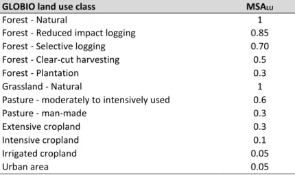
species in a given land-use type and intensity in comparison to their abundance in an undisturbed reference situation (Alkemade et al., 2009; PBL, 2016). The GLOBIO land-use map of Mexico consisted of 36 unique combinations of land-cover and land use (Table S1), corresponding with 12 GLOBIO LU classes and corresponding MSA values (Table 2.1).

Table 2.1 The GLOBIO land-use classes occurring in Mexico, with corresponding

MSALU values.

GLOBIO land use class MSALU

Forest - Natural 1

Forest - Reduced impact logging 0.85 Forest - Selective logging 0.70 Forest - Clear-cut harvesting 0.5

Forest - Plantation 0.3

Grassland - Natural 1

Pasture - moderately to intensively used 0.6

Pasture - man-made 0.3

Extensive cropland 0.3

Intensive cropland 0.1

Irrigated cropland 0.05

Urban area 0.05

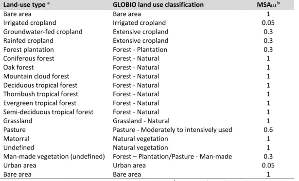
For the vector maps, we quantify MSA in relation to land use by assigning an MSALU value to each land-use type. For the aggregated land-use types (Table 2.2), we made the following assumptions:

 We interpreted rainfed agriculture (agricultura de temporal) and groundwater-fed agriculture (agriculture de humedad) as extensive cropland (MSA = 0.3), under the assumption that the absence of irrigation is indicative of extensive use.

 We interpreted cultivated grassland (pastizal cultivado) as original grasslands used for livestock grazing (MSA = 0.6).

 We assumed that undefined vegetation (especial - otros tipos) is in natural, undisturbed state (MSA = 1)

 We interpreted man-made vegetation (vegetación inducida) as plantation, using the MSA value for both forest plantation and man-made pasture (MSA = 0.3).

For the detailed land-use types (Table 2.3), the following assumptions were made:

 We interpreted cultivated forest (bosque cultivado), man-made forest (bosque inducido) and palm plantation (palmar inducido) as forest plantation (MSA = 0.3), because they are dominated by introduced tree species (INEGI, 2015).

 We interpreted cultivated grassland (pastizal cultivado) as original grasslands used for livestock grazing (MSA = 0.6) and man-made grassland (pastizal inducido) as man-made pasture (MSA = 0.3), where succession back to natural forest vegetation is prevented due to intensive use (including grazing) (INEGI, 2015).

 The MSA value of secondary vegetation is strongly dependent on the succession stage (age) of the vegetation (Newbold et al., 2015; PBL, 2016). However, because we could not retrieve the age of the secondary vegetation from the classification, we assigned a general MSA value of 0.5 to all secondary vegetation (Alkemade et al., 2009).

(10)

Table 2.2 Reclassification of the aggregated land-use types into GLOBIO land-use

classes with corresponding MSALU values.

Land-use type a _{GLOBIO land use classification} _MSA LU b

Bare area Bare area 1

Irrigated cropland Irrigated cropland 0.05 Groundwater-fed cropland Extensive cropland 0.3 Rainfed cropland Extensive cropland 0.3 Forest plantation Forest - Plantation 0.3 Coniferous forest Forest - Natural 1

Oak forest Forest - Natural 1

Mountain cloud forest Forest - Natural 1 Deciduous tropical forest Forest - Natural 1 Thornbush tropical forest Forest - Natural 1 Evergreen tropical forest Forest - Natural 1 Semi-deciduous tropical forest Forest - Natural 1

Grassland Grassland - Natural 1

Pasture Pasture - Moderately to intensively used 0.6

Matorral Natural vegetation 1

Undefined Natural vegetation 1

Man-made vegetation (undefined) Forest – Plantation/Pasture - Man-made 0.3

Urban area Urban area 0.05

Bare area Bare area 1

a_{The original Spanish name can be found in Table S2.}b_{See PBL (2016)}

Table 2.3 Reclassification of the detailed land-use types into GLOBIO land-use

classes with corresponding MSALU values.

Land-use type a _{GLOBIO land use classification}b _MSA LU

BA, BB, BG, BJ, BM, BP, BPQ, BQ, BQP, BS, SAP, SAQ, SBC, SBK, SBP, SBQ, SBQP, SBS, SG, SMC, SMQ, SMS, VPN

Forest – Natural 1

BC, BI, VPI Forest – Plantation 0.3

PH, PN, PY, VH, VS, VSI, VW Grassland - Natural 1 PC Pasture – Moderately to intensively used 0.6

PI Pasture – Man-made 0.3

MC, MDM, MDR, MET, MK, MKE, MKX, ML, MRC, MSC, MSCC, MSN, MST, PT, VA, VD, VG, VHH, VM, VT, VU

Natural vegetation 1

VSA, VSa, VSh (including all subtypes) Secondary vegetation 0.5 RA, RAP, RAS, RP, RS, RSP, Irrigated cropland 0.05 HA, HAP, HAS, HP, HS, HSP, TA, TAP, TAS,

TP, TS, TSP

Extensive cropland 0.3

AH, ZU Urban area 0.05

ADV, DV Bare area 1

a_{The full names (Spanish) can be found in Table S3.}

2.3.2 MSA in relation to infrastructure

To quantify MSA in relation to infrastructure disturbance, we used the approach as implemented in the GLOBIO model. In GLOBIO, a 1 km disturbance zone is delineated along the road network, which is assigned an MSA value of 0.78 (PBL, 2016). The road network is retrieved from the Global Road Inventory Project (GRIP) database, which contains georeferenced vector data on

(11)

five road types (highways, primary roads, secondary roads, tertiary roads and local roads) for 222 countries worldwide (Meijer et al., in prep.).

In GLOBIO, the potential infrastructure disturbance (i.e., without accounting for any other impacts on biodiversity) is calculated based on the proportion of each 0.5o_{by 0.5}o_{grid cell that} is within the infrastructure impact zone, as

if ( 𝐴𝐼,𝐶

𝐴𝐶 ≥1, 𝑀𝑆𝐴𝐶,𝐼 = 0.78, 𝑀𝑆𝐴𝐶,𝐼 = 1 − (

𝐴𝐼,𝐶

𝐴𝐶 ∙ 0.22) ) (Eq.1)

where AI,C is the area of the infrastructure disturbance zone in grid cell C, AC is the area of that grid cell, and MSAC,I is the potential impact of infrastructure in cell C. Thus, this equation states that if the area of the infrastructure impact zone is equal or larger than the area of the grid cell, the maximum potential impact of infrastructure is obtained for that cell, and the cell gets an MSAI value of 0.78. If the area of the infrastructure impact zone is smaller than the area of the grid cell, the maximum possible loss of biodiversity (0.22) will be reduced based on the fraction of the land use type that is within the infrastructure impact zone. In the impact calculation, it is assumed that infrastructure impacts are lower in protected areas as compared to unprotected areas, because of targeted spatial planning and regulation measures. Therefore, in protected areas the MSAI value of 0.78 is replaced by MSAI = 0.90.

To quantify the potential impact of infrastructure (MSAI) for the discrete vector-based land use maps, a buffer of 1 km was created along each side of the roads, which was assigned an MSAI value of 0.78. The areas outside the buffer zone were assigned an MSAI value of 1 (i.e., no infrastructure impact).

2.3.3 MSA in relation to both land use and infrastructure

To quantify the combined impacts of land use and infrastructure, we followed the GLOBIO model approach. In GLOBIO, it is assumed that the direct land use impacts of agriculture and urban areas take precedence over any other impacts, i.e., that there is no further loss of MSA due to other anthropogenic pressures (including infrastructure). In land-use types other than cropland or urban area, impacts of multiple disturbances are assumed to interact probabilistically (response multiplication). Hence,

𝑖𝑓 (𝐿𝑈 = 𝑐𝑟𝑜𝑝𝑙𝑎𝑛𝑑 𝑂𝑅 𝐿𝑈 = 𝑢𝑟𝑏𝑎𝑛,

𝑀𝑆𝐴

𝐶

= 𝑀𝑆𝐴

𝐶,𝐿𝑈

, 𝑀𝑆𝐴

𝐶

= 𝑀𝑆𝐴

𝐶,𝐿𝑈

∙ 𝑀𝑆𝐴

𝐶,𝐼

)

(Eq.2)

where MSAC is the MSA value of cell C due to both land use and infrastructure disturbance, and MSAC,LU and MSAC,I are the MSA values of cell C in relation to land use and infrastructure separately.

Because the GLOBIO land-use map is fractional, the exact locations of the different land-use types in each cell are not known. Therefore, the potential infrastructure impact in each cell is distributed over the land-use types following a predefined order. According to this prioritization, the land-use classes urban area, cropland and pasture get a higher priority than for example natural forest, based on the assumption that roads will be primarily located within urban and agricultural areas. For example, assume that a certain grid cell has a total area of 1000 km2_, consisting of 50 km2_{of urban area, 500 km}2 _{of cropland and 450 km}2 _{of broadleaved deciduous} forest. Assume further that the total area of the infrastructure impact zone is 700 km2_{. According} to the prioritization, the first 50 km2_{of the impacted area is then assigned to urban area, the}

(12)

next 500 km2_{to cropland, and the remaining 150 km}2_{is assigned to broadleaved deciduous} forest. This leaves no direct infrastructure impact for the remaining 300 km2_{of forest area. As it} is assumed that infrastructure causes no (additional) MSA loss in urban areas and cropland, the MSAI value of 0.78 is then assigned only to the 150 km2_{of impacted forest area. This implies} that the 450 km2_{of forest within that grid cell gets an MSAI value of 1- (150/450 ∙ (1-0.78)) =} 0.93.

To calculate the combined impacts of infrastructure and land use based on the vector maps, we used the “Union” function in ArcGIS (10.3.1, ESRI 2015), creating homogenous polygons with respect to both land use and infrastructure impact. The combined MSA per polygon was calculated according to Equation 2, using the “Field calculator” (see Text Box S1 for details). Then we used “Summary statistics” to summarize the MSA values by land-use type.

2.4 Ecosystem types and accounts

For the purposes of national level ecosystem accounting, it is considered appropriate to consider only a limited set of relatively broad ecosystems types comprising commonly understood categories like forests, wetlands, grasslands (United Nations, 2014). For the GLOBIO land use map, we considered five ecosystem types: forest, shrubland or herbaceous vegetation, cropland, pasture and urban area (see Table S1). We merged shrubland and herbaceous vegetation because two of the classes included both types (class 140 and 150). In case of mosaics, we assigned the class to the dominant type.

For the vector-based land use maps, the following assumptions were made to assign each land-use type to an ecosystem type (see Table S2, S3):

 Temporal forest (bosque), rainforest (selva) and plantation (bosque inducido, bosque cultivado) were all assigned to forest.

 Natural grassland/rangelands and pasture (pastizal inducido and pastizal cultivado) were aggregated to grassland.

 The three main secondary vegetation types as distinguished in the detailed land-use map (secondary forest (vegetación secundaria arbôrea; VSA), secondary shrubland (vegetaciôn secundaria arbustiva; VSa) and secondary grassland (vegetaciôn secundaria herbácea; VSh)) were merged with the corresponding primary types.

To create the accounts, the total extent of each ecosystem type was calculated by summing the extents of the constituent land-use types. MSA values were calculated per ecosystem type as area-weighted average over the constituent land-use types.

(13)

3 Results

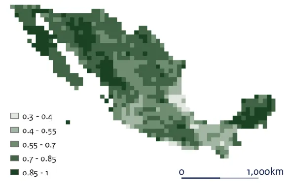
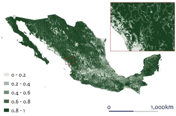
3.1 Spatial patterns in MSA

Overall MSA values showed clear spatial variability across the country (Figure 3.1 – 3.3). For all three land-use maps, relatively high MSA values were found in the north, the north-west (Baja California Peninsula) and north-east (Yucatán Peninsula). Relatively low values were found in the southern part, especially in the region around Mexico City, and along the east coast of the Gulf of California, where cropland and urban area are abundant. In the vector-based map, the road impact zones could be clearly distinguished particularly in areas not affected by land use (Figure 3.2 and 3.3). The spatial patterns as found for the vector-based maps are in agreement with the findings of González-Abraham et al. (2015), who quantified human footprints based on land use, roads and human population density and found high footprint values particularly for the central region surrounding the capital and the eastern coast line along the Gulf of California.

Figure 3.1 MSA in Mexico as function of land use and infrastructure (roads), based on the GLOBIO land-use map.

(14)

Figure 3.2 MSA in Mexico as function of land use and infrastructure (roads), based on the aggregated vector-based land-use map.

Figure 3.3 MSA in Mexico as function of land use and infrastructure (roads), based on the detailed vector-based land-use map.

(15)

3.2 Accounts

3.2.1 Extent

According to the GLOBIO land use map, the largest part of Mexico is covered by forest (Table 3.1), followed by pasture and shrubland/herbaceous vegetation. Forest is also the most extensive ecosystem type according to the aggregated vector-based land-use map, but this map contains more shrubland and cropland and less grassland/pasture than the GLOBIO map (Table 3.2). According to the detailed land-use map, the largest part of Mexico is covered by shrubland (over 40%), followed by forest and cropland (Table 3.3). Differences in ecosystem extents between the two vector-based maps can be explained by the reclassification of the land-use types from the detailed to the aggregated classification. For example, the land-use type “ADV” (“without vegetation”) on the detailed map was classified as “Bare area” in the detailed classification. However, in the aggregated classification, “ADV” is included in “Urban area”. Similarly, the differences in shrubland and forest extent between the aggregated and detailed vector-based maps reflect that some of the detailed shrubland types were reclassified to forest in the aggregated classification.

Urban area constitutes only a small part of the total land surface area, yet it is considerably larger according to the vector-based maps than the GLOBIO map. This might be due to differences in classification as well as explained by the fact that the GLOBIO land-use map is based on the GLC2000 land-cover map. As increases in urban area over time are not accounted for in the GLOBIO land-use allocation module, as is done for cropland and pasture (PBL, 2016), the amount of urban area in the GLOBIO land-use map is fixed at the level as observed in the year 2000.

3.2.2 Condition (biodiversity)

Overall area-weighted MSA values for Mexico as a whole were 0.65, 0.72 and 0.75 for the detailed, aggregated and GLOBIO land-use maps, respectively. Differences were mainly due to differences in land use (MSALU), which in turn reflected differences in classification. For example, classifying “ADV” as bare area yields an MSALU of 1, whereas classifying the same type as urban results in an MSALU of 0.05. The relatively low MSA value for the detailed map in particular mainly reflects the inclusion of secondary vegetation (Table S3), which was not included in the other two maps (Tables S1 and S2). According to the detailed map, a relatively large part of Mexico is covered by secondary vegetation (21.7%), which was assigned a relatively low MSA value of 0.5 (see Table 2.3). Infrastructure impacts were similar across the three maps and considerably lower (i.e., higher MSA) than the land-use impacts.

Table 3.1 Ecosystem accounts based on the GLOBIO land-use map (0.5o_{by 0.5}o_).

Ecosystem type Extent (km2_{) Extent (%) MSA}

LU MSAI MSALU,I

Forest 834,584 33.5 0.96 0.94 0.91 Pasture 544,077 27.9 0.59 0.85 0.51 Shrubland/herbaceous vegetation 346,981 14.9 1.00 0.98 0.98 Cropland 224,988 9.0 0.14 1.00 0.14 Urban area 1,794 0.1 0.05 1.00 0.05 Total 1,952,424 100 0.77 0.93 0.72

(16)

Table 3.2 Ecosystem accounts based on the aggregated vector-based land-use map. MSA values were not calculated for the ecosystem types ‘aquaculture’ and ‘water and wetlands’ because aquatic land-use types are not included in the terrestrial GLOBIO model.

Ecosystem type Extent (km2₎ _{Extent (%)} _MSA

LU MSAI MSA Forest 663,441 34.0 1.00 0.94 0.94 Shrubland 574,399 29.4 1.00 0.94 0.94 Cropland 327,917 16.8 0.22 0.85 0.22 Grassland 248,836 12.7 0.79 0.91 0.72 Plantation 62,872 3.2 0.30 0.89 0.27 Urban area 33,310 1.7 0.05 0.86 0.05 Water and wetlands 26,167 1.3 NA NA NA

Bare area 9,684 0.5 1.00 0.96 0.96

Natural vegetation - undefined 4,605 0.2 1.00 0.91 0.91

Aquaculture 1,069 0.1 NA NA NA

Total 1,952,300 100 0.80 0.92 0.75

Table 3.3 Ecosystem accounts based on the detailed vector-based land-use map. MSA values were not calculated for the ecosystem types ‘aquaculture’ and ‘water and wetlands’ because aquatic land-use types are not included in the terrestrial GLOBIO model.

Ecosystem type Extent (km2₎ _{Extent (%)} _MSA

LU MSAI MSA

Shrubland 792,448 40.6 0.83 0.93 0.77 Forest 467,197 23.9 0.84 0.94 0.79 Cropland 327,917 16.8 0.22 0.85 0.22 Grassland 297,249 15.2 0.68 0.90 0.62 Water and wetlands 37,810 1.9 NA NA NA Urban area 18,537 0.9 0.05 0.78 0.05 Bare area 10,073 0.5 1.00 0.96 0.96

Aquaculture 1,069 0.1 NA NA NA

(17)

4 Discussion

4.1 Biodiversity accounting based on MSA

The aim of this study was to develop and test the GLOBIO modelling approach for developing ecosystem condition accounts based on biodiversity, using the mean species abundance (MSA) indicator. MSA has various properties that make it intrinsically suitable for biodiversity accounting (UNEP-WCMC, 2015):

 It can be mapped to individual ecosystem units, so stocks of biodiversity can be assigned to ecosystem assets.

 It is comparable to a common reference condition indicative of a ‘balanced’ state.

 It can be spatially aggregated to any ecosystem accounting unit, in order to provide an overall indicator of ecosystem condition.

 As long as the input maps on the underlying anthropogenic pressures are the same, the resulting MSA values are comparable over space and time, thus allowing direct comparison of biodiversity stocks in different ecosystem units and among different countries.

To test the applicability of the GLOBIO approach and MSA indicator for biodiversity accounting, we compiled biodiversity accounts for the country of Mexico. To that end, we combined existing cause-effect relationships from GLOBIO (version 3.5) with spatially explicit input data on two main anthropogenic pressures on biodiversity (land use and infrastructure). We used three land-use maps as input: the 0.5° by 0.5° raster-based land land-use map from the GLOBIO model (version 3.5), where land use is represented as fractions of each land-use type per grid cell, and two vector-based maps consisting of, respectively, 19 aggregated and 178 detailed land-use types specific to Mexico, provided by Mexico’s National Institute for Statistics and Geography (INEGI). The vector maps represented the years 2011-2013. As GLOBIO model output is typically produced at decadal intervals, we selected the model year 2010 as closest possible to the date of the vector maps.

Our case study showed that the GLOBIO modelling approach provides a relatively quick, straightforward and transparent method to compile biodiversity accounts. The method is flexible, as it is relatively easily tailored to different input maps of anthropogenic pressures on biodiversity. We further conclude that each of the land-use maps as used in this case study has its pros and cons. The land-use maps that are produced by the GLOBIO model (version 3.5) have the advantage that they are compiled at the global level, which ensures comparability among countries, and that there is a direct link with the MSALU values from the GLOBIO model. Yet, the resolution of the map is rather coarse (0.5° by 0.5°) and the extents of anthropogenic land use (cropland and pasture) result from model simulations rather than observations. In GLOBIO, cropland and pasture ‘claims’ are derived from the IMAGE model, for each of 26 world regions, and then spatially allocated (downscaled) based on land cover (PBL, 2016). As Mexico represents a single world region in the IMAGE model, the cropland and pasture claims are spatially coherent and might therefore be relatively representative. However, for other (smaller) countries, this might be much less so. Further, in the current version of the GLOBIO model, increases in urban area over time are not accounted for, as the level of urbanization is fixed at the value represented in the GLC2000 land cover map (PBL, 2016). This is problematic particularly because urban land-use is expanding rapidly and has a clear impact on biodiversity (Seto et al., 2012; Newbold et al., 2015; Bren d'Amour et al., 2016).

(18)

The country-specific land-use maps available for Mexico contain more spatial detail and are based on observations rather than model simulations. Moreover, using country-specific land-use data may stimulate stakeholder engagement and hence legitimacy and uptake of the results in decision-making (Posner et al., 2016). Yet, the biodiversity accounts retrieved from these land-use maps are contingent on the allocation of MSA values to ecosystem units or land-land-use types. The MSA values as included in the GLOBIO model are retrieved from a global database and global meta-analyses, and the extent to which the values are representative for a specific country (Mexico) has not been tested. For example, assigning a generic MSA value of 0.5 to all secondary vegetation types resulted in a considerably lower overall MSA for the detailed land-use map as compared to the other two maps (Tables 3.1-3.3), whereas it is not known whether the generic value of 0.5 is actually representative. This might be remedied by collecting biodiversity data and defining corresponding MSA values specific to Mexico, but this would go on the expense of reduced comparability among countries.

4.2 Concluding remarks and recommendations

Based on the results obtained, we provide the following conclusions and recommendations:  The MSA values and cause-effect relationships from the GLOBIO model provide a relatively

time- and cost-efficient as well as transparent approach to compile national biodiversity accounts, provided that suitable input data are available regarding the underlying anthropogenic pressures.

 In the present study, we compiled the accounts for a single point in time. However, ultimately, biodiversity accounts should inform about changes in the stock of biodiversity between opening and closing accounting periods (UNEP-WCMC, 2015), i.e., typically from year to year. In principle, the approach presented here is easily applied to multiple subsequent years, provided that the maps of the anthropogenic pressures are updated on a yearly basis. If this is not the case, yearly changes in biodiversity stock might be obtained by dividing the changes observed between two subsequent maps by the duration of the mapping interval.

 Compiling accounts based on the global-scale GLOBIO land-use map ensures compatibility with the MSA cause-effect relationships in GLOBIO and enhances comparability among countries. Yet, the coarse spatial resolution of the map and the model uncertainties in the land-use allocation module in the current GLOBIO model (version 3.5) raise questions as to the representativeness of this map in an accounting context. For accounting purposes, it might be more adequate to rely on monitoring data, but global-scale monitoring data are not available for all land-use types. For example, the state-of-the-art discrete high-resolution (10’’) land cover maps of the Climate Change Initiative provide information on cropland and urban area, but not on use of grasslands (grazing) or forestry. In order to cover these land-use types, remote sensing imagery would need to be integrated with additional data sources on land use.

 In general, country-specific land-use maps are more detailed than global-scale maps, which is a clear advantage at least for compiling extent accounts. However, MSA-based biodiversity accounts require an MSA value to be assigned to each ecosystem unit or land-use type, which may require additional data and analysis. Currently, the MSA values and cause-effect relationships from GLOBIO are derived from a generic database and the extent to which the values are applicable to individual countries has not been evaluated. Moreover, using country-specific land-use maps reduces comparability among countries.

 Given the trade-offs among the different land-use maps, it might be worth using by default multiple maps when compiling national ecosystem accounts, including a generic, global-scale land use (or land cover) map as well as more detailed country-specific maps.

(19)

 Because biodiversity is multi-dimensional, it is generally acknowledged that it cannot be adequately represented by a single indicator or metric (Schipper et al., 2016). Hence, to obtain more inclusive biodiversity accounts, it is worth including additional metrics that are complementary to MSA. For example, species-habitat indices (SHIs) could be used in addition to MSA in order to account for differences in species pools among countries. SHIs quantify (changes in) the amount of suitable habitats of single species by combining land cover or land use maps with literature- and expert-based judgment on the occurrence ranges and habitat preferences of single species (GEO BON, 2015). Like MSA, SHIs are readily spatially aggregated and comparable across space and time.

 In the current study, we focused on ecosystem condition (state) only. Future efforts are needed to quantify also ecosystem services (flows) in the context of ecosystem accounting. Over the recent years, knowledge has greatly improved on the relationships between biodiversity on the one hand and ecosystem functioning and provisioning of services on the other (Isbell et al., 2011; Hooper et al., 2012). However, much of this ecological knowledge is acquired at small scales (e.g. experimental plots) and is still to be incorporated into models of ecosystem services at larger scales.

(20)

References

Alkemade, R., van Oorschot, M., Miles, L., Nellemann, C., Bakkenes, M., ten Brink, B., 2009. GLOBIO3: a framework to investigate options for reducing global terrestrial biodiversity loss. Ecosystems 12, 374-390.

Benítez-López, A., Alkemade, R., Verweij, P.A., 2010. The impacts of roads and other infrastructure on mammal and bird populations: A meta-analysis. Biol. Conserv. 143, 1307-1316.

Bren d'Amour, C., Reitsma, F., Baiocchi, G., Barthel, S., Guneralp, B., Erb, K.-H., Haberl, H., Creutzig, F., Seto, K.C., 2016. Future urban land expansion and implications for global croplands. Proceedings of the National Academy of Sciences of the United States of America.

CBD, 2010. Strategic plan for biodiversity 2011-2020 and the Aichi Targets. Secretariat of the Convention on Biological Diversity, Montreal.

Costanza, R., d'Arge, R., De Groot, R., Farber, S., Grasso, M., Hannon, B., Limburg, K., Naeem, S., Oneill, R.V., Paruelo, J., Raskin, R.G., Sutton, P., vandenBelt, M., 1997. The value of the world's ecosystem services and natural capital. Nature 387, 253-260.

De Jong, R., Edens, B., Van Leeuwen, N., Schenau, S., Remme, R., Hein, L., 2015. Ecosystem Accounting Limburg Province, the Netherlands. Part I: Physical supply and condition accounts. Statistics Netherlands and Wageningen University and Research.

Edens, B., Hein, L., 2013. Towards a consistent approach for ecosystem accounting. Ecol. Econ. 90, 41-52.

GEO BON, 2015. Global Biodiversity Change Indicators. Version 1.2. Group on Earth Observations Biodiversity Observation Network Secretariat, Leipzig.

González-Abraham, C., Ezcurra, E., Garcillán, P.P., Ortega-Rubio, A., Kolb, M., Bezaury Creel, J.E., 2015. The Human Footprint in Mexico: Physical geography and historical legacies. PLoS One 10.

Hooper, D.U., Adair, E.C., Cardinale, B.J., Byrnes, J.E.K., Hungate, B.A., Matulich, K.L., Gonzalez, A., Duffy, J.E., Gamfeldt, L., O'Connor, M.I., 2012. A global synthesis reveals biodiversity loss as a major driver of ecosystem change. Nature 486, 105-U129.

Hooper, D.U., Chapin, F.S., Ewel, J.J., Hector, A., Inchausti, P., Lavorel, S., Lawton, J.H., Lodge, D.M., Loreau, M., Naeem, S., Schmid, B., Setala, H., Symstad, A.J., Vandermeer, J., Wardle, D.A., 2005. Effects of biodiversity on ecosystem functioning: A consensus of current knowledge. Ecological Monographs 75, 3-35.

INEGI, 2015. Guía para la interpretación de cartografía : uso del suelo y vegetación : escala 1:250, 000 : serie V. Instituto Nacional de Estadística y Geografía (INEGI), Aguascalientes (Mexico). Isbell, F., Calcagno, V., Hector, A., Connolly, J., Harpole, W.S., Reich, P.B., Scherer-Lorenzen, M., Schmid, B., Tilman, D., van Ruijven, J., Weigelt, A., Wilsey, B.J., Zavaleta, E.S., Loreau, M., 2011. High plant diversity is needed to maintain ecosystem services. Nature 477, 199-202. MA, 2005. Ecosystems and Human Well-Being: Synthesis report. Millennium Ecosystem

Assessment (MA), Island Press, Washington D.C.

Meijer, J.R., Huijbregts, M.A.J., Schotten, C.G.J., Schipper, A.M., in prep. Mapping the global road network.

Newbold, T., Hudson, L.N., Hill, S.L., Contu, S., Lysenko, I., Senior, R.A., Börger, L., Bennett, D.J., Choimes, A., Collen, B., 2015. Global effects of land use on local terrestrial biodiversity. Nature 520, 45-50.

Obst, C., Hein, L., Edens, B., 2016. National Accounting and the Valuation of Ecosystem Assets and Their Services. Environ. Resour. Econ. 64, 1-23.

Olson, D.M., Dinerstein, E., Wikramanayake, E.D., Burgess, N.D., Powell, G.V.N., Underwood, E.C., D'Amico, J.A., Itoua, I., Strand, H.E., Morrison, J.C., Loucks, C.J., Allnutt, T.F., Ricketts,

(21)

T.H., Kura, Y., Lamoreux, J.F., Wettengel, W.W., Hedao, P., Kassem, K.R., 2001. Terrestrial ecoregions of the worlds: A new map of life on Earth. Bioscience 51, 933-938.

PBL, 2014. How sectors can contribute to sustainable use and biodiversity. CBD Technical Series 79. PBL Netherlands Environmental Assessment Agency, The Hague.

PBL, 2016. The GLOBIO model. A technical description of version 3.5. PBL publication 2369. PBL Netherlands Environmental Assessment Agency, The Hague.

Posner, S.M., McKenzie, E., Ricketts, T.H., 2016. Policy impacts of ecosystem services knowledge. Proceedings of the National Academy of Sciences of the United States of America 113, 1760-1765.

Schipper, A.M., Belmaker, J., Dantas de Miranda, M., Navarro, L.M., Böhning-Gaese, K., Costello, M.J., Dornelas, M., Foppen, R.P.B., Hortal, J., Huijbregts, M.A.J., Martín-López, B., Pettorelli, N., Queiroz, C., Rossberg, A.G., Santini, L., Schiffers, K., Steinmann, Z.J.N., Visconti, P., Rondinini, C., Pereira, H.M., 2016. Contrasting changes in the abundance and diversity of North American bird assemblages from 1971 to 2010. Global Change Biology 22, 3948– 3959.

Schröter, M., Barton, D.N., Remme, R.P., Hein, L., 2014. Accounting for capacity and flow of ecosystem services: A conceptual model and a case study for Telemark, Norway. Ecol. Indic. 36, 539-551.

Seto, K.C., Guneralp, B., Hutyra, L.R., 2012. Global forecasts of urban expansion to 2030 and direct impacts on biodiversity and carbon pools. Proceedings of the National Academy of Sciences of the United States of America 109, 16083-16088.

UNEP-WCMC, 2015. Experimental Biodiversity Accounting as a component of the System of Environmental-Economic Accounting Experimental Ecosystem Accounting (SEEA-EEA). Supporting document to the Advancing the SEEA Experimental Ecosystem Accounting project.

United Nations, 2014. System of Environmental-Economic Accounting 2012 - Experimental Ecosystem Accounting. United Nations, European Commission, Food and Agricultural Organization of the United Nations, International Monetary Fund, Organisation for Economic Co-operation and Development, The World Bank New York.

(22)

SUPPLEMENTARY INFO RM ATION

Table S1 GLOBIO land-use types and classes with corresponding ecosystem types, extent (km2_{) MSA values in Mexico. SL = Selective}

Logging; RIL = Reduced Impact Logging. For a more extensive description of the GLOBIO land-use mapping, see PBL (2016).

Code Land-use type GLOBIO land-use class Ecosystem type Extent (km2₎ _MSA

LU MSAI MSA

10 Tree Cover, broadleaved, evergreen, natural Forest - Natural Forest 157078 1.00 0.97 0.97 11 Tree Cover, broadleaved, evergreen, plantation Forest - Plantation Forest 96 0.30 0.97 0.29 12 Tree Cover, broadleaved, evergreen, harvest Forest - Clear-cut harvesting Forest 10345 0.50 0.97 0.48 13 Tree Cover, broadleaved, evergreen, SL Forest - SL Forest 3509 0.70 0.97 0.68 14 Tree Cover, broadleaved, evergreen, RIL Forest - RIL Forest 668 0.85 0.97 0.82 20 Tree Cover, broadleaved, deciduous, closed, natural Forest - Natural Forest 129312 1.00 0.89 0.89 21 Tree Cover, broadleaved, deciduous, closed, plantation Forest - Plantation Forest 88 0.30 0.88 0.26 22 Tree Cover, broadleaved, deciduous, closed, harvest Forest - Clear-cut harvesting Forest 9485 0.50 0.88 0.44 23 Tree Cover, broadleaved, deciduous, closed, SL Forest - SL Forest 3218 0.70 0.88 0.62 24 Tree Cover, broadleaved, deciduous, closed, RIL Forest - RIL Forest 613 0.85 0.88 0.75 40 Tree Cover, needle-leaved, evergreen, natural Forest - Natural Forest 418234 1.00 0.95 0.95 41 Tree Cover, needle-leaved, evergreen, plantation Forest - Plantation Forest 261 0.30 0.94 0.28 42 Tree Cover, needle-leaved, evergreen, harvest Forest - Clear-cut harvesting Forest 28119 0.50 0.94 0.47 43 Tree Cover, needle-leaved, evergreen, SL Forest - SL Forest 9538 0.70 0.94 0.66 44 Tree Cover, needle-leaved, evergreen, RIL Forest - RIL Forest 1817 0.85 0.94 0.80 60 Tree Cover, mixed leaf type, natural Forest - Natural Forest 56112 1.00 0.94 0.94 61 Tree Cover, mixed leaf type, plantation Forest - Plantation Forest 37 0.30 0.93 0.28 62 Tree Cover, mixed leaf type, harvest Forest - Clear-cut harvesting Forest 4005 0.50 0.93 0.47 63 Tree Cover, mixed leaf type, SL Forest - SL Forest 1358 0.70 0.93 0.65 64 Tree Cover, mixed leaf type, RIL Forest - RIL Forest 259 0.85 0.93 0.79 90 Mosaic tree cover, natural Forest - Natural Forest 398 1.00 0.93 0.93 91 Mosaic tree cover, plantation Forest - Plantation Forest 0.2 0.30 0.93 0.28 92 Mosaic tree cover, harvest Forest - Clear-cut harvesting Forest 25 0.50 0.92 0.46 93 Mosaic tree cover, selective logging Forest - SL Forest 8 0.70 0.92 0.64 94 Mosaic: Tree cover / Other natural vegetation, RIL Forest - RIL Forest 2 0.85 0.92 0.78 110 Shrub cover, closed-open, evergreen Shrubland - Natural Shrubland/Herbaceous 43346 1.00 0.99 0.99 120 Shrub cover, closed-open, deciduous Shrubland - Natural Shrubland/Herbaceous 240289 1.00 0.98 0.98 130 Herbaceous cover, closed-open Herbaceous cover - Natural Shrubland/Herbaceous 29737 1.00 0.95 0.95

(23)

Code Land-use type GLOBIO land-use class Ecosystem type Extent (km2₎ _MSA

LU MSAI MSA

140 Sparse herbaceous or sparse shrub cover Herbaceous cover - Natural Shrubland/Herbaceous 31449 1.00 0.99 0.99 150 Regularly flooded shrub and/or herbaceous cover Herbaceous cover - Natural Shrubland/Herbaceous 2159 1.00 0.97 0.97 160 Cropland, extensive Cropland, extensive Cropland 61312 0.30 1.00 0.30 161 Cropland, irrigated Cropland, irrigated Cropland 53872 0.05 1.00 0.05 162 Cropland, intensive Cropland, intensive Cropland 109803 0.10 1.00 0.10 180 Other natural vegetation Herbaceous cover - Natural Shrubland/Herbaceous 0.6 1.00 1.00 1.00 220 Artificial surfaces and associated areas Urban area Urban 1794 0.05 1.00 0.05

300 Pasturea _Pasture _Pasture ₅₄₄₀₇₇ _0.59 _0.85 _0.51

a_{In GLOBIO, pasture is subdivided into moderately used grassland (MSA = 0.6) and man-made pasture (MSA = 0.3) based on the encompassing biome, following the biome}

classification and map of Olson (2001). If located in a forest biome, the pasture is considered man-made, else it is assumed to be moderately to intensively used grassland (PBL, 2016). The MSA values for pasture as provided in this table comprise area-weighted averages over the two pasture types.

(24)

Table S2 Aggregated land-use types with corresponding GLOBIO land-use classes, ecosystem types and MSA values.

Descriptiona _Translation _{GLOBIO land-use class} _{Ecosystem type} _{Extent (km}2₎ _MSA

LU MSAI MSA

ACUICOLA Aquaculture - Aquaculture 1069 NA NA NA

AGRICULTURA DE HUMEDAD Irrigated cropland Irrigated cropland Cropland 2075 0.05 0.84 0.05 AGRICULTURA DE RIEGO Irrigated cropland Irrigated cropland Cropland 101031 0.05 0.84 0.05 AGRICULTURA DE TEMPORAL Rainfed cropland Extensive cropland Cropland 224810 0.30 0.85 0.30 BOSQUE CULTIVADO Forest plantation Forest - plantation Forest 597 0.30 0.87 0.26 BOSQUE DE CONIFERAS Coniferous forest Forest - natural Forest 168597 1.00 0.93 0.93 BOSQUE DE ENCINO Oak forest Forest - natural Forest 155742 1.00 0.95 0.95 BOSQUE MESOFILO DE MONTANA Mountain cloud forest Forest - natural Forest 18542 1.00 0.93 0.93 ESPECIAL (OTROS TIPOS) Undefined Natural vegetation Natural vegetation -

undefined

4605 1.00 0.91 0.91 MATORRAL XEROFILO Matorral Natural vegetation Shrubland 574399 1.00 0.94 0.94 NO APLICABLE Urban area Urban area Urban area 33310 0.05 0.86 0.05 PASTIZAL Grassland Grassland - natural Grassland 118815 1.00 0.93 0.93 PASTIZAL CULTIVADO Pasture Pasture - moderately to

intensively used

Grassland 130022 0.60 0.89 0.53 SELVA CADUCIFOLIA Deciduous tropical forest Forest - natural Forest 166580 1.00 0.93 0.93 SELVA ESPINOSA Thornbush tropical forest Forest - natural Forest 18865 1.00 0.94 0.94 SELVA PERENNIFOLIA Evergreen tropical forest Forest - natural Forest 91832 1.00 0.95 0.95 SELVA SUBCADUCIFOLIA Semi-deciduous tropical forest Forest - natural Forest 42685 1.00 0.94 0.94 SIN VEGETACION APARENTE Bare area Bare area Bare area 9684 1.00 0.96 0.96 VEGETACION HIDROFILA Water and wetlands - Water and wetlands 26167 NA NA NA VEGETACION INDUCIDA Man-made vegetation

(undefined)

Forest - plantation/man-made pasture

Plantation 62872 0.30 0.89 0.27

(25)

Table S3 Detailed land-use types with corresponding GLOBIO land-use classes, ecosystem types and MSA values.

Code Namea _{GLOBIO land-use class} _{Ecosystem type} _{Extent (km}2₎ _MSA

LU MSAI MSA

ACUI Acuìcola - Aquaculture 1069 NA NA NA

ADV Desprovisto de vegetación Bare area Bare area 388 1.00 0.86 0.86 AH A sentamientos humanos Urban area Urban area 6669 0.05 0.79 0.05

BA Bosque de oyamel Forest - natural Forest 1250 1.00 0.92 0.92

BB Bosque de cedro Forest - natural Forest 21 1.00 0.86 0.86

BC Bosque cultivado Forest - plantation Forest 597 0.30 0.87 0.26

BG Bosque de galeria Forest - natural Forest 204 1.00 0.86 0.86

BI Bosque inducido Forest - plantation Forest 47 0.30 0.82 0.24

BJ Bosque de táscate Forest - natural Forest 1481 1.00 0.92 0.92

BM Bosque mesofilo de montaña Forest - natural Forest 8485 1.00 0.95 0.95

BP Bosque de pino Forest - natural Forest 51664 1.00 0.93 0.93

BPQ Bosque de pino-encino Forest - natural Forest 53679 1.00 0.94 0.94

BQ Bosque de encino Forest - natural Forest 66340 1.00 0.96 0.96

BQP Bosque de encino-pino Forest - natural Forest 29881 1.00 0.95 0.95

BS Bosque de ayarin Forest - natural Forest 244 1.00 0.93 0.93

DV Sin vegetación aparente Bare area Bare area 9684 1.00 0.96 0.96

H2O Cuerpo de agua - Water 14384 NA NA NA

HA Agricultural de humedad anual Extensive cropland Cropland 1324 0.30 0.85 0.30 HAP Agricultural de humedad anual y permanente Extensive cropland Cropland 135 0.30 0.85 0.30 HAS Agricultural de humedad anual y semipermanente Extensive cropland Cropland 278 0.30 0.83 0.30 HP Agricultural de humedad permanente Extensive cropland Cropland 28 0.30 0.81 0.30 HS Agricultural de humedad semipermanente Extensive cropland Cropland 171 0.30 0.85 0.30 HSP Agricultural de humedad semipermanente y permanente Extensive cropland Cropland 140 0.30 0.80 0.30 MC Matorral crasicaule Natural vegetation Shrubland 11504 1.00 0.92 0.92 MDM Matorral desertico micrófilo Natural vegetation Shrubland 190505 1.00 0.93 0.93 MDR Matorral desertico rosetofilo Natural vegetation Shrubland 103862 1.00 0.96 0.96 MET Matorral espinoso tamaulipeco Natural vegetation Shrubland 24813 1.00 0.92 0.92 MK Bosque de mezquite Natural vegetation Shrubland 2346 1.00 0.89 0.89 MKE Mexquital tropical Natural vegetation Shrubland 1253 1.00 0.89 0.89 MKX Mexquital xerofilo Natural vegetation Shrubland 20271 1.00 0.90 0.90

ML Chaparral Natural vegetation Shrubland 20320 1.00 0.96 0.96

(26)

LU MSAI MSA

MSC Matorral sarcocaule Natural vegetation Shrubland 51990 1.00 0.96 0.96 MSCC Matorral sarco-crasicaule Natural vegetation Shrubland 22945 1.00 0.96 0.96 MSM Matorral submontano Natural vegetation Shrubland 23207 1.00 0.94 0.94 MSN Matorral sarco-crasicaule de neblina Natural vegetation Shrubland 5667 1.00 0.94 0.94 MST Matorral subtropical Natural vegetation Shrubland 9783 1.00 0.94 0.94 PC Pastizal cultivado Pasture - moderately to

intensively used

Grassland 130022 0.60 0.89 0.53 PH Pastizal halofilo Natural grassland Grassland 16906 1.00 0.93 0.93 PI Pastizal inducido Pasture - man-made Grassland 60341 0.30 0.89 0.27 PN Pastizal natural Natural grassland Grassland 60625 1.00 0.93 0.93 PT Vegetación de Petén Natural vegetation Water and wetlands 571 1.00 0.98 0.98 PY Pastizal gipsófilo Natural grassland Grassland 389 1.00 0.91 0.91 RA Agricultural de riego anual Irrigated cropland Cropland 53963 0.05 0.85 0.05 RAP Agricultural de riego anual y permanente Irrigated cropland Cropland 9520 0.05 0.85 0.05 RAS Agricultural de riego anual y semipermanente Irrigated cropland Cropland 28350 0.05 0.84 0.05 RP Agricultural de riego permanente Irrigated cropland Cropland 3104 0.05 0.84 0.05 RS Agricultural de riego semipermanente Irrigated cropland Cropland 4329 0.05 0.83 0.05 RSP Agricultural de riego semipermanente y permanente Irrigated cropland Cropland 1764 0.05 0.84 0.05 SAP Selva alta perennifolia Forest - natural Forest 13189 1.00 0.98 0.98 SAQ Selva alta subperennifolia Forest - natural Forest 577 1.00 0.99 0.99 SBC Selva baja caducifolia Forest - natural Forest 62827 1.00 0.94 0.94 SBK Selva baja espinosa caducifolia Forest - natural Forest 2093 1.00 0.92 0.92 SBP Selva baja perennifolia Forest - natural Forest 368 1.00 0.97 0.97 SBQ Selva baja espinosa subperennifolia Forest - natural Forest 4444 1.00 0.99 0.99 SBQP Selva baja subperennifolia Forest - natural Forest 837 1.00 0.99 0.99 SBS Selva baja subcaducifolia Forest - natural Forest 285 1.00 0.95 0.95

SG Selva de galería Forest - natural Forest 43 1.00 0.89 0.89

SMC Selva mediana caducifolia Forest - natural Forest 1352 1.00 0.93 0.93 SMP Selva mediana perennifolia Forest - natural Forest 3 1.00 1.00 1.00 SMQ Selva mediana subperennifolia Forest - natural Forest 14475 1.00 0.97 0.97 SMS Selva mediana subcaducifolia Forest - natural Forest 4080 1.00 0.97 0.97 TA Agricultural de temporal anual Extensive cropland Cropland 175986 0.30 0.86 0.30 TAP Agricultural de temporal anual y permanente Extensive cropland Cropland 15517 0.30 0.84 0.30

(27)

LU MSAI MSA

TAS Agricultural de temporal anual y semipermanente Extensive cropland Cropland 8018 0.30 0.85 0.30 TP Agricultural de temporal permanente Extensive cropland Cropland 14036 0.30 0.85 0.30 TS Agricultural de temporal semipermanente Extensive cropland Cropland 8140 0.30 0.84 0.30 TSP Agricultural de temporal semipermanente y permanente Extensive cropland Cropland 3114 0.30 0.83 0.30 VA Popal Natural vegetation Water and wetlands 1422 1.00 0.96 0.96 VD Vegetación de desiertos arenosos Natural vegetation Shrubland 21386 1.00 0.97 0.97 VG Vegetación ed galería Natural vegetation Shrubland 1501 1.00 0.90 0.90 VH Vegetación halófila xerófila Natural grassland Grassland 23350 1.00 0.93 0.93 VHH Vegetación halófila hidrófila Natural vegetation Water and wetlands 3676 1.00 0.95 0.95 VM Manglar Natural vegetation Water and wetlands 8541 1.00 0.97 0.97

VPI Palmar inducido Forest - Plantation Forest 965 0.30 0.93 0.28

VPN Palmar natural Forest - natural Forest 178 1.00 0.94 0.94

VS Sabana Natural grassland Grassland 1580 1.00 0.93 0.93

VSa/BA Vegetación secundaria arbustiva de bosque de oyamel Secondary vegetation Shrubland 131 0.50 0.91 0.46 VSA/BA Vegetación secundaria arbôrea de bosque de oyamel Secondary vegetation Forest 122 0.50 0.91 0.45 VSa/BB Vegetación secundaria arbustiva de bosque de cedro Secondary vegetation Shrubland 1 0.50 0.87 0.44 VSA/BB Vegetación secundaria arbôrea de bosque de cedro Secondary vegetation Forest 3 0.50 0.78 0.39 VSa/BG Vegetación secundaria arbustiva de bosque de galería Secondary vegetation Shrubland 13 0.50 0.83 0.42 VSA/BG Vegetación secundaria arbôrea de bosque de galería Secondary vegetation Forest 14 0.50 0.84 0.42 VSa/BJ Vegetación secundaria arbustiva de bosque de táscate Secondary vegetation Shrubland 1620 0.50 0.90 0.45 VSA/BJ Vegetación secundaria arbôrea de bosque de táscate Secondary vegetation Forest 281 0.50 0.90 0.45 VSa/BM Vegetación secundaria arbustiva de bosque mesófilo de

montaña

Secondary vegetation Shrubland 5233 0.50 0.91 0.45 VSA/BM Vegetación secundaria arbôrea de bosque mesófilo de

montaña

Secondary vegetation Forest 4707 0.50 0.92 0.46 VSa/BP Vegetación secundaria arbustiva de bosque de pino Secondary vegetation Shrubland 16968 0.50 0.93 0.46 VSA/BP Vegetación secundaria arbôrea de bosque de pino Secondary vegetation Forest 7812 0.50 0.92 0.46 VSa/BPQ Vegetación secundaria arbustiva de bosque de pino-encino Secondary vegetation Shrubland 19997 0.50 0.93 0.47 VSA/BPQ Vegetación secundaria arbôrea de bosque de pino-encino Secondary vegetation Forest 12898 0.50 0.93 0.46 VSa/BQ Vegetación secundaria arbustiva de bosque de encino Secondary vegetation Shrubland 39014 0.50 0.94 0.47 VSA/BQ Vegetación secundaria arbôrea de bosque de encino Secondary vegetation Forest 6878 0.50 0.93 0.47 VSa/BQP Vegetación secundaria arbustiva de bosque de encino-pino Secondary vegetation Shrubland 9524 0.50 0.94 0.47 VSA/BQP Vegetación secundaria arbôrea de bosque de encino-pino Secondary vegetation Shrubland 3799 0.50 0.94 0.47

(28)

LU MSAI MSA

VSa/BS Vegetación secundaria arbustiva de bosque de ayarín Secondary vegetation Forest 147 0.50 0.96 0.48 VSA/BS Vegetación secundaria arbôrea de bosque de ayarín Secondary vegetation Forest 14 0.50 0.86 0.43 VSa/MC Vegetación secundaria arbustiva de matorral crasicaule Secondary vegetation Shrubland 3802 0.50 0.89 0.45 VSa/MDM Vegetación secundaria arbustiva de matorral desértico

micrófilo

Secondary vegetation Shrubland 22314 0.50 0.91 0.45 VSa/MDR Vegetación secundaria arbustiva de matorral desértico

rosetófilo

Secondary vegetation Shrubland 3494 0.50 0.94 0.47 VSa/MET Vegetación secundaria arbustiva de matorral espinoso

tamaulipeco

Secondary vegetation Shrubland 8460 0.50 0.91 0.46 VSa/MK Vegetación secundaria arbustiva de bosque de mezquite Secondary vegetation Shrubland 506 0.50 0.90 0.45 VSA/MK Vegetación secundaria arbôrea de bosque de mezquite Secondary vegetation Forest 40 0.50 0.93 0.46 VSa/MKE Vegetación secundaria arbustiva de mexquital tropical Secondary vegetation Shrubland 235 0.50 0.87 0.43 VSa/MKX Vegetación secundaria arbustiva de mezquital xerófilo Secondary vegetation Shrubland 3141 0.50 0.89 0.44 VSa/ML Vegetación secundaria arbustiva de chaparral Secondary vegetation Shrubland 432 0.50 0.93 0.47 VSa/MRC Vegetación secundaria arbustiva de matorral rosetófilo

costero

Secondary vegetation Shrubland 221 0.50 0.89 0.45 VSa/MSC Vegetación secundaria arbustiva de matorral sarcocaule Secondary vegetation Shrubland 886 0.50 0.92 0.46 VSa/MSCC Vegetación secundaria arbustiva de matorral

sarco-crasicaule

Secondary vegetation Shrubland 174 0.50 0.93 0.47 VSa/MSM Vegetación secundaria arbustiva de matorral submontano Secondary vegetation Shrubland 4055 0.50 0.89 0.45 VSa/MSN Vegetación secundaria arbustiva de matorral

sarco-crasicaule de nebli

Secondary vegetation Shrubland 42 0.50 0.93 0.46 VSa/MST Vegetación secundaria arbustiva de matorral subtropical Secondary vegetation Shrubland 3204 0.50 0.92 0.46 VSa/PH Vegetación secundaria arbustiva de pastizal halófilo Secondary vegetation Shrubland 1533 0.50 0.91 0.45 VSa/PN Vegetación secundaria arbustiva de pastizal natural Secondary vegetation Shrubland 37575 0.50 0.92 0.46 VSA/PT Vegetación secundaria arbôrea de vegetación de Petén Secondary vegetation Forest 42 0.50 0.95 0.47 VSa/PY Vegetación secundaria arbustiva de pastizal gipsófilo Secondary vegetation Shrubland 21 0.50 0.82 0.41 VSa/SAP Vegetación secundaria arbustiva de selva alta perennifolia Secondary vegetation Shrubland 8942 0.50 0.92 0.46 VSA/SAP Vegetación secundaria arbôrea de selva alta perennifolia Secondary vegetation Forest 9919 0.50 0.94 0.47 VSa/SAQ Vegetación secundaria arbustiva de selva alta

subperennifolia

Secondary vegetation Shrubland 125 0.50 0.88 0.44 VSA/SAQ Vegetación secundaria arbôrea de selva alta subperennifolia Secondary vegetation Forest 963 0.50 0.91 0.46 VSa/SBC Vegetación secundaria arbustiva de selva baja caducifolia Secondary vegetation Shrubland 59126 0.50 0.91 0.46