Assessment of major uncertainties in calculating regional contributions to climate change | RIVM

Hele tekst

(1)research for man and environment. RIJKSINSTITUUT VOOR VOLKSGEZONDHEID EN MILIEU NATIONAL INSTITUTE OF PUBLIC HEALTH AND THE ENVIRONMENT. RIVM Report 728001012. Assessment of major uncertainties in calculating regional contributions to climate change Michel den Elzen, Michiel Schaeffer. September 2000. This research has been conducted on behalf and for the account of the National Institute of Public Health and the Environment (RIVM), the Ministry of Housing, Spatial Planning and Environment (VROM) within the framework of project 728001, and the Dutch National Research Programme on Global Air Pollution and Climate Change (NRP) (project 954285)..

(2) Report 728001012. Department for Environmental Information Systems (CIM) and Department for Environmental Assessment (MNV) National Institute of Public Health and the Environment (RIVM) P.O. Box 1, 3720 BA Bilthoven The Netherlands Telephone : +31 30 2743584 Fax: : +31 30 2744427 E-mail : Michel.den.Elzen@rivm.nl/ image-info@rivm.nl. Page 2 of 41.

(3) Report 728001012. MAILING LIST. 1. 2. 3. 4. 5-10. 11. 12. 13. 14. 15. 16. 17. 18. 19. 20. 21. 22. 23. 24. 25. 26. 27. 28. 29. 30. 31. 32. 33. 34. 35. 36. 37. 38. 39. 40. 41. 42. 43. 44. 45. 46. 47. 48. 49. 50. 51. 52. 53. 54. 55. 56.. Directeur Lucht en Energie van het Directoraat-Generaal voor Milieubeheer Plv. Directeur-Generaal Milieubeheer, dr. ir. B.C.J. Zoeteman Hoofd Klimaatverandering DGM-LE, T. Fogelberg Plv. Hoofd Klimaatverandering DGM-LE, dr. L.A. Meyer Secretariaat NOP Mondiale Luchtverontreiniging en Klimaatverandering Ir. drs. R.B.J.C. van Noort Prof. ir. N.D. van Egmond Ir. F. Langeweg Drs. A.H. Bakema, CIM Drs. J.A. Bakkes, MNV Ir. R. van den Berg, LBG Drs. M. Berk, MNV Drs. A.H.W. Beusen, CIM Drs. J.C. Bollen, MNV Drs. S. Both, MNV Dr. A.A. Bouwman, LBG Drs. L.C. Braat, CIM Ir. A.H.M. Bresser, LWD Drs. B. Eickhout, MNV Drs. A. van der Giessen, LBG Drs. C. Graveland, MNV Drs. H.A.R.M. Heiligenberg, CIM Prof. Dr. J.P. Hettelingh, MNV Drs. H.B.M. Hildering, MNV Dr. J.A. Hoekstra, LAE Ir. N.J.P. Hoogervorts, LAE Dr. M.A. Janssen Dr. L.H.J.M. Janssen, LLO Ir. G.J.J. Kreileman, CIM Dr. M.A.J. Kuijpers-Linde, LAE Dr. R. Leemans, MNV Dr. D. van Lith, LLO Drs. R.J.M. Maas, MNV Dr. B. Metz, MNV Drs. J. Minnen, MNV C.H. Oostenrijk, CIM Dr. J.H. Pan, MNV Drs. J.P.M. Ros, LAE Dr. R.J. Swart, LLO Dr. H.J.M. de Vries, MNV Drs. J.W. van Woerden, CIM Mr. Y. de Boer, VROM, Directie Internationale Milieuzaken, Den Haag Mr. W. Hare, Greenpeace International, Amsterdam Prof. Dr. A.A.M. Holtslag, Wageningen University, Wageningen Mr. L. Meyer, VROM, Directoraat-Generaal Milieu Beheer, Den Haag Mr. H. Nieuwehuizen, VROM, Directoraat-Generaal Milieu Beheer, Den Haag Ms. M. I. Oosterman, DGIS, Min. BuZa, Den Haag Dr. R. Ball, U.S. Department of Energy, Washington, USA Dr. S. Barrel, Bureau of Meteorology, Australia Mr. K. Dixon, Geophysical Fluid Dynamics Laboratory, Princeton, USA Mr. H. Hengeveld, Environment Canada, Canada. Page 3 of 41.

(4) Report 728001012. Page 4 of 41. 57. Mr. G. Hooss, MPI Meteorology, Hamburg, Germany 58. Dr. C. Mitchel, CSIRO, Australia 59. Dr. J.D.G. Miquez, MTU, Brazil 60. Mr. N. Paciornik, MTU, Brazil 61. Dr. C.A. Senior, Hadley Centre for Climate Prediction and Research, U.K. Met Office., UK 62. Dr. D. Viner, University of East Anglia, Norwich, UK 63. Dr. R. Voss, MPI Meteorology, Hamburg, Germany 64. Dr. I.G. Watterson, CSIRO, Australia 65-100 Authors 101 Hoofd Bureau Voorlichting en Public Relations 102 Depot van Nederlandse publicaties en Nederlandse bibliografie 103 Bibliotheek RIVM 104 Bibliotheek MNV 105 Bureau Rapportenregistratie 106-150 Bureau Rapportenbeheer.

(5) Report 728001012. Page 5 of 41. ACKNOWLEDGEMENTS This study took place at the National Institute of Public Health and the Environment (RIVM) with the support of the National Research Programme on Global Air Pollution and Climate Change (NRP), the Dutch Ministry of Housing, Spatial Planning and the Environment (VROM) and RIVM under projects MAP-728001 and MAP- 490200, and the NRP-project-954285. We like to thank the NRP, VROM and RIVM for their continued support of this study. Special thanks are due to our advisory committee consisting of Dr. Leo Meyer (VROM) and Ms. Maresa Oosterman (KNMI), who have provided us with critical and useful comments. We owe a vote of thanks to the participants of the Expert meeting on the Brazilian Proposal in Cachoeira (Brazil, May, 1999). In particular, we would like to thank Luiz Gylvan Meira Filho and Jose Domingos Gonzales Miquez (Brazil), Ian Enting and Chris Mitchel (Australia), Henry Hengeveld (Canada), Geoff Jenkins (United Kingdom), and Daniel Lashof and Raymond Prince (USA), for their contributions. We appreciated very much the remarks and advise of the climate scientists who kindly provided us with their model data. We would especially like to thank Keith Dixon (GFDL, USA), Catherine Senior (Hadley Centre, UK), Ron Stouffer (GFDL, USA), David Viner (UEA, UK), Reinhard Voss (MPI Meteorology, Germany) and Ian Watterson (CSIRO, Australia). Finally, we are grateful to the whole IMAGE team and other colleagues at the RIVM, in particular, Marcel Berk, Rik Leemans and Bert Metz. Special thanks go to Ruth de Wijs for correcting the English text. This report is a modified version of our manuscript “Evaluating major scientific uncertainties of the Brazilian Proposal for emission reduction burden sharing”, submitted to climatic change in july 2000..

(6) Report 728001012. Page 6 of 41.

(7) Report 728001012. Page 7 of 41. ABSTRACT During the negotiations on the Kyoto Protocol, Brazil proposed a methodology to link the relative contribution of Annex-I Parties to emission reductions with the relative contributions of Parties to the global-mean temperature increase. The proposal was not adopted during the negotiations, but referred to the Subsidiary Body for Scientific and Technological Advice for consideration of its methodological aspects. In this report we analyze the impact of model uncertainties and methodological choices on the regionally attributed global-mean temperature increase. A climate assessment model was developed, which calculates changes in greenhouse gas concentrations, global-mean temperature and sea-level rise attributable to individual regions. The analysis shows the impact of the different choices in methodological aspects to be as important as the impact of model uncertainties on a region’s contribution to present and future global temperature increase. Choices may be the inclusion of the anthropogenic non-CO2 greenhouse gas emissions and/or the CO2 emissions associated with land-use changes. When responsibility to global temperature change is attributed to all emitting parties, the impacts of modeling uncertainties and methodological choices are considerable. However, if relative contributions are calculated only within the group of Annex-I countries, the results are remarkably insensitive to the uncertainty aspects considered here. Keywords: Model uncertaintis, Climate change, Brazilian proposal, Climate assessment model, Burden sharing and FAIR model. Note: This report has also been submitted as an article for the journal Climatic change..

(8) Report 728001012. Page 8 of 41. SAMENVATTING Gedurende de onderhandelingen over het Kyoto Protocol, werd door Brazilië het zogenaamde Braziliaanse voorstel ingediend. Dit voorstel omvat o.a. een methodiek om de relative bijdrage van de geïndustrialiseerde landen (Annex I) aan de emissiereducties te baseren op hun relatieve bijdrage aan de mondiaal gemiddelde temperatuurstijging die inmiddels is opgetreden. Hoewel het Braziliaanse voorstel niet werd opgenomen in het Kyoto Protocol, besloot de Conferentie van Partijen bij het klimaatverdrag (COP3) in Kyoto het voorstel door te verwijzen naar SBSTA (‘Subsidiary Body on Scientific and Technical Advice’) van de UNFCCC (‘United Nations Framework Convention on Climate Change’) om daar de wetenschappelijke en methodologische aspecten van het voorstel nader te bestuderen. In dit rapport presenteren we een analyse van het effect van modelonzekerheden en methodologische aspecten op de individuele regionale bijdrage aan de mondiale gemiddelde temperatuurstijging. Voor dit doeleinde is het klimaatmodel meta-IMAGE 2.1 gebruikt. MetaIMAGE berekent de regionale bijdrage aan de klimaatsindicatoren in de oorzaak-effect keten van het klimaatprobleem, i.e. de antropogene CO2-emissies, de stijging van de atmosferische CO2concentratie, en de mondiale temperatuurstijging en zeespiegelstijging. De analyse toont aan dat het effect op de modeluitkomsten van modelonzekerheden in dezelfde orde van grootte ligt als het effect van methodologische aspecten. Methodologische keuzes zijn onder andere het meenemen van de antropogene emissies van alle broeikasgassen en/of de emissies ten gevolge van landgebruikveranderingen. Een mondiale toepassing van het Braziliaanse voorstel, i.e. het gebruik van de bijdrage aan mondiale temperatuurstijging als criterium voor lastenverdeling, impliceert een groot effect van modelonzekerheden en methodologische keuzes op de regionale bijdrage aan de mondiale gemiddelde temperatuurstijging. Een soortgelijke berekening van de regionale bijdragen binnen de Annex I groep, blijkt daarentegen veel minder gevoelig te zijn voor deze modelonzekereheden en methodologische aspecten..

(9) Report 728001012. Page 9 of 41. CONTENTS 1 INTRODUCTION ........................................................................................................................................ 11 2 MODELING APPROACH FOR ATTRIBUTING ANTHROPOGENIC CLIMATE CHANGE .... 15 2.1 FROM EMISSIONS TO CONCENTRATION .................................................................................................... 15 2.2 FROM CONCENTRATION TO RADIATIVE FORCING..................................................................................... 17 2.3 FROM RADIATIVE FORCING TO TEMPERATURE INCREASE ........................................................................ 18 3 MODEL ANALYSIS OF A REGION’S CONTRIBUTION TO GLOBAL WARMING: MODEL UNCERTAINTIES....................................................................................................................................... 23 3.1 3.2 3.3 3.4 3.5. INTRODUCTION ........................................................................................................................................ 23 INPUT DATA ............................................................................................................................................. 23 VARIOUS BALANCING APPROACHES FOR THE PAST CARBON BUDGET ..................................................... 24 USING TEMPERATURE RESPONSE FUNCTIONS OF VARIOUS AOGCMS.................................................... 27 OVERALL UNCERTAINTIES OF GLOBAL CARBON CYCLE AND CLIMATE MODELS...................................... 29. 4 MODEL ANALYSIS OF A REGION’S CONTRIBUTION TO GLOBAL WARMING: METHODOLOGICAL CHOICES............................................................................................................ 31 4.1 4.2 4.3 4.4 4.5 4.6. INTRODUCTION ........................................................................................................................................ 31 INCLUSION OF VARIOUS ANTHROPOGENIC EMISSIONS SOURCES OF GREENHOUSE GASES ....................... 31 NON-LINEAR APPROACH TO CALCULATE CONTRIBUTIONS TO RADIATIVE FORCING ................................ 32 OTHER EMISSIONS SCENARIOS ................................................................................................................. 32 OTHER CLIMATE INDICATORS: RATE OF TEMPERATURE INCREASE AND SEA-LEVEL RISE........................ 33 RESPONSIBILITY ATTRIBUTED TO ANNEX-I REGIONS ONLY..................................................................... 33. 5 CONCLUSIONS........................................................................................................................................... 35 REFERENCES ................................................................................................................................................... 37 Appendix.............................................................................................................................................................. 40.

(10) Report 728001012. Page 10 of 41.

(11) Report 728001012. 1. Page 11 of 41. Introduction. One of the key policy issues in the evolution of the United Nations Framework Convention on Climate Change (UNFCCC) is the future involvement of “developing country” Parties (non-Annex I) in reducing global greenhouse gas emissions. While emissions from these developing countries currently constitute a minor proportion of global greenhouse gas emissions, they are expected to outgrow those of the industrialized countries (Annex I) within several decades. However, even during the negotiations on the UNFCCC in 1992, developing countries stressed that given their historical emissions, the industrialized countries should bear the primary responsibility for the climate problem and should be the first to act. This was formally recognized in the UNFCCC (1992) which states that developed and developing countries have “common but differentiated responsibilities”. It was re-acknowledged in the so-called Berlin Mandate (1995), which permitted additional commitments for industrialized countries only. In this context, the proposal made by Brazil during the negotiations for the Kyoto Protocol (UNFCCC, 1998) is interesting, since it proposes a methodology for linking an Annex I country’s contribution to emission control to its contribution to global warming (UNFCCC, 1997). In this way, historical emissions are included in sharing the burden of emission control. Although the proposal was initially developed to help discussions on burden sharing among Annex I countries, it can also be used as a framework for discussions between Annex I and non-Annex I countries on future participation of all countries in emission reductions. In essence, it applies the “polluter pays” principle to climate change. During the Kyoto negotiations the Brazilian Proposal was not adopted, but did receive support, especially from developing countries. To keep this concept on the agenda, the Third Conference of the Parties (COP-3) decided to ask the Subsidiary Body on Scientific and Technical Advice (SBSTA) of the UNFCCC to further study the methodological and scientific aspects of the proposal. As a starting point, the Brazilian proposal concentrated on contributions of emissions to global-mean surface-air temperature increase (henceforth known simply as “temperature increase”). During the initial discussion at SBSTA-8 in February 1998, some participants suggested considering the contribution of emissions to the rate of temperature increase and sea-level rise as well. At that meeting, Brazil offered to organize a related expert meeting to evaluate the methodological and scientific aspects of the Brazilian Proposal. At COP-4 in Buenos Aires in November 1998, the SBSTA-9 noted the information provided by Brazil on recent scientific activities, including a revision of the methodology (Filho and Miquez, 1998), and invited Brazil to inform the SBSTA at the tenth session in Bonn in June 1999 on the results of its expert meeting. Since COP-3 (1997) several groups in various countries, including China, Canada, France, the United States of America, Australia and the Netherlands have assessed the Brazilian proposal and its analysis and found similar deficiencies both in the original proposal and its analysis (e.g. Enting, 1998; Berk and Den Elzen, 1998). Most of these deficiencies were adequately addressed in the revised Brazilian methodology (see Den Elzen et al. (1999) for an evaluation of the revised methodology). During COP-4 the Dutch National Institute of Public Health and the Environment (RIVM) organized an informal expert meeting in consultation with Brazil to exchange information and explore relevant issues for the international expert meeting. This international Expert Meeting was held in May 1999 in Brazil, where it was concluded that the scientific and technical basis for putting the Brazilian proposal into operation would be sufficient (Den Elzen, 1999). However, there are still some related scientific aspects that need to be more thoroughly assessed and understood like, for example, the issue of the non-linearity of radiative forcing, which Enting (1998) first raised. During the discussions at SBSTA-10 (Bonn, June 1999), it was therefore decided to put the issue of attributing responsibility to climate change on the agenda of the IPCC..

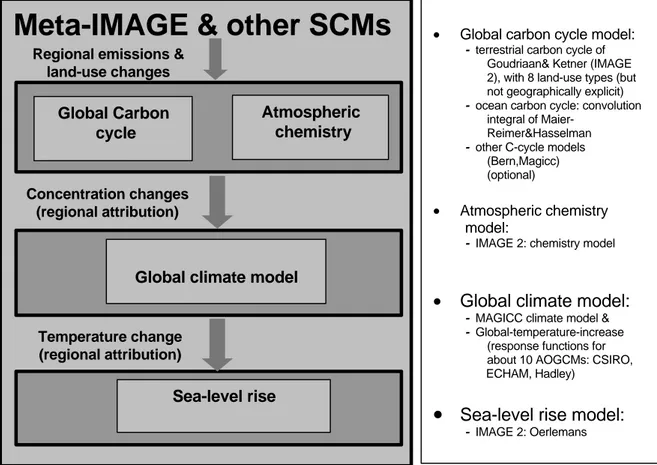
(12) Report 728001012. Page 12 of 41. In our view, the central question in this issue is: Does the present state of knowledge permit evaluating individual parties’ contribution to the climate change problem within an acceptable uncertainty range? Of course, we will leave it to the reader to decide what uncertainty is “acceptable”. Our present analysis concentrates on several important sources of uncertainty that can be quantified with the present modeling tools. More specifically, we will evaluate uncertainties in carbon-cycle and climate modeling, as well as specific methodological aspects as discussed in the Expert Meeting. We will assess their impacts on calculations of regional contribution to temperature increase and other climate indicators, such as sea-level rise and rate of temperature increase. A simple climate assessment model was developed for this purpose; it calculates the concentrations of greenhouse gases, radiative forcing, temperature and sea-level rise. To complement this model, we have developed a climate “attribution” module to calculate the regional contributions to various categories of emissions, concentrations of greenhouse gases, and temperature and sea-level rise. The thirteen world regions considered are: Canada, USA, Latin America, Africa, OECD-Europe, Eastern Europe, CIS, Middle East, India and South Asia, China and centrally planned Asia, West Asia, Oceania and Japan. The methodology can be extended to country level, as already done for a selected group of eleven countries (i.e. Australia, England, Germany, Japan, The Netherlands, USA, Brazil, China, India, Mexico and South Africa in Den Elzen et al. (1999). The model projections in the analysis presented here will only focus on the global, Annex I/non-Annex I and regional levels. This study follows the Brazilian Proposal in focusing on the regional anthropogenic emissions of the major greenhouse gases regulated in the Kyoto Protocol (i.e. carbon dioxide (CO2), methane (CH4) and nitrous dioxide (N2O)). Here and in the Brazilian Proposal, the term “anthropogenic emissions” is used for the net anthropogenic emissions of greenhouse gases or the difference between anthropogenic emissions by sources and direct anthropogenic removals by sinks of greenhouse gases. The other greenhouse gases included in the Kyoto Protocol i.e. hydrofluorocarbons (HFCs), perfluorocarbons (PFCs) and sulphur hexafluoride (SF6), are not taken into account since no regional emission data are available. The anthropogenic emissions of these gases, and the other halocarbons, i.e. CFCs, methyl chloroform, carbon tetrachloride, halons and HCFCs (Montreal Protocol), ozone precursors and SO2 (Clean Air protocols), as well as the natural emissions of all greenhouse gases, are considered at the global level only. Figure 1 depicts the climate assessment model, as used for the model analysis. At the core of the simple climate assessment model is the integrated simple climate model, meta-IMAGE 2.1 (henceforth to be referred to as meta-IMAGE) (Den Elzen, 1998; Den Elzen et al., 1997). MetaIMAGE is a simplified version of the more complex climate assessment model IMAGE 2. The latter aims at a more thorough description of the complex, long-term dynamics of the biosphereclimate system at a geographically explicit level (0.5o x 0.5o latitude-longitude grid) (Alcamo, 1994; Alcamo et al., 1996; 1998). Meta-IMAGE is a more flexible, transparent and interactive simulation tool that adequately reproduces the IMAGE-2.1 projections of global atmospheric concentrations of greenhouse gases, along with the temperature increase and sea-level rise for the various IMAGE 2.1 emissions scenarios. Meta-IMAGE consists of an integration of a global carbon cycle model (Den Elzen et al., 1997), an atmospheric chemistry model (Krol and Van der Woerd, 1994), and a climate model (upwelling-diffusion energy balance box model of Wigley and Schlesinger (1985) and Wigley and Raper (1992)). This core model has been supplemented with the following new elements: (i) the revised Brazilian model (Filho and Miquez, 1998), (ii) a climate “attribution” module and (iii) global temperature impulse response functions (IRFs, e.g. Hasselmann et al., 1993) based on simulation experiments with various Atmosphere-Ocean General Circulation Models (AOGCMs) for alternative temperature increase calculations. We have also implemented the global carbon cycle model of the MAGICC (Wigley, 1993) and Bern model (Joos et al., 1996) solely for the purpose of alternative CO2 concentration calculations in the model analysis presented here. This climate assessment model forms an integral part of our overall FAIR model (Framework to Assess.

(13) Report 728001012. Page 13 of 41. International Regimes for burden sharing), which was developed to explore options for international burden sharing, including the Brazilian approach (Den Elzen et al., 1999). This report is built up as follows. Chapter 2 briefly describes the background and modeling approaches used for calculating the concentrations, radiative forcing, temperature and sea-level rise projections. The model analysis on the uncertainties (Chapter 3) first assesses the impact of various carbon balancing mechanisms on regional contribution to global temperature increase. This involves balancing the past carbon budget within the range of IPPC estimates for the terrestrial and oceanic uptake, and for CO2 emissions from land-use changes. In addition, alternative carbon cycle model calculations are performed. Subsequently, we will assess the role of uncertainties in climate response to radiative forcing, i.e. different global temperature response functions. Results of both exercises will be combined to assess overall uncertainties. Chapter 4 assesses the impact of methodological choices, i.e. alternative climate indicators (rate of temperature increase and sealevel rise), Enting’s (1998) methodoloy of attributing non-linear radiative forcing, including other than fossil CO2 emissions, such as CO2 emissions from land-use changes and anthropogenic CH4 and N2O emissions, and the impact of the composition of the group of regions among which responsibility is shared (world vs. Annex-I). Chapter 5 concludes our evaluation.. Meta-IMAGE & other SCMs. •. Atmospheric chemistry. Global Carbon cycle. Concentration changes (regional attribution). Global carbon cycle model: - terrestrial carbon cycle of Goudriaan& Ketner (IMAGE 2), with 8 land-use types (but not geographically explicit) - ocean carbon cycle: convolution integral of MaierReimer&Hasselman - other C-cycle models (Bern,Magicc) (optional). Regional emissions & land-use changes. •. Atmospheric chemistry model: - IMAGE 2: chemistry model. Global climate model. • Temperature change (regional attribution). Sea-level rise. Global climate model: - MAGICC climate model & - Global-temperature-increase (response functions for about 10 AOGCMs: CSIRO, ECHAM, Hadley). • Sea-level rise model: - IMAGE 2: Oerlemans. Figure 1. The climate assessment model of FAIR as used for the model analysis..

(14) Report 728001012. Page 14 of 41.

(15) Report 728001012. 2 2.1. Page 15 of 41. Modeling approach for attributing anthropogenic climate change From emissions to concentration. Global concentrations of greenhouse gases The emissions of a greenhouse gas and its subsequent removal from the atmosphere determine the concentration. The lifetime of a greenhouse gas indicates the efficiency of the removal process and is a measure of the time that passes before an emission pulse is removed from the atmosphere. For nitrous dioxide (N2O) and the halocarbons, the rate of removal is linearly dependent on the concentration of the compound, and is derived by multiplying the concentration by a constant lifetime factor, as adopted in most current IPCC SCMs (Harvey et al., 1997). The rate of change for the concentration is then expressed as: dρ g dt. =. cv g E g. −. ρg /τ g. (1). where ρg is the atmospheric concentration of greenhouse gas g, Eg the anthropogenic emissions, τg the atmospheric exponential decay time or lifetime (yr) and cvg a mass-to-concentration conversion factor. For meta-IMAGE, the lifetime of the HCFCs, HFCs and CH3CCl3 is also a function of the tropospheric OH concentration. For the major greenhouse gases CO2 and CH4, the SCMs differ with respect to the modeling of the translation between the emissions and concentrations; this will be described in the overview below. Carbon dioxide - The carbon cycle is an integral part of the climate system, governing the changes of atmospheric CO2 concentration in response to the anthropogenic CO2 emission from fossil-fuel burning and land-use changes. This entanglement of climate system and carbon cycle gives rise to a range of uncertainties, which is reflected by the wide variety of existing modeling approaches. Global-mean carbon-cycle models consist of a well-mixed atmosphere linked to oceanic and terrestrial biospheric compartments. These models, driven by the anthropogenic CO2 emissions, calculate the terrestrial and oceanic sinks and the resulting atmospheric CO2 build-up. The oceanic component of simple carbon-cycle models can be formulated as an upwellingdiffusion model (Siegenthaler and Joos, 1992), or be represented by a mathematical function (known as a convolution integral), which can be attuned to closely replicate the behavior of more complex oceanic models (Harvey, 1989). The carbon-cycle models of MAGICC (Wigley, 1991), meta-IMAGE (Den Elzen, 1998) and the revised Brazilian model use the latter approach. The Bern carbon-cycle model (Joos et al., 1996) uses a more accurate representation of a convolution integral, i.e. an ocean mixed-layer pulse response function (surface deep-ocean mixing) in combination with a equation describing air−sea exchange. The terrestrial component in carbon cycle models is vertically differentiated into carbon reservoirs (Harvey, 1989), such as two living biomass boxes, a detritus and a soil box as in MAGICC (Wigley, 1993). In meta-IMAGE, the four terrestrial carbon boxes model (biomass, litter/detritus, humus, soil) is further differentiated horizontally into eight land-use types, i.e. forests, grasslands, agriculture and other land for the developing and industrialized world (Elzen, 1998). This allows us to analyze the effect of land-use changes such as deforestation on the global carbon cycle. The Bern model uses a decay-response function describing the carbon cycling in the terrestrial reservoirs in combination an equation describing the net primary production. The revised Brazilian model ignores the terrestrial carbon cycle, and only focuses on the slow oceanic carbon dynamics. To obtain a balanced past carbon budget of anthropogenic CO2 emission in these carboncycle models, and therefore a good fit between the historically observed and simulated atmospheric.

(16) Report 728001012. Page 16 of 41. CO2 concentration, it is essential to introduce terrestrial sinks (Schimel et al., 1995) in addtion to oceanic sinks. In the MAGICC model, the past carbon budget is solely balanced by the CO2 fertilization effect on the terrestrial biosphere, whereas in meta-IMAGE, temperature feedbacks on net primary production and soil respiration are also present. Although the N fertilization feedback was included in the earlier version of the meta-IMAGE model (Den Elzen et al., 1997), it is now excluded due to the need for it to be consistent with IMAGE 2.1 (Den Elzen, 1998), as well as with the new scientific insights of Nadelhoffer et al. (1999). Based on recent N-15 tracer studies, Nadelhoffer et al. concluded that it is unclear whether elevated nitrogen deposition is the primary cause of C sequestration in northern forests. To evaluate the climate-change related terrestrial feedbacks on a process base and with the necessary geographical explicitness, a more complex model like the IMAGE 2.1 model should be used (Alcamo et al., 1996; 1998). Here we use the insights gained from experiments with the IMAGE 2.1 model to find a parameterization of the CO2 fertilization and temperature feedbacks in meta-IMAGE. The modeling of these feedback mechanisms affects the future CO2 concentration projections. Various model parameterizations of these feedbacks, each leading to a balanced past carbon budget in carbon cycle models, can be shown to result in a wide range of future CO2 concentration projections (Schimel et al., 1995). This is caused by the carbon balancing procedure’s influence on the relative amount of carbon uptake by fast and slow overturning reservoirs. A disadvantage of a simple model framework is the inability to capture potentially important non-linear or “extreme” events. However, information can be drawn from more complex models, which can be used in a simpler model. An example is provided here by evaluating an additional large source of uncertainty. Preliminary results of experiments using global dynamic vegetation models suggest that the influence of climatic change on (land) vegetation in some Dynamic Global Vegetation Models might result in a shift of its functioning as a CO2 sink to a source in the second half of the next century (Cramer et al., in press). As an extreme example, we will apply an idealized representation of the results of one such model (White et al., 1999). The projected large decrease in sink size for this model might be explained by the large forest fraction in the simulation of present-day land cover, making the model relatively sensitive to drought. To reflect this model’s results in an idealized experiment, we will linearly decrease carbon uptake by the terrestrial vegetation in meta-IMAGE (as represented by Net Ecosystem Productivity [NEP]) from the value it has in 2050 to 0 in 2100 (see section 3.2). Methane - The chemical removal rate and atmospheric lifetime of CH4 depend on the concentration of CH4 itself, and are also affected by the concentrations and emissions of the gases NOx, CO and VOCs, and the tropospheric concentration of OH. The current lifetime is about nine years (Harvey et al., 1997). In addition to removal by chemical reactions in the atmosphere, CH4 is also absorbed by soils, with a specific time constant of 150 years. In meta-IMAGE the CH4 lifetime is a function of the transport losses to both stratosphere and biosphere, and the average atmospheric residence time. This function depends on the OH concentration (Krol and Van der Woerd, 1994). In MAGICC this residence time depends only on the emissions of CH4 itself (Osborn and Wigley, 1994). In the revised Brazilian model, a constant CH4 lifetime is used. Concentrations attributed Caculations of regional contributions to concentration increases can be done in a straightforward manner using the mass balance equation (1) with regional anthropogenic emissions and a regional sink term. This is calculated as: ρg,r(t)/τg(t), in which ρg,r(t) is the regional atmospheric concentration of greenhouse gas g at time t. As mentioned above, only the major greenhouse gases, i.e. CO2, CH4 and N2O, are accounted for in calculating contributions of regions, whereas the influence of emissions of the other greenhouse gases and aerosols are considered at global level..

(17) Report 728001012. 2.2. Page 17 of 41. From concentration to radiative forcing. Global radiative forcing Increased concentrations of greenhouse gases in the atmosphere lead to a change in radiative forcing, a measure of the extra energy input to the surface-troposphere system. As the concentration of a greenhouse gas increases, this dependence of forcing on concentration will gradually ”saturate” in certain absorption bands. An additional unit increase of concentration will gradually have a relatively smaller impact on radiative forcing. At present-day concentrations, the saturation effect is greatest for CO2 and somewhat less for CH4 and N2O. Additionally, some greenhouse gases absorb radiation in each other’s frequency domains. This “overlap effect” is especially relevant for CH4 and N2O. Increases in CH4 concentration decrease the efficiency of N2O absorption and vice versa. The present SCMs such as MAGICC and meta-IMAGE use the global radiative forcing dependencies of the IPCC (Harvey et al., 1997), including the major saturation and overlap effects. In our present study, we will not include uncertainties in radiative forcing, as these are considered relatively low for the major greenhouse gases included here (IPCC, 1995). Radiative forcing attributed Calculating regional contributions to global radiative forcing by a greenhouse gas is more complicated than contributions to concentration increases. Due to the saturation effect, the radiative forcing of each additional unit of concentration from the ”early emitters” (no saturation of CO2 absorption) is larger than the radiative forcing of an additional unit from the ”later emitters” (partial saturation of CO2 absorption). When more regions start to contribute, a decision will have to be made on how to divide the “benefit” of the overlap or saturation, otherwise the sum of the partial effects would exceed the whole radiative effect (Enting, 1998). The resulting regional radiative forcing depends on the methodology followed. There are two possibilities: the radiative forcing (Qg in W⋅m-2) may be calculated in proportion to (i) attributed concentrations of a greenhouse gas, or (ii) the changes in attributed concentrations. The methodology of (ii), the non-linear approach to calculate contributions to radiative forcing, is described in Enting (1998): t. Q g (r ) =. ∫. dq g dρg. d ρ g (r ) dt ' dt '. (2). where qg(ρg) is the radiative forcing function of greenhouse gas, g, depending on its concentration, ρg. Each component accounts for the importance of each year’s radiative effect, depending on the total contributions from all regions over previous years (through the use of the time-dependent factor dqg/dρg). Similar to calculating contributions to concentration increases, only CO2, CH4 and N2O are accounted for here. This implies that the total radiative forcing consists of the sum of radiative forcings caused by the CO2, CH4 and N2O emissions for individual regions, and the overall radiative forcing caused by the global emissions of the other greenhouse gases and aerosols (a separate category). The first methodology ignores the partial saturation effect and considers equal radiative effects of the ”early emitters” and the ”late emitters”, whereas the second includes this partial saturation effect, implying a larger radiative effect of the “early emitters” (Annex I regions). In this report the first methodology has been adopted for the further base calculations. In a later sensitivity analysis we will assess the impact of the second methodology on a region’s contribution to anthropogenic climate change..

(18) Report 728001012. 2.3. Page 18 of 41. From radiative forcing to temperature increase. Global mean surface-air temperature increase The large heat capacity of the oceans plays an important role in the time-dependent response of the climate system to external forcing. Transport of heat to the deep ocean layers effectively slows down the surface-air temperature response over ocean and land surfaces, as well as in the atmosphere. If the time horizon of a climate change analysis only extends over a few years or decades, the response is, however, dominated by the upper ocean surface layer, reaching relatively rapid adjustment within a few decades. Still, a significant part, roughly 50 percent, of the final global warming will manifest itself decades to centuries later. The delay caused by penetration of heat to the deeper ocean layers is also what causes sea-level rise to continue long after stabilization of greenhouse gas concentrations (Wigley and Raper, 1993). The balance between the rapid and slow adjustment terms is a source of uncertainty, as it depends on non-linear processes like stratification of the upper ocean layers. The climate sensitivity is another important source of uncertainty in climate response to external forcing. We will use the IPCC (1995) definition, the long-term (equilibrium) annual and global-mean surface-air temperature increase for a doubling CO2 concentration, denoted by ∆T2×. The climate sensitivity is an outcome of all geophysical feedback mechanisms and their associated uncertainties. The most important source of uncertainty is the hydrological cycle, in particular, clouds and their interaction with radiative processes. IPCC (1995) has estimated the climate sensitivity to lie within the range of 1.5 to 4.5 °C, with a “best-guess” value of 2.5 °C. Physically, the most rigorous way to analyze climate system response to anthropogenic forcing is provided by ”state-of-the-art” AOGCMs. Because they are computationally expensive, these 3-dimensional climate models are difficult to apply in multiple-scenario studies, uncertainty assessments and analysis of feedbacks. In such studies, generally simpler models are applied (e.g. Harvey et al., 1997). As a reference case in our calculations, we will use the upwelling-diffusion box climate model originally described in Wigley and Schlesinger (1985) and updated in Wigley and Raper (1992), as implemented in meta-IMAGE. Our model version uses a default climate sensitivity of ∆T2×=2.35 °C to match IMAGE 2.1 results. For alternative calculations of temperature response, we will derive parameters from a range of AOGCMs to be used in Impulse Response Functions (IRFs). As explained in Hasselmann et al. (1993), IRFs form a simple tool for mathematically describing (“mimic”) transient climate model response to external forcing. A two-term IRF model used here (as in Hasselmann et al., 1993) is based on the following convolution integral, relating temperature response ∆T to time-dependent external forcing Q(t):. ∆ T (t ) =. ∆ T 2× Q 2×.  2 − ( t − t ') / τ s  Q ( t ' )  ∑ l s (1 / τ s ) e  dt ' ∫t0  s =1  t. (3). where Q2× is the radiative forcing for a doubling of CO2 and ls the amplitude of the 1st or 2nd component with exponential adjustment time constant τs, while l1 + l 2 = 1 . ∆T2×/Q2× equals the climate sensitivity parameter λ (Cess et al., 1989). In an alternative formulation, we can define C=1/λ, and characterize C as the effective heat capacity of the climate system, including climate response feedbacks. The IRF model is mathematically equivalent to a (multi-)box energy balance climate model. Note that in the IRF description these boxes respond independently to the forcing. This makes it impossible to readily link the different IRF terms to specific elements in the physical climate system, like mixed layer and deeper ocean (Hooss et al., 1999). Because we have not found elaborate comparisons of IRF “performance” for a range of AOGCMs in the literature, we will discuss this approach and the problems we encountered below. Results from a long HadCM2 AOGCM stabilization run (Senior and Mitchell, submitted to J. Clim.) suggest that climate sensitivity crucially depends on the state of the climate system. The climate sensitivity in this AOGCM experiment changes from about 2.6 °C over the first 200 years to.

(19) Report 728001012. Page 19 of 41. 3.8 °C after 900 years. Using IRFs with a constant climate sensitivity, as was done here, does not reflect such a model’s behavior. Note that a higher sensitivity to radiative forcing later on in the experiment suggests a potentially important “reversed saturation” effect (as opposed to the saturation of radiative forcing, resulting in steadily decreasing sensitivity). In contrast, another study (Watterson, 2000) suggests a steadily increasing effective heat capacity of the climate system. Because of the inverse proportionality of ∆T2× and C as defined here, the sign of the effect found is opposite, resulting in a weaker response to forcing later on in the experiment. Both studies suggest that a simple model, mimicking AOGCM response, performs better when either climate sensitivity or heat capacity is made time-dependent. In this paper, we have used a constant ∆T2× and simply calculated the best fit over a multi-century period of each model’s results. For HadCM2, we calculated over this period an average value of 3 °C of the diagnosed climate sensitivity from Senior and Mitchell (submitted). For the other models, we will use the climate sensitivity from the literature. We applied least-square fitting to determine values for the constants ls and τs, as presented in Table 1; this allows the IRF model to closely mimic the temperature response in a specific AOGCM climate change experiment. We also included experiments with the simpler climate model of IMAGE 2.1 (Haan et al., 1994). In these experiments, we used two different values for the vertical diffusion coefficient in the ocean, which about span the values for simple climate models found in the literature (e.g. Schlesinger and Jiang, 1990). This parameter might be used to calibrate such upwelling-diffusion energy-balance climate models to emulate AOGCM response. In Table 1 we include references and the aliases under which the various models are mentioned throughout this report. The range of IRF parameters will provide us with an estimate of the possible range of uncertainty in the dynamics of climate system response to the applied transient forcing. Note that using a model intercomparison in uncertainty assessment has two major shortcomings. First, we are unable to supply information on the probability distribution of the results. Second, there is no guarantee that the choice of model experiments will be complete in covering the full range of plausible outcomes. As an example of IRF performance, Figure 2 shows results from the CSIRO GCM experiment (Watterson, 2000) and the IRF model using the appropriate parameter values. Both models were forced with the same scenario (see Table 1). For all IRF fits, we compared the RootMean-Square (RMS) error value of the fit to the standard deviation, if available, of global mean surface-air temperature in the control run of the AOGCMs (using constant present-day or preindustrial greenhouse gas concentrations). The latter is a measure or natural variability, which is not captured by the IRFs, as can also be seen in Figure 2. Therefore, a fit using IRFs will make a RMS error at least as large as the standard deviation of the control run. In general, the RMS error of the IRF fit did not differ significantly from the standard variation of surface-air temperature in the AOGCM control run. However, this check on RMS of the very same scenario to which the IRF model was tuned is very limited as a performance test. Because of non-linearities in the system, which are not captured by the IRF model, the values found for the IRF constants will vary when the same AOGCM is driven by a different greenhouse gas concentration scenario (see also Hasselmann et al., 1993). The IRF modeltuned to one AOGCM scenario run will therefore have a larger error when both models are forced with a different scenario. As a test, we used two different stabilization runs of the GFDL AOGCM (Manabe and Stouffer, 1994; denoted by GFDL ’93 in this report). Where the 2xCO2 GFDL ’93 run shows a weakening of the thermohaline circulation (as indeed does the majority of coupled GCMs), the 4xCO2 run includes a collapse, identified as a potential “extreme event” (Stocker and Schmittner, 1997). However, the parameters found for the two GFDL ’93 runs do not differ significantly (Table 1). The last problem we encountered was that when IRF parameters are diagnosed from a longer GCM run, the balance of fast and slow response terms tends to shift to longer time scales. As our analysis spans a few centuries, we decided to take the first 500 years of the climate model experiments, or less than that if 500 years were not available (Table 1). We intend in future to apply.

(20) Report 728001012. Page 20 of 41. a simplified, computationally very efficient AOGCM (ECBilt; Opsteegh et al., 1998) to better assess the size of the errors made with this IRF approach. To highlight the importance of the balance between fast and slow response terms, in Figure 3 we show the response of the IRFs to a sudden doubling of CO2 concentration. Note that due to the scenario dependence of IRF fits mentioned above, the IRF responses to this sudden doubling of CO2 resemble only the ”original” climate model response to such forcing when the same, extreme, scenario was used when determining IRF parameters. The spread of IMAGE 2.1 results show that adjusting parameters in simple climate models may offer another way to mimic AOGCM response, as extensively shown in Senior and Mitchell (submitted) for example. Also indicated in Figure 3 is Table 1 Summary of climate model experiments used to derive Impulse Response Functions and values of IRF parameters Climate model Reference Short description of model Climate l1 τ2 τ1 (aliases in this experiment sensitivity (yr) (yr) report) (°C)(3) ECHAM1/LSG(1) Hasselmann et al. Instantaneous CO2 doubling(2) 1.58 2.86 0.685 41.6 (1993) 7 ECHAM3/LSG Voss et al. (1998) 500 years used ; 1% per year CO2 2.5 14.4 0.761 393 increase till 4×CO2 is reached, then constant; total is 850 years GFDL ‘90(1) Hasselmann et al. Instantaneous CO2 doubling(2) 1.85 1.2 0.473 23.5 (1993) 3.5 6.5 0.671 388 Manabe and 1% per year CO2 increase till 2×CO2, GFDL ’93 2× Stouffer (1994) then constant; total 500 years Manabe and 1% per year CO2 increase till 3.5 8.5 0.665 233 GFDL ’93 4× Stouffer (1994) 4×CO2, then constant; total 500 years GFDL ‘97 Haywood et al. Two-member ensemble mean GHG3.7 12.6 0.613 145 (1997) only historical concentrations from 1760 till 1990, then IS92a; total 300 years HadCM2 Senior and 500 years used; 1% per year CO2 3.0 7.4 0.527 199 Mitchell increase till 2×CO2, then constant; (submitted to J. total 900 years Clim.) CSIRO Watterson (2000) 500 years used from historical GHG 3.6 12.7 0.605 432 forcing till 1990, then 1%/year CO2 increase till 3×CO2, then constant; total 565 years IMAGE 2.1 This report Instantaneous CO2 doubling(2) 2.37 2.19 0.654 76 2 (k=0.56 cm /s) IMAGE 2.1 This report Instantaneous CO2 doubling(2) 2.37 1.92 0.471 105 2 (k=2.3 cm /s) Brazilian Filho and Miguez 3.06 20 0.634 990 revised(1) (1998) (1). IRF parameters were not calculated here, but adopted from reference. In an “instantaneous CO2 doubling” experiment, the atmospheric CO2 concentration is doubled abruptly (2×CO2), with the climate model starting from a present-day equilibrium state. The concentration is then held fixed at 2×CO2, while the model is allowed to reach a new equilibrium. (3) Climate sensitivity was adopted from respective reference, except for HadCM2, where climate sensitivity is averaged over 500 years (Senior and Mitchell, submitted). (2).

(21) Report 728001012. Page 21 of 41. the response of the IRFs used in the revised Brazilian Proposal (Filho and Miquez, 1998). The parameters used there result in an “outlier” response, especially in the longer term (see also numeric values of IRF constants in Table 1), although not as extreme as reported in an earlier assessment of ours, based on a very limited set of AOGCM results (Den Elzen et al., 1999). Temperature increase attributed As mentioned in Section 2.2, global radiative forcing from a greenhouse gas (i.e. CO2, CH4 and N2O) is the sum of radiative forcings caused by emissions of individual regions. Therefore, Q(t’) in R. Equation (3) can be replaced by the sum over these regions,. ∑ Q (t ' ) . Placing this summation r =1. r. over regions outside of the convolution integral, we can apply Equation (3) to regional forcings to obtain “regional” temperature increase. All regional representations of Equation (3) thus obtained contain the same factor of ∆T2×. This factor cancels out when relative contributions are calculated by dividing individual regional terms by global temperature increase, which contains the same factor. This means that when determining relative contributions using our linearised approximation of the climate system response, uncertainty in climate sensitivity does not matter any longer. As we will further illustrate in section 3.3, the relative contribution as in the Brazilian Proposal depends only on the above-mentioned balance of processes on short and long time scales, determined by the IRF time-scale parameters ls and τs.. 5. 4. ∆T (K). 3. 2. 1. 0 1880. 1980. 2080. 2180. 2280. 2380. -1 year. Figure 2. The IRF model (heavy line) tuned to the CSIRO GCM data (light line) (Watterson, 2000) where the radiative forcing follows the IS92a scenario, starting with the historical pathway from 1881, and stabilises at 3× the present CO2 concentration..

(22) Report 728001012. Page 22 of 41. ∆T/∆T2xCO2 1. IMAGE 2.1 2xCO2 step 100 yr (K=0.56 cm2/s) IMAGE 2.1 2xCO2 step 100 yr (K=2.3 cm2/s) ECHAM1/LSG 2xCO2 step 100 yr ECHAM3/LSG +1%/yr Stab. 4xCO2 850 yr GFDL '90 2xCO2 step 100 yr GFDL '93 +1%/yr Stab. 2xCO2 500 yr GFDL '93 +1%/yr Stab. 4xCO2 500 yr GFDL IS92a-ensemble mean. 0.75. 0.5. HadCM2 IS92a-ensemble mean. 0.25. CSIRO IS92a Stab. 3xCO2 500 yr Brazilian revised. 0 0. 50. 100. 150. 200. year. Figure 3. The temperature response (normalized by climate sensitivity) to a sudden doubling of the atmospheric CO2 concentration at time t=0 for the various IRFs in Table 1..

(23) Report 728001012. 3. 3.1. Page 23 of 41. Model analysis of a region’s contribution to global warming: model uncertainties Introduction. In the analysis we will assess the impact of the following model uncertainties on a region’s contribution to global warming: (1) various balancing procedures of the past carbon budget and other carbon cycle models; (2) various climate response functions and (3) the overall impact of these uncertainties in the global carbon and climate models. For this analysis we use the climate assessment model as described in Chapter 2. The reference case of the calculations presented below always refers to the results of the meta-IMAGE model - the core of the climate assessment model - with its default parameter settings (Den Elzen, 1998). For this model, which starts in 1750, we assume an initial steady state before anthropogenic disturbances are imposed upon the system. The main input data of the model framework are composed of the following human-induced perturbations of the climate system: (1) anthropogenic (energy-, industrial and agriculture-related) emissions of greenhouse gases, (2) land-use changes and the associated CO2 emissions. These input data will be first briefly described.. 3.2. Input data. Anthropogenic emissions of greenhouse gases The regional fossil fuel CO2 emissions for the period 1751-1995 are based on the CO2 emissions database of the Oak Ridge National Laboratory (ORNL), which is also referred to as ORNLCDIAC (CO2 Data and Information Assessment Center) (Marland and Rotty, 1984; Marland et al., 1999a; Andres et al., 1999). The global bunker and feedstock emissions, and the difference between the global and total sum of regional CDIAC emissions are allocated to the regional CO2 emissions using the country contribution data of the EDGAR (Emission Database for Global Atmospheric Research) data set (Olivier et al., 1996; 1999); and the HYDE database (Klein-Goldewijk and Battjes, 1997) for the period 1890-1970. The ORNL-CDIAC emission data are limited to CO2 emissions from fossil fuels and cement production. The historical regional anthropogenic CH4 and N2O emissions (including the emissions due to land-use changes) are therefore taken from the EDGAR data set. The historical global anthropogenic emissions of the halocarbons, other greenhouse gases and ozone precursors are based on EDGAR (Olivier et al., 1999) and SO2 is based on Smith et al. (2000). The regional anthropogenic CO2, CH4 and N2O emissions, as well as the global emissions of the other greenhouse gases and SO2 for the 1995 to 2100 period are based on the IMAGE 2.1 Baseline-A scenario (Alcamo et al., 1998). This scenario is comparable with the IPCC IS92a emissions scenario. Land-use changes and associated CO2 emission The historical regional CO2 emissions from land-use changes are based on Houghton and Hackler (1995) and Houghton et al. (1983; 1987), with a further aggregation to the 13 regions according to regional past population trends. The global CO2 emissions estimate for the period 1850 to 1980 (115 GtC) and the 1980-1990 average flux (1.4 GtC⋅yr-1) are almost identical to the IPCC 1995 estimates (Schimel et al., 1995). A recent revised analysis of Houghton (1999) shows a somewhat higher estimate for the 1980s (2.0 GtC⋅yr-1), but an almost similar estimate for the 1850-1980 total flux. These revised regional emissions have not been adopted here, since we wanted to use the global carbon balance estimates of the IPCC 1995 scientific assessment (Schimel et al., 1995). The land-.

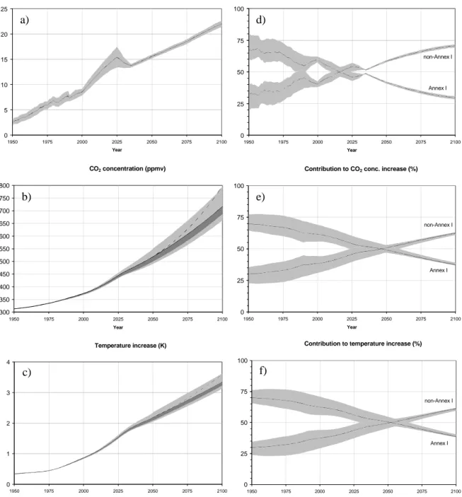
(24) Report 728001012. Page 24 of 41. use changes - important for the terrestrial carbon-cycling processes - are also based on Houghton and Hackler (1995), but further disaggregated in the four major land cover types: forests, grasslands, agriculture and other land, for the developing and industrialized world, as used in metaIMAGE. The area changes for the four land-use categories (forests, grasslands, agricultural and other land) in the developing and industrialized world for the period 1990-2100 are also based on aggregated land-use data of the Baseline-A scenario. The 1995-2100 regional CO2 emissions from land-use changes are also based on the Baseline-A scenario.. 3.3. Various balancing approaches for the past carbon budget. To investigate the sensitivity of the global CO2 concentration and temperature increase, and the contribution of specific regions (i.e. the Annex I and non-Annex I regions) for balancing the past carbon budget, we performed a sensitivity analysis using the global carbon cycle model of metaIMAGE. In the reference case, model parameters representing the key terrestrial feedbacks (i.e. the CO2 fertilization effect and temperature feedback on net primary production and soil respiration) and oceanic uptakes are set on the default values used within meta-IMAGE. This leads to a balanced past carbon budget and a good fit between the historically observed and simulated CO2 concentrations. The simulated carbon fluxes of the components of the carbon budget for the 1980s (1980-1989) are similar to the IPCC estimates (Table 2). The atmospheric CO2 concentration projection for the IS92a emissions scenario is about 690 ppmv in 2100, which is somewhat lower than the central IPCC and MAGICC projection of approximately 705-710 ppmv (revised 1994 carbon budget) (Schimel et al., 1995). The latter is a direct result of the assumed high CO2 fertilization effects and high agricultural carbon uptake within meta-IMAGE (both resulting from the consistency with IMAGE 2.1) (Den Elzen, 1998). Figures 4b&c give the projections of the CO2 concentration and temperature increase for the Baseline-A scenario. The temperature increase projection uses the total radiative forcing from changes in the concentrations of all greenhouse gases and aerosols as input. The resulting temperature increase for the reference case is about 3.1 oC for the period 1750 (pre-industrial) to 2100. In the following sensitivity experiments the scaling factors for the ocean flux, emissions from land-use changes, northern hemispheric terrestrial uptake, and CO2 fertilization feedback parameters, are varied so that the set of parameter combinations will lead to a well-balanced past carbon budget. The temperature feedback parameters are kept at their default values. The simulated carbon fluxes of the carbon budget, i.e. the oceanic and terrestrial carbon uptake, and the CO2 emissions from land-use changes during the 1980s, should be between the upper and lower boundaries of the IPCC estimates (Table 2). In the first two extreme "oceanic uptake" cases, a high and a low oceanic uptake, the scaling factors for the ocean flux are set at the maximum and minimum values. This results in the 1980s oceanic uptake of 3.0 and 1.0 GtC yr-1, respectively. The balanced past carbon budget is now achieved by scaling the CO2 fertilization feedback parameters and the northern hemispheric terrestrial uptake. The terrestrial sink for the 1980s then varies between 0.8 and 2.3 GtC yr-1 (Table 2). These two cases have been selected from other similar conditioned simulation experiments as two extreme examples of the balancing variations in the terrestrial and oceanic uptake fluxes (representing the terrestrial and oceanic uncertainties, in which the impact of variations in the temperature feedback parameters is ignored). The resulting projected CO2 concentration range in 2100 varies between 687 and 719 ppmv (717 ppmv for the reference case). The following experiments consider the uncertainties in the CO2 emissions from land-use changes (land-use sources and carbon sink uncertainties) by setting its scaling factor at maximum and minimum values (emissions during the 1980s between 0.6-2.6 GtC yr-1) (Table 2). The extreme upper and lower CO2 concentration projections are now achieved (662 and 794 ppmv, respectively,.

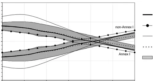
(25) Report 728001012. Page 25 of 41. by 2100), by balancing the past carbon budget with only the CO2 fertilization effect, while the oceanic parameters are kept constant. Figures 4d-f depict the Annex I and non-Annex I contributions to global anthropogenic CO2 emissions, CO2 concentration, and temperature increase and uncertainty ranges based on these sensitivity experiments. Taking the central reference case, the moment of convergence of Annex I and non-Annex I contributions is shown to be delayed from 2015 (anthropogenic CO2 emissions) to 2045 (CO2 concentration) to 2050 (temperature increase). Uncertainties in the terrestrial and oceanic uptake do not affect the contribution outcomes. However, when also the uncertainties in the CO2 emissions from land-use changes are included, the convergence year of equal Annex I and nonAnnex I contribution to temperature increase varies between 2030 and 2065. The uncertainty range of Annex I contribution to the 1990 temperature increase becomes 57% to 75% (65% for the reference case). Over time, the influence of the uncertainties in the land-use CO2 emissions on the contribution projections decreases rather quickly, mainly due to the dominating role of fossil fuel CO2 emissions in the total anthropogenic CO2 emissions, but also to the decay of past (uncertain) emissions. After 2025 the uncertainties in the contribution projections become even almost negligible. The anthropogenic CO2 emissions are then almost entirely (about 95%) determined by the fossil CO2 emissions, which are more than double the 1995 value, whereas the land-use emissions somewhat stabilizes at about 50% of its present value (See also Figure 4a). As mentioned in section 2.1, we have implemented an idealized form of a carbon “sink-tosource shift” of the terrestrial biosphere after 2050. The dashed line in Figure 4 clearly indicates the consequences of such a shift. However, this does not show up at all in the representation of the contributions. The increase in atmospheric CO2, as compared to a case without a “sink-to-source shift”, is not attributed to any specific region and only exerts an influence through a lengthening of atmospheric CO2 lifetime. This is combined with the contribution of a region being determined by emissions in a period of more than a hundred years before an evaluation point. Therefore changes in CO2 lifetime at the very end of this assessment might not have a significant effect. We also did the experiments for the reference case implementing the IPCC Bern carbon cycle model, as described in Joos et al. (1996), and the MAGICC carbon cycle model, as described in Wigley and Raper (1992) and Wigley (1991). The first results for the Annex I and non-Annex I contributions to the temperature increase for these two cycle models show almost the same results as the meta-IMAGE model. Table 2 Components of the carbon budget (in GtC⋅yr-1) based on model simulations for the carbon balancing experiments for the period 1980-1989 according to the IPCC (Schimel et al., 1995). Component. CO2 emissions from fossil fuel burning and cement production (Efos) CO2 emissions from land-use changes (Eland) Change in atmospheric CO2 (dCCO2/dt) Uptake by the oceans (Soc) Uptake by Northern Hemisphere forest regrowth (Efor) Additional terrestrial sinks (IPCC: [Efos+Eland ] - [dC/dt*+ Efor +Soc]). IPCC estimate. Reference case. High oceanic uptake. Low oceanic uptake. High deforestation. Low deforestation. 5.5 + 0.5 1.6 + 1.0 3.3 + 0.2 2.0 + 0.8 0.5 + 0.5. 5.5 1.6 3.3 2.0 0.5. 5.5 1.6 3.3 3.0 0.0. 5.5 1.6 3.3 1.0 0.5. 5.5 2.6 3.3 2.0 0.5. 5.5 0.6 3.3 2.0 0.5. 1.3 + 1.6. 1.3. 0.8. 2.3. 2.3. 0.3.

(26) Report 728001012. Page 26 of 41 Contribution to CO2 emissions (%). CO2 emissions (Gt/yr). 100. 25. a). d). 20. 75 non-Annex I. 15. 50 10. Annex I. 25 5. 0. 0. 1950. 1975. 2000. 2025. 2050. 2075. 2100. 1950. 1975. 2000. Year. 2050. 2075. 2100. Year. CO2 concentration (ppmv). Contribution to CO2 conc. increase (%). 800 750. 2025. 100. b). e). 700 75. 650. non-Annex I. 600 550. 50. 500 Annex I. 450 25. 400 350 0. 300 1950. 1975. 2000. 2025. 2050. 2075. 2100. 1950. 1975. 2000. 2025. 2050. 2075. 2100. Year. Year. Contribution to temperature increase (%). Temperature increase (K). 100. 4. f). c) 75. 3. non-Annex I. 2. 50. 1. 25. Annex I. 0 1950. 0 1975. 2000. 2025 Year. 2050. 2075. 2100. 1950. 1975. 2000. 2025. 2050. 2075. 2100. Year. Figure 4. The global anthropogenic CO2 emissions, CO2 concentration and temperature increase (left column) and the contribution of Annex I and non-Annex I (right column) for the Baseline-A scenario according to the meta-IMAGE model for the carbon balancing experiments (solid line). The two uncertainty ranges represent the uncertainties in the terrestrial and oceanic carbon sink fluxes (dark-grey), and in the sink and land-use sources (light-grey). The temperature increase is calculated using as input the total radiative forcing from changes in the concentrations of all greenhouse gases and aerosols. Also indicated is the terrestrial “sink-to-source shift” case (dashed line)..

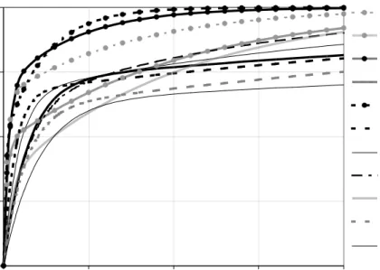
(27) Report 728001012. 3.4. Page 27 of 41. Using temperature response functions of various AOGCMS. As explained in section 2.3, we will apply the results of a number of climate models to reflect uncertainty in climate modelling. Figure 3 has already illustrated the spectrum of response time scales diagnosed from the AOGCM experiments. Using this range of different response time scales and the differing climate sensitivities of the AOGCMs, we will show the resulting spread in projected temperature response in Figure 5a. The results of the IRF models, forced by our BaselineA scenario, are not equal to the responses in the “original” climate model experiments, as other scenarios were used there (see Table 1). For example, our reference scenario results in 7.4 Wm-2 radiative forcing in 2100, compared to, for example, about 6.3 W⋅m-2 as given by IPCC (1995) for IS92a, or 8.8 W⋅m-2 in the HadCM2 experiment (Viner, pers. comm.). Differing climate sensitivity of the models is the main factor behind the range of results in Figure 5a, as we will show later on. This also applies to rate of temperature increase as shown in Figure 5b. Models with a fast response do not necessarily show a greater rate of temperature increase, because of their relatively low climate sensitivity (compare, for example, ECHAM1/LSG or GFDL ’90 in Figure 5b with Figure 3). In Figure 6a, the solid line represents the temperature response of our meta-IMAGE reference case, which is not necessarily the most likely. In this figure, the innermost, dark-grey area depicts the range of results if all the different IRF time-scale parameters (τs and ls in Equation (3) and Table 1) are applied using the same IPCC “best-guess” climate sensitivity of 2.5 °C. The uncertainty range broadens significantly if the IRF time-scale parameters are combined with their respective climate sensitivities in Table 1, ranging from 1.58 to 3.7 °C (grey, compare with Figure 5a). Finally, the range broadens even further if the IRF time-scale parameters are arbitrarily combined with climate sensitivities from the full IPCC range of 1.5 – 4.5 °C (light grey). Note that this exercise of combining time-scale parameters with arbitrary climate sensitivities does not necessarily result in the IRF model being able to reproduce the observed temperature increase of about 0.6 °C (IPCC, 1995) up to 1990. This is directly connected to the issue of uncertainty in sulphate aerosol forcing, for which we assume central values for direct forcing only (IPCC, 1995), and natural forcings, which are not included here. Combining high climate sensitivity, resulting in a strong response to greenhouse gas concentration increases, with strong sulfate aerosol forcing might very well result in a close reproduction of the historical pathway (see, for example, Tett et al., 1999). Figure 6a clearly shows the climate sensitivity as playing a dominant role in determining the range of absolute temperature increase. However, in Figure 6b, we follow the same procedure of including more and more sources of uncertainty for relative contributions of Annex I and nonAnnex I parties to temperature increase. This time, the uncertainty range expands no further than the dark-grey area, resulting from the spread in response time-scales alone. As a result, the range of Annex I contributions in 2100 is determined as comprising 39.5–42.1 percent, determined solely by the range of dynamic responses of the AOGCMs reviewed here. In our scenario, convergence of contributions of Annex I and non-Annex I is realised between 2053 and 2062. We now clearly see, as previously explained, that uncertainty in climate sensitivity plays no role when assessing relative contributions. However, we would like to stress again that the climate sensitivity remains a crucial link between emission control, and climate and other impacts. We can also see that over time, the influence of various global temperature response functions on the contribution projections increases. Studying the contribution projections for individual regions teaches us that the influence is particularly large for countries exhibiting fastgrowing emissions, i.e. China and India (non-Annex I regions). With the time delay characteristic of the climate system, the range of temperature projections is in the first order proportional to the growth rate of emissions. This will be further explained in the next section..

(28) Report 728001012. Page 28 of 41 Rate of Temperture change (K/decade). Temperature change (K) 6. 0.5. b). a) 5. 0.4. 4. 0.3 3. 0.2 2. 0.1. 1 0. 0. 1950. 1975. 2000. 2025. 2050. 2075. 2100. 1950. 1975. 2000. Year. 2025. 2050. 2075. 2100. Year. Figure 5. The temperature increase (a) and the rate of temperature increase (b) for the Baseline-A scenario using the CO2 concentration pathway from the reference case according to the metaIMAGE climate model and various IRFs of AOGCMs. The outcome of IMAGE 2.1 (K=2.3 cm2⋅s-1), similar to ECHAM3/LSG is not shown here so as to avoid confusion. See Figure 3 for the legend.. Contribution to temperature increase (%). Temperature increase (K) 6. 100. a). b). 5. 75 4. non-Annex I. 3. 50 Annex I. 2. 25 1 0 1950. 0 1975. 2000. 2025 Year. 2050. 2075. 2100. 1950. 1975. 2000. 2025. 2050. 2075. 2100. Year. Figure 6. The temperature increase (a) and the contribution to global temperature increase of Annex I and non-Annex I (b) for the Baseline-A scenario using the CO2 concentration pathway from the reference case according to the meta-IMAGE climate model (heavy line) and IRFs of AOGCMs. Dark-grey: range of outcomes for IPCC’s (1995) “best-guess” climate sensitivity of 2.5 °C combined with the IRF time-scale parameters of the AOGCMs. Grey: IRF time-scale parameters combined with their respective climate sensitivities from Table 1. Light-grey: IRF time-scale parameters arbitrarily combined with climate sensitivities in the full IPCC (1995) range of 1.5 – 4.5 °C..

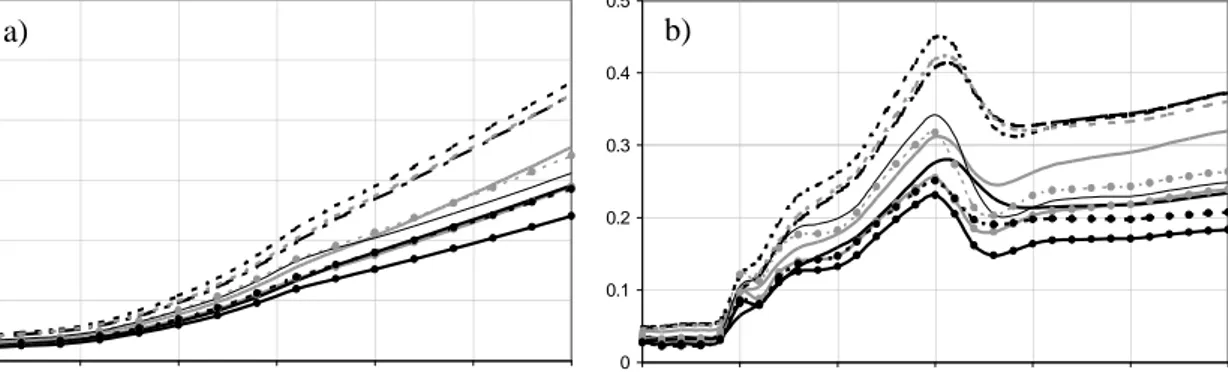
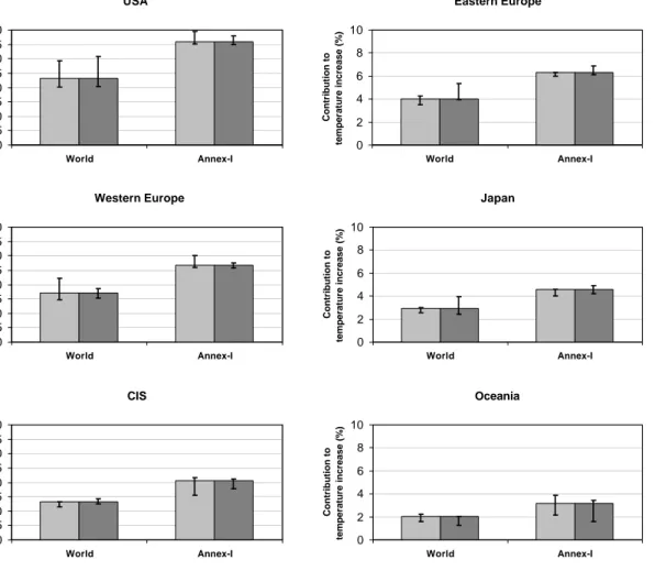
(29) Report 728001012. 3.5. Page 29 of 41. Overall uncertainties of global carbon cycle and climate models. Having analyzed the effect of some major uncertainties in the carbon cycle and climate in the preceding sections, we will now compare their relative importance for projected temperature increase. In Figure 7a, the central dark-gray area depicts total uncertainty in the carbon cycle balancing exercise (compare with Figure 4), while the gray area reflects total uncertainty from climate modeling (compare with Figure 6). The light-gray area shows the resulting total range in outcomes using the overall uncertainties in the carbon cycle and climate. The extension of uncertainty on the upper side is worth noting; this is a result of the strong temperature feedback on soil respiration as it is triggered by a high temperature increase in meta-IMAGE when a high climate sensitivity is applied. Clearly, uncertainty in climate modeling is dominant in determining absolute temperature increase. Again, this is caused by uncertainty in climate sensitivity. The overall uncertainty in the contributions is dominated by the carbon-cycle balancing exercise i.e. the uncertainty in the landuse CO2 emissions, while climate modeling only starts to make a significant addition in the course of the 21st century. Annex I contribution in 2100 is projected for this scenario as 38.8-45.0 percent. Convergence of contributions of Annex I and non-Annex I is now reached somewhere in the period of 2030-2080, compared to 2030-2065 for only carbon cycle uncertainty and 2053-2062 for climate modeling uncertainty. A combination of uncertainties and associated feedbacks extends the uncertainty range further into the future. On a region-specific basis, we extend the analysis as shown in Figure 8. Here we have selected four regions of large historical or future emissions. Per region (USA, Western Europe, India and China), we calculated contributions to temperature increase. The extreme left-hand bars in Figures 8a-d reflect reference case values and sensitivity ranges to uncertainty in carbon cycle and climate modeling. As uncertainty is dominated by the carbon cycle until well into the next century, high historical emissions result in a high level of uncertainty. Uncertainty in climate modeling starts to play a role later on, but remains relatively minor until 2050 (see also the Appendix, Table A.1), except for regions exhibiting fast-growing emissions. For example, India where the anthropogenic CO2 emissions increase more than five-fold over the period 1990-2050, the differences between a fast response IRF (like the one of ECHAM1/LSG) and a slow response IRF (CSIRO or HadCM2) leads to a absolute difference in India’s contribution to global temperature increase of about 0.7% ([6.2; 6.9]%) by 2050, which is a relative difference of more than 10%. China shows in this scenario a considerable increase in its emissions for the period 2000-2020, twofold in 20 years time. This enhanced increase in emissions leads to a contribution range for these IRFs of [10;11.3]% by 2020, thus again amounting to more than a 10% relative difference After 2020, the increase in the emissions slows down, which decreases the differences in outcome between both IRFs (see also Figure 8)..

(30) Report 728001012. Page 30 of 41. Contribution to temperature increase (%). Temperature increase (K). 100. 8 7. a) 75. 6. b ) non-Annex I. 5 4. 50. 3. Annex I. 2. 25. 1 0. 0. 1950. 1975. 2000. 2025. 2050. 2075. 2100. 1950. 1975. 2000. 2025. Year. 2050. 2075. 2100. Year. Figure 7. The global-mean surface temperature increase (a) and the contributions of Annex Iand non-Annex I (b) for the Baseline-A scenario indicating the model uncertainties in the carbon cycle (dark-gray) and climate models (gray), and the combined effect of both (light-gray). For contribution, only the combined uncertainty range is shown. As a reference, the result of metaIMAGE results is also shown here (solid line), which is not meant to represent a “best-guess” or central case.. Western Europe. 35 30 25 20 15 10 5 0 Ant hropogenic. Only fossil CO2. CO2. All greenhouse. Non-linear. gases. radiative forc.. Contribution to temperature increase (%). Contribution to temperature increase (%). USA. Scenario Range. 35 30 25 20 15 10 5 0 Ant hropogenic. Only f ossil CO2. CO2. \w model uncertainty. 20 15 10 5 0 Only fossil CO2. CO2. Non-linear. gases. radiative forc.. Scenario Range. China Contribution to temperature increase (%). Contribution to temperature increase (%). India. Ant hropogenic. All greenhouse. \w model uncertainty. All greenhouse. Non-linear. gases. radiative forc.. Scenario Range. 20 15 10 5 0 Ant hropogenic. Only fossil CO2. CO2. \w model uncertainty. All greenhouse. Non-linear. gases. radiative forc.. Scenario Range. \ w model uncert aint y. 1990. 2050. Figure 8. The contribution of the selected regions to the global-mean surface temperature increase for the Baseline-A scenario for 1990 and 2050 according to the meta-IMAGE model for the reference case (Anthropogenic CO2, including modeling uncertainty range), and 3 methodological choices (Only fossil CO2, All greenhouse gases and Non-linear radiative forcing). The right-hand column bar in each figure indicates uncertainty range for the reference case in 2050 as given by the various emission scenarios..

No results found