OSPM: Comparison between modelled results obtained for the Erzeijstraat in the Netherlands and measurements | RIVM

OSPM: Comparison between modelled

results obtained for the Erzeijstraat in

the Netherlands and measurements

RIVM Report 680705011/2008

OSPM:Comparison between modelled results obtained

for the Erzeijstraat in the Netherlands and

measurements

This investigation has been performed by order and for the account of Ministry of VROM, within the framework of M/680705/07

©RIVM2008

Parts of this publication may be reproduced, provided acknowledgement is given to the 'National Institute for Public Health and the Environment', along with the title and year of publication.

Abstract

OSPM: Comparison between modelled results obtained for the Erzeijstraat in the Netherlands and measurements

RIVM has compared the results obtained with a Danish model for the calculation of air quality in streets, the OSPM (Operational Street Pollution Model), with measurements of the Dutch National Air Quality Monitoring Network (LML) and the calculations performed using the Dutch CAR-II (Calculation of Air pollution from Road traffic) model. The yearly average concentrations calculated using the OSPM are in reasonably good agreement with both the measurements and the calculations performed using CAR-II. However, there is a large scatter between the calculated and measured hourly concentrations. In the study reported here, the OSPM was used to calculate the NOx and NO2 concentrations in the Erzeijstraat in Utrecht, which is a good example of a typical Dutch street canyon. Calculations were performed for 2002, 2003 and 2006.

Dutch municipalities use the CAR-II model to estimate local air quality in streets with traffic. Research by the RIVM in 2007 demonstrated that the annual concentrations calculated by CAR-II are in fairly good agreement with measurements. However, it is not possible to calculate hourly concentrations using the CAR-II model. Hourly concentrations can be calculated using the OSPM model, which is a more sophisticated and detailed model. This model has been tested successfully in Denmark.

The yearly average concentrations of NO2, as calculated using the OSPM, were found to be one to two micrograms per cubic meter lower than the measured values. This result is comparable to that obtained using CAR-II. There is a good correlation between modelled total hourly concentrations and measured total hourly concentrations (background plus contribution from the traffic), but only a moderate correlation for modelled and measured street increment. The lack of accurate meteorological data is probably the main factor contributing to this latter result. There were also contributions from nearby roads and highways, but these can not be incorporated in the OSPM.

Rapport in het kort

OSPM: een vergelijking tussen berekende resultaten en metingen in de Erzeijstraat in Nederland

Het RIVM heeft een Deens model om luchtkwaliteit in straten te berekenen, OSPM (Operational Street Pollution Model), vergeleken met metingen van het Landelijk Meetnet Luchtkwaliteit (LML) en berekeningen met het Nederlandse CAR II-model. De berekende jaargemiddelde concentraties komen redelijk goed overeen met zowel de LML-metingen als de CAR II-berekeningen. De verschillen tussen de voor individuele uren berekende en gemeten concentraties zijn echter groot. In dit onderzoek gaat het om de concentraties stikstofdioxide en stikstofoxiden in de Erzeijstraat in Utrecht in de jaren 2002, 2003 en 2006.

Lokale overheden gebruiken CAR II (Calculation of Air pollution from Roadtraffic) om de luchtkwaliteit in situaties met veel verkeer te berekenen. Uit onderzoek van het RIVM in 2007 is gebleken dat de berekende jaargemiddelden van CAR-II redelijk goed overeenkomen met metingen. Het is echter niet mogelijk om met behulp van CAR-II concentraties per uur te berekenen. Dat kan wel met OSPM, dat complexer en gedetailleerder is. Dit model is met succes uitgebreid getest in

Denemarken.

De met OSPM berekende jaargemiddelde concentratiesstikstofdioxide liggen één tot twee microgram per kubieke meter lager dan metingen. In dit opzicht is OSPM vergelijkbaar met CAR-II. De correlatie tussen voor individuele uren berekende concentraties en metingen is voor de totale concentraties (omgeving plus bijdrage van de weg) goed, maar voor de verkeersbijdragen hooguit redelijk te noemen. Een gebrek aan lokale meteorologische gegevens is waarschijnlijk de belangrijkste factor voor het verschil. Daarnaast kon de invloed van verkeer op nabij gelegen (snel)wegen niet in het model worden meegenomen.

Contents

Summary 9

1 Introduction 11

2 The OSPM model 13

2.1 History of the OSPM 13

2.2 The structure of OSPM 13

2.3 Input and output 18

3 Experimental site 21

3.1 Street configuration 21

3.2 Background concentrations and meteorological data 24

3.3 Traffic and emission data 25

3.4 Performed calculations 28

4 Comparison with measurements 29

4.1 Method 29

4.2 Results of standard calculations for 2002 and 2003 29

4.3 Additional calculations performed for 2002: effect of various settings in OSPM 43

4.4 Calculations performed for 2006 43

4.5 Performance of the NO calculation by OSPM 442

5 Discussion 49

5.1 Quality of used input data 49

5.2 Erzeijstraat versus Jagtvej 49

5.3 NO calculation 502

6 Conclusions 51

References 53

Appendix 1 Comparison between Cabauw and Utrecht-Universiteitsbibliotheek 55 Appendix 2 Starting points of old traffic data 57

Appendix 3 Calculation of emission 59

Appendix 4 Roughness of Schiphol and Cabauw 61 Appendix 5 Calculation of Tau according to OSPM 63

Summary

In this study the model OSPM was used to calculate the hourly NOx and NO2 concentrations in the Erzeijstraat in Utrecht, the Netherlands, which is a good example of a typical Dutch canyon. Calculations were performed for 2002, 2003 and 2006 using two sets of traffic data, and the results were compared to measurements of the LML (the Dutch National Air Quality Monitoring Network). The OSPM method used to calculate the NO2 was compared to the Dutch method and to the results obtained by the OSPM using a larger residence time.

It was found that:

• A good correlation between modelled and measured total NOx concentrations (R = 0.89) can be obtained with the OSPM, but the correlation between the modelled and measured street increments is only moderate (R = 0.64). The lack of accurate meteorological data and the contributions from the southern intersections and highways are probably the main factors contributing to this result.

• The new set of traffic data, which is based on the traffic counts performed by the city of Utrecht in 2006, produces much better results for working days than the old set of traffic data (bias of ± 2% on total NOx concentration compared to a bias of up to –10%, respectively). The new set of data assumes that the traffic during the weekends is the same as that on working days; this assumption is clearly not valid. Consequently, when data for the weekends are included in the calculation, the results obtained with the new set of traffic data become worse. • The OSPM seems to be robust. A small change in the street configuration setting does not

result in a significant change in the result

• The correlation between the modelled and measured NO2 concentrations is mainly determined by the quality of the modelled NOx.

• The modelled annual NO2 concentration has a bias of less than 5% of the measured total NO2 concentration, which is comparable to the performance of the CAR II model. It is possible to reduce the difference between the modelled and measured average concentrations to almost zero by multiplying the τ values produced by the OSPM by 1.5 before they are used for the NO2 calculations. This manipulation results in a larger NOx/NO2 conversion.

• The Dutch method for calculating the NOx/NO2 conversion gives slightly worse results than the OSPM method.

Based on these preliminary results, the authors recommend that the OSPM should be explored in more depth. To achieve this aim, however, better input data are necessary.

1

Introduction

The CAR II (Calculation of Air pollution from Road traffic) model is currently used by Dutch municipalities to estimate local air quality in streets with traffic. Although the results from the CAR II model are in good agreement with measured values (Wesseling and Sauter, 2007), this model can only estimate the annual average concentrations of pollutants [nitrogen dioxide (NO2), particulate matter]. A more sophisticated model has been developed by the National Environmental Research Institute (NERI) of Denmark that enables hourly concentrations to be estimated. This model, called the OSPM (Operational Street Pollution Model), has been tested thoroughly in Denmark by the NERI. In the study reported here, the OSPM model was used to calculate the concentrations of various nitrogen oxides (NOx) and NO2 in the Erzeijstraat, which is representative of typical Dutch street canyons, and the results were compared to the measurements of the Dutch National Air Quality Monitoring Network (LML).

2

The OSPM model

2.1

History of the OSPM

The need for a simple method/model for estimating pollution from traffic in Nordic cities resulted in a decision by the Nordic Council of Ministers to promote the development of the Nordic Computational Method for Car Exhausts (NBB) (Hertel et al., 1997). The NBB method is based on two submodels – an emission model and a dispersion model – and was used to predict NO2 and carbon monoxide (CO) pollution. However, evident shortcomings in the dispersion part of the NBB method led to the need for a better description of dispersion phenomena in streets. This search for a better dispersion model of traffic pollution was initiated in 1987 at the National Environmental Research Institute (NERI), Denmark, in co-operation with the Norwegian Institute for Air Research (NILU) and The Swedish Meteorological and Hydrological Institute (SMHI). The result of this collaboration was the successful development of a new dispersion model – the Operational Street Pollution Model (OSPM) (Hertel et al., 1997).

2.2

The structure of OSPM

A complete description and a free evaluation version of WinOSPM (OSPM with a Windows user interface) can be downloaded from the website of NERI (http://ospm.dmu.dk). In this chapter only a short description is presented (see also the User’s Guide to WinOSPM, 2003).

Dispersion of pollutants

OSPM makes use of a simplified parameterization of flow and dispersion conditions in a street canyon. The concentrations of pollutants in exhaust gases are calculated using a combination of a plume model for the direct contribution and a box model for the recirculating part of the pollutants in the street; see Figure 2.1.

Figure 2.1 Schematic illustration of the basic model principles in OSPM. Concentrations are calculated as a sum of the direct plume contribution and the recirculating pollution. It is assumed in OSPM that the receptors (the monitoring stations) are always positioned against the buildings.

Direct contribution:

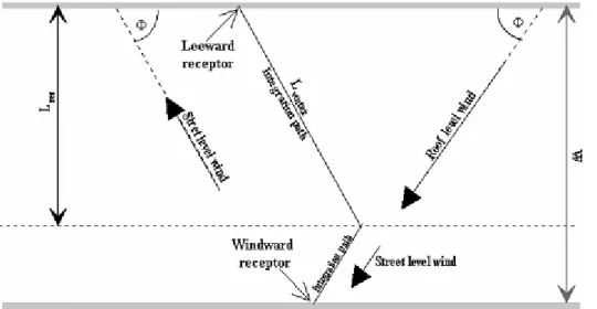
Calculation of the direct flow of pollutants in OSPM is based on the assumption that both the traffic and traffic emissions are uniformly distributed across the canyon. The emission field is treated as a number of infinitesimal line sources, with thickness dx, that are aligned perpendicular to the wind direction at street level. Inside the circulation zone, the wind direction at the street level is assumed to be mirror reflected with respect to the roof level wind. Outside the circulation zone, the wind direction is the same as that at roof level (Figure 2.2).

Figure 2.2 Illustration of the wind flow and formation of the recirculation zone in a street canyon (top view).

dx

W

Q

dQ

=

*

Q is the emission in the street (g m-1 s-1) ; W is the width (m) of the street canyon;

dx (m) is the line perpendicular to the street axis.

The contribution to the concentration at a point located at a distance x from the line source is given by:

)

(

*

*

2

x

u

dQ

dC

=

_π

_σ

ub is the wind speed at the street level;

σz(x) is the vertical dispersion parameter at a downwind distance x. Equation (2.2) is integrated along the wind path at the street level.

Calculation of the vertical dispersion parameter σz in OSPM is based on the assumption that the dispersion of the plume is solely governed by the mechanical turbulence, which is considered to be generated by two mechanisms: the wind and the traffic in the street.

Recirculation contribution:

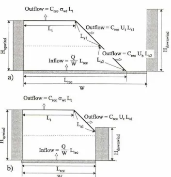
Figure 2.3 Geometry of the recirculation zone. a) The recirculation zone is totally inside the canyon; b) the downwind building intercepts the recirculation zone.

The contribution from the recirculation part of OSPM is calculated assuming a simple box model, which is illustrated in Figure 2.3. The canyon vortex is considered to have a specific shape (see Figure 2.3), with the maximum length of the upper edge being half that of the vortex Lvortex. The ventilation of the recirculation zone takes place through the side of the vortex region, but the ventilation can be limited by the presence of a downwind building if the building intercepts one of the edges (Figure 2.3b).

The length of the vortex, Lvortex, is assumed to be twice the height of the upwind building, Hupwind. For wind speeds (roof level) of less than 2 m/s, it is assumed that Lvortex decreases linearly with decreasing wind speed. This is consistent with the observations that vortex circulation is not observed at low wind speeds.

The concentration in the recirculation zone is calculated assuming that the inflow rate of the pollutants into the recirculation zone is equal to the outflow rate and that the pollutants are well mixed inside the zone.

If we consider the simple case of the vortex being totally immersed inside the canyon (W/H ≤ 1), the recirculation contribution is:

W

Q

C

*

σ

=

σwt is canyon ventilation velocity, which is determined by the turbulence at the top of the canyon. Roughly, σwt ≈ 0.1*ut

where::

ut is the wind speed at the top of the canyon. Chemical processes

Due to the short residence times of air pollutants in street canyons (of the order of seconds or minutes at the most), only the fastest chemical reactions can have any significant influence on the transformation processes in the street canyon air. Therefore, it is assumed in OSPM that only three reactions are of interest:

2 2 3

NO

O

O

NO

₊

_⎯

_⎯→

₊

+

⎯→

⎯

+

h

NO

O

NO

ν

O

O

O

+

→

The reaction between the oxygen radical (O•) and the molecular oxygen (O2) is very fast, and for all practical purposes, the above reaction system can be restricted to two reactions only1_:

- production of NO2 due to the reaction of nitric oxide (NO) with ozone (O3); reaction coefficient: k, ppb-1 s-1 = 5.38e-2*Exp(-1430/T), with T: temperature, Kelvin

- photodissociation of NO2 leading to reproduction of NO and O3; reaction coefficient: J,s-1 = 0.8e-3*Exp(-10/Q) + 7.4e-6*Q, with Q: radiation, W/m2

Assuming that a steady state is achieved within the residence time (time derivates become zero), the NO2 concentration in the street canyon can be calculated as follows (Hertel et al., 1997):

[NO2] = 0.5*(B-(B2-4([NOx]*[NO2]o + [NO2]n*D))1/2) (2.4) where:

[NO2]n = [NO2]v + [NO2]b , with [NO2]v: emitted NO2 and [NO2]v = f* NOx street increment [NO2]o = [NO2]n + [O3]b

B = [NOx] + [NO2]o + R + D where:

R is the photochemical equilibrium coefficient and is given by R=J/k (ppb);

D is the exchange rate coefficient and is equal to (kτ)-1, with τ being the residence time of pollutants in the canyon.

Remark:

In this study, we also performed additional calculations using a method derived from the Dutch model. For convenience, this method is referred to here as “the Dutch method”; it calculates the street increment of NO2 as follows:

100

*

)

1

(

*

)

1

(

*

*

−

+

−

+

=

dNO

f

dNO

f

O

dNO

f

dNO

dNO2, dNOx are the street increments of NO2 and NOx , respectively (in µg/m3); f is the fraction of emitted NO2.

The original Dutch method is also used to calculate the annual average concentration of NO2, and during this operation, it contains a factor 0.6 in the numerator.

2.3

Input and output

- Street configuration (street geometry): average height of buildings, and width and orientation of the street;

- Traffic data: variation in traffic flow over time, categorized into various types of vehicles. It is possible to use the pre-defined traffic data or to specify user-provided traffic data containing the number of various vehicles per hour. Here, we used traffic data provided for two composite vehicles types: “light” and “heavy”. The “light vehicles” category consists of all passenger cars, motor and taxis; the “heavy vehicles” category, all types/sizes of trucks and buses; - Emission data (car fleet and fuel). By default the emission data are calculated based on the

European Emission Model COPERT. However, it is possible to use emission data provided by the user;

- Hourly meteorological data: wind speed, wind direction, radiation, temperature; - Hourly urban background concentration of calculated pollutants;

- For the purpose of the NO2 calculation, the urban background concentration of NO2, NOx and O3 and the percentage of emitted NO2 are also needed.

Output

By default, the results of WinOSPM are summarized in a table where it is possible to compare the model results with air quality limit values. As a supplement to this summary table, it is possible to create a file with an hourly time series and also to create a file with various statistical parameters or daily averages. In this study, we only used the hourly time series.

Comparison between the inputs required by OSPM and those required by the CAR model

OSPM requires both more and more detailed input data than the CAR II model. The major differences between these two models are:

- Street configuration (street geometry): In the OSPM, the street configuration can be given in more detail, with the possibility of defining up to 12 blocks of buildings (and/or open areas) of various heights. However, it is not possible to include the effect of trees in the street in the OSPM. In contrast, in the CAR model, the presence of trees can be compensated for by a factor (the so-called “bomenfactor”). In the OSPM, the monitoring station is assumed to be positioned against the buildings; such positioning is not always the case in the Dutch monitoring network. In the CAR model, such variations in positioning do not represent a problem as the distance between the street axis and the monitoring station is specified in the calculation.

- Traffic and emission data: only average daily data are required by CAR, while average hourly data for working days and for the weekends are required by OSPM.

- Meteorological data: only the yearly average wind speed is required by CAR, while hourly data are required by OSPM. In addition to wind speed data, OSPM also requires data on the wind direction, radiation and temperature.

- Background concentrations: only yearly average concentrations are required by CAR, while hourly data are required by OSPM.

3

Experimental site

3.1

Street configuration

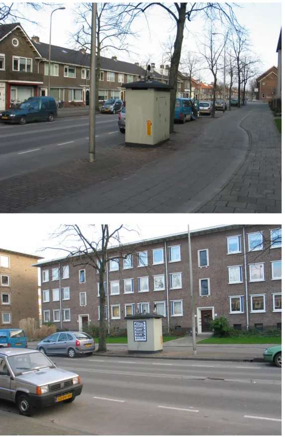
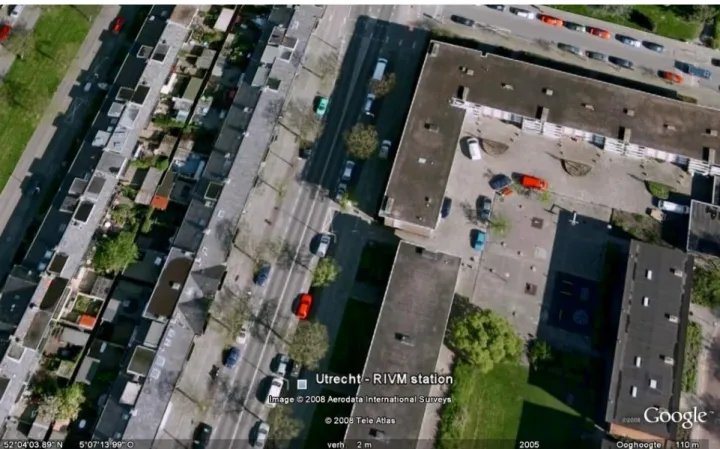
The Erzeijstraat is an urban street with an (almost) continuous line of buildings on both sides (width = 30 m; H = 11 m on the east side and H = 7 m on the west side). The monitoring station is located on the east side of the street, just at the edge of the road surface but off the street itself. Because the distance from the buildings to the monitoring station is approximately 10 m, W = 20 m was used in the standard calculations carried out in this study (the effect of this setting was determined by additional calculations where W was set at 30 m). The street is oriented 16˚ with respect to north. On the south side, 150 m from the monitoring station, is a crossing with more traffic. On the north side, 75 m from the monitoring station, the street becomes more open and is not longer considered to be a street canyon. The developers of OSPM recommend not using length values greater than 75 m, even if the distance is larger; consequently, the model has been run with both L1 and L2 = 75 m (the effect of this setting was determined by additional calculations in which L2 = 150 m was used).

This results in the following street configuration of Erzeijstraat (Figure 3.1) in the standard OSPM calculations:

3.2

Background concentrations and meteorological data

Only measured concentrations were used in this study. Measured concentrations of station 640 (Utrecht-Universiteitsbibliotheek, an urban background station) were available and used up to and including 2003. Because this station was rendered non-operational after 2003, data obtained from the Cabauw measurement station were used for subsequent years. However, this station is a rural monitoring station. The differences between the data obtained from these two stations were determined for the period 1997–2003, resulting in the following correction factors (for more details, see Appendix 1):

NOx_bg = NOx_Cabauw*1.44 NO2_bg = NO2_Cabauw*1.41 O3_bg = O3_Cabauw*0.887

Note: another approach using hourly concentrations (Mooibroek and Wesseling, 2008) results in a different relationship: NOx_Utrecht-Universiteitsbibliotheek = NOx_Cabauw*1.33+3.52. However, these two approaches give comparable results.

Meteological data:

Because Schiphol was used as the reference station in the CAR II model for the area of Utrecht, we also used the measurements recorded at this station as reference values in the present study. The wind speed was corrected for the difference in roughness between the reference station (Schiphol) and the street using the method applied in the Netherlands to calculate the wind speed in urban areas (“Luchtverontreinigingen en weer”, Staatsdrukkerij, 1979). The roughness of Schiphol and the Erzeijstraat was assumed to be 0.08 and 1.5, respectively, resulting in a correction factor of 0.7, id est: u_Erzeijstraat = u_Schiphol*0.7

where:

u is the wind speed (m/s).

All other meteorological data obtained from the Schiphol measurement station (temperature, radiation) were used as obtained, without correction.

To check the effect of meteorological data, we also performed additional calculations using the meteorological data recorded by the Cabauw measurement station.

3.3

Traffic and emission data

Traffic data

Two different sets of traffic data were used in this study.

One set consists of the so-called “old traffic data” and is based, as starting point, on a traffic volume of 9,800 vehicles/weekday, determined in 2003. Specific ratios between various vehicle types were assumed for the weekends and working days, respectively (for more details, see Appendix 2), and the Dutch reference diurnal variation of various vehicles types (Appendix 2) was used.

The second set consists of “new traffic data” and is based on a traffic count performed by the city of Utrecht in 2006 (e-mail on 09/04/2008 from Peter Segaar). This traffic count of vehicles (passenger cars, motors, light trucks, heavy trucks and buses) travelling on the Erzeijstraat was carried out between 0700 and 1900 hours on a working day. The daily volume of each category of vehicles was assumed to be 1.2736 times the traffic volume during this daytime period (with the exception of buses, for which the factor is 1). The reference diurnal profile (Appendix 2) was used to determine the distribution of traffic during the night time. The traffic flows were then categorized into three groups:

- motors and passenger cars were placed into the group ”Passenger cars”; - all buses and light trucks were placed into the group “Light trucks”; - the group “Heavy trucks”.

This results in the following numbers for 2006:

Passenger cars: 10437 vehicles/day

Light trucks: 318 vehicles/day

Heavy trucks: 129 vehicles/day

Total: 10885 vehicles/day

There is no traffic count available for the weekends. However, because a lot of events take place in this area during the weekends and there are many shopping locations in the area itself or close by, the amount of traffic during weekends was assumed to be the same as that on a working day. To calculate the traffic data in a year other than the base year, we assumed that the traffic has increased each year by 2.5%.

Emission data

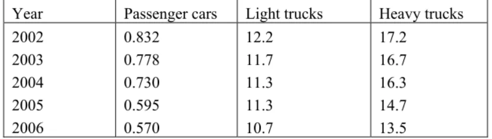
The emission data were calculated using the Dutch reference emission factors taken from the CAR II manual. These are shown in Table 3.1.

Table 3.1: Emission factors of NOx (g/km) used in the present study.

Year Passenger cars Light trucks Heavy trucks

2002 2003 2004 2005 2006 0.832 0.778 0.730 0.595 0.570 12.2 11.7 11.3 11.3 10.7 17.2 16.7 16.3 14.7 13.5

To compensate for the reduced dispersion of pollutants due to the presence of trees in this street, the emissions were multiplied by 1.5 (the so-called “bomenfactor”).

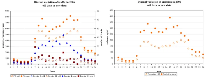
Note: Although it is more logical to apply this bomenfactor to the residence time of the pollutants, this option is not possible with the current version of OSPM. Because a reduced dispersion results in a higher concentration of pollutants, we simulated the effect in this study by changing the emission. An example of the emission calculation is shown in Appendix 3. The 2006 traffic and emission data are presented in Figures 3.4 and 3.5, respectively.

Diurnal variation of emission in 2006 old data vs new data

0 50 100 150 200 250 300 350 400 450 0 1 2 3 4 5 6 7 8 9 10 11 12 13 14 15 16 17 18 19 20 21 22 23 24 hour emi ss io n , µ g/m 3

Emission, old Emission, new

Diurnal variation of traffic in 2006 old data vs new data

0 100 200 300 400 500 600 700 800 900 0 1 2 3 4 5 6 7 8 9 10 11 12 13 14 15 16 17 18 19 20 21 22 23 24 hour nu mber of p as senger cars 0 10 20 30 40 50 60 n um be r o f t ruc ks

PA,old PA,new Trucks_L,old Trucks_H, old Trucks_L,new Trucks_H, new

Figure 3.4: Diurnal variation of traffic and emissions on working days in Erzeijstraat according to the “new” and “old” traffic data sets, respectively. The daily average emissions are 219.4 µg/m/s (old) and 193 µg/m/s (new).

Diurnal variation of emission in 2006 old data vs new data

0 50 100 150 200 250 300 350 400 450 0 1 2 3 4 5 6 7 8 9 10 11 12 13 14 15 16 17 18 19 20 21 22 23 24 hour em is si on , µg /m 3

Emission, old Emission, new

Diurnal variation of traffic in 2006 old data vs new data

0 100 200 300 400 500 600 700 800 900 0 1 2 3 4 5 6 7 8 9 10 11 12 13 14 15 16 17 18 19 20 21 22 23 24 hour nu m be r o f p asse nge r c ar s 0 10 20 30 40 50 60 nu m be r o f t ruc k s

PA,old PA,new Trucks_L,old Trucks_H, old Trucks_L,new Trucks_H, new

Figure 3.5: Diurnal variation of traffic and emission during weekends in Erzeijstraat according to the “new” and “old” traffic data sets, respectively. The daily average emissions are 111.5 µg/m/s (old) and 193 µg/m/s (new).

It must be noted that the traffic count in 2006 shows that the traffic in the Erzeijstraat is not symmetrical.

The traffic count in Erzeijstraat in 2006 is shown in Figure 3.6.

Erzeijstraat 2006 0 50 100 150 200 250 300 350 400 450 500 0700-0800 0800-0900 0900-1000 1000-1100 1100-1200 1200-1300 1300-1400 1400-1500 1500-1600 1600-1700 1700-1800 1800-1900 hr n u m b ers P A 0 5 10 15 20 25 30 35 40 45 50 n um be rs he av y dut y

PA,North PA,South heavy duty,North heavy duty,South

Figure 3.6: Diurnal variation of traffic in Erzeijstraat in the northerly and southerly direction, respectively. PA = motors + passenger cars + taxis; heavy duty = buses + all types/sizes of trucks.

3.4

Performed calculations

The following calculations were performed: Year Street

configuration

Meteorological station used

Background station Traffic data Purpose 2002 &

2003

Standard (*) Schiphol

Utrecht-Universiteitsbibliotheek (LML640)

Both traffic data (old and new) were used

Standard runs. Also to determine the effect of the traffic data used

2002 Standard (*) Schiphol

Utrecht-Universiteitsbibliotheek Alternative profile (**) Determine the effect of the traffic data used

2002 W=30 m Schiphol

Utrecht-Universiteitsbibliotheek

new Determine the

effect of setting in OSPM

2002 L2=150 m Schiphol

Utrecht-Universiteitsbibliotheek

new Determine the

effect of the settings in OSPM

2006 Standard (*) Schiphol Cabauw

(LML620)

new Determine the

effect of the background data used

2006 Standard (*) Cabauw Cabauw new Determine the

effect of the meteorological data used (*): Standard street configuration means: L1 = L2 = 75 m; W = 20 m

(**): Based on the assumption that the traffic volume is equal to twofold that of the traffic travelling in the northerly direction

4

Comparison with measurements

4.1

Method

The model results were evaluated both graphically (plotting of model results against observed data) and statistically. The following statistical parameters were used in this study:

- Mean: arithmetic mean - Bias: observed – modelled - Sigma: standard deviation

- Cor: correlation between the observed and modelled values (good correlation: R value of 0.9 or higher)

- MSSE (Mean Square of Standard Error), defined as: MSSE= 1 _{*∑ (Model−Observation)}2

N

Only hourly concentrations for which both measured and modelled values are available, were used. Data with wind direction 0 (defined as variable wind direction) were not used.

4.2

Results of standard calculations for 2002 and 2003

The results obtained for 2002 and 2003 are presented in Table 4.1. The calculations were performed for both sets of traffic data (new and old), and comparisons with measurements were done for all days as well as for working days only. The results of the calculations for 2002 are shown graphically in the Figures 4.1–4.4. To investigate if the correlation improves when the extremes are removed, we also plotted the results for measured NOx concentrations below 400 and 200 µg/m3, respectively (Figure 4.2).

Table 4.1: Comparison between modelled and measured NOx concentrations and street increments

(dNOx) in the Erzeijstraat. Concentrations are given in µg/m3. Street configuration used: L1 = L2 = 75 m, W = 20 m.

All days Working days All days Working days All days Working days All days Working days

Data points 6620 4674 6620 4674 6727 4778 6727 4778 Mean_bg 50.0 54.3 50.0 54.3 50.5 56.9 50.5 56.9 Mean_obs 101.0 110.7 101.0 110.7 105.4 118.4 105.4 118.4 Mean_mod 109.1 113.2 108.5 121.5 110.6 116.3 110.0 124.8 Bias -8.0 -2.4 -7.5 -10.8 -5.2 2.1 -4.6 -6.3 Sigma_obs 96.1 102.2 96.1 102.2 114.9 127.8 114.9 127.8 Sigma_mod 77.5 80.3 80.2 84.5 79.6 86.8 83.4 91.0 Cor_total_NOx 0.85 0.88 0.87 0.88 0.85 0.88 0.87 0.88 MSSE 50.9 49.7 48.1 50.8 63.8 66.0 60.0 65.1 Cor_dNOx 0.63 0.64 0.58 0.60

2002, new traffic data 2002, old traffic data 2003, new traffic data 2003, old traffic data

Abbreviations:

Mean_bg: average background concentration;

Mean_obs, mean_mod: average of measured concentrations and modelled concentrations, respectively; Bias: difference between measured and modelled values;

Sigma_obs, sigma_mod: Standard deviation of measured and modelled concentrations, respectively; Cor_total_NOx: Correlation coefficient between measured and modelled total NOx concentrations;

MSSE: Mean Square of Standard Error, as defined above;

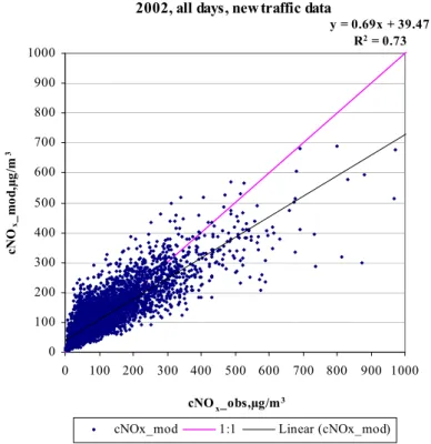
2002, all days, new traffic data y = 0.69x + 39.47 R2 _{= 0.73} 0 100 200 300 400 500 600 700 800 900 1000 0 100 200 300 400 500 600 700 800 900 1000 cNO_x_obs,µg/m3 cNO x _m od ,µ g/ m 3

cNOx_mod 1:1 Linear (cNOx_mod) 2002, working days, new traffic data

y = 0.69x + 36.69 R2 _{= 0.77} 0 100 200 300 400 500 600 700 800 900 1000 0 100 200 300 400 500 600 700 800 900 1000 cNO_x_obs,µg/m3 cN Ox _m od ,µ g/ m 3

cNOx_mod 1:1 Linear (cNOx_mod)

Figure 4.1: Comparison between modelled and measured total NOx concentrations in 2002 using the new

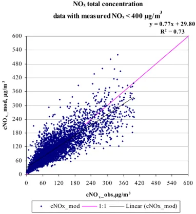
NOx total concentration data with measured NOx < 400 µg/m3

y = 0.77x + 29.80 R2 _{= 0.73} 0 60 120 180 240 300 360 420 480 540 600 0 60 120 180 240 300 360 420 480 540 600 cNO_x_obs,µg/m3 cNO x _m od , µ g/ m 3

cNOx_mod 1:1 Linear (cNOx_mod) NOx total concentration

data with measured NOx < 200 µg/m3

y = 0.85x + 23.69 R2 _{= 0.63} 0 40 80 120 160 200 240 280 320 360 400 0 40 80 120 160 200 240 280 320 360 400 cNO_x_obs, µg/m3 cNO x _m od , µ g/ m 3

cNOx_mod 1:1 Linear (cNOx_mod)

Figure 4.2: Performance of the model for various ranges of measured NOx concentrations in 2002 using

the new traffic data set and working days only. Upper: Model results for measured total NOx concentration

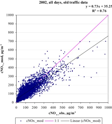
2002, all days, old traffic data y = 0.73x + 35.25 R2 _{= 0.76} 0 100 200 300 400 500 600 700 800 900 1000 0 100 200 300 400 500 600 700 800 900 1000 cNOx_obs, µg/m3 cNO x _m od , µ g/ m 3

cNOx_mod 1:1 Linear (cNOx_mod)

2002, working days, old traffic data

y = 0.72x + 41.30 R2 _{= 0.77} 0 100 200 300 400 500 600 700 800 900 1000 0 100 200 300 400 500 600 700 800 900 1000 cNOx_obs, µg/m3 cN Ox _m od , µ g/ m 3

cNOX_mod 1:1 Linear (cNOX_mod)

Figure 4.3: Comparison between modelled and measured total NOx concentrations in 2002 using the old

traffic data set. Upper: All days. Below: Working days only. Note that the model results are improved with the old traffic data set also when the weekends are not included.

2002, workingdays, new traffic data y = 0.44x + 34.28 R2 _{= 0.39} 0 50 100 150 200 250 300 350 400 450 500 -50 0 50 100 150 200 250 300 350 400 450 500 dNO_x_obs, µg/m3 dN Ox _m od , µ g/ m ³

dNOx_mod 1:1 Linear (dNOx_mod)

Figure 4.4: Comparison between modelled and measured NOx street increments in 2002 using the new

traffic data set. Only data for working days were used. Effect of traffic data

The results in Table 4.1 show a good correlation between the measured and the modelled NOx concentrations (R = 0.88) and a moderate correlation for the street increment (R = 0.63). Measured concentrations have much larger standard deviation (sigma) than modelled values, indicating that the extremes can not be predicted well by the model. The linear (least square) regression lines have intercepts of about 40 µg/m3 (Figures 4.1 and 4.3) and slopes of about 0.7. Lower intercepts and higher slopes were obtained when only measured data below 400 µg/m3 and 200 µg/m3, respectively, were used (Figure 4.2).

Comparisons between the results obtained with the two sets of traffic data show that:

- Both sets of traffic data lead to an overestimation of the average concentration (negative bias). - When only data for working days are used, modelling with the new traffic data set results in an

average NOx concentration that is quite close to the measured values (bias ± 2 µg/m3). The emissions obtained with the old set of traffic data are about 13% higher than those obtained with the new data set (see Figure 3.4), resulting in the same increase in the street increment and a higher bias.

- The new traffic data set assumes that the traffic during the weekends is the same as that during working days. This assumption leads to a large overestimation of the weekend’s emissions; consequently, when the data for the weekends are included, the bias becomes more negative. Figure 4.4 shows that there is an undesirable effect of using background concentrations measured at a location other than the monitoring site. Although the yearly average concentrations measured at the Utrecht-Universiteitsbibliotheek station were lower than those of the Erzeijstraat, the hourly concentrations at the former location could, on occasion, actually be higher than those at the latter location, as can be seen in Figure 4.4 (negative value for observed street increment). This variation causes a discrepancy between the model results and observations. In Jagtvej (Copenhagen, Denmark), where OSPM has been tested successfully, the background concentration was obtained at a monitoring station located at the experimental site, but at a height of 20 m.

Overall, we can conclude that the new set of traffic data gives slightly better results – provided that the incorrect data for the weekends are not used (id est the seemingly incorrect assumption that traffic during the weekends is the same as that on working days). This is also shown in Figure 4.5, which depicts the diurnal variation of NOx concentration for both sets of traffic data. Figure 4.5 also shows the effect of traffic on the background station Utrecht–Universiteitsbibliotheek: the background concentration is much higher on working days than during weekends, with a difference of almost 50 µg/m3 during peak hours.

Diurnal variation of NOx in Erzeijstraat

2002, working days , new vs old traffic data

0 50 100 150 200 250 0 2 4 6 8 10 12 14 16 18 20 22 24 hr cN Ox ,µg/ m 3

Average of cNO x_bg Average of cNO x_obs

Average of cNO x_mod_new data Average of cNO x_mod_old data

Diurnal variation of NOx in Erzeijstraat

2002, weekends , new vs old traffic data

0 50 100 150 200 250 0 2 4 6 8 10 12 14 16 18 20 22 24 hr cN Ox ,µg/ m 3

Average of cNO x_bg Average of cNO x_obs

Average of cNO x_mod_new data Average of cNO x_mod_old data

Figure 4.5: Modelled and measured diurnal variations of NOx. Upper: working days only. Below: weekends

only. Both sets of traffic data lead to an overestimation of the concentrations, but the overestimation of the old data set is larger. The new traffic data set strongly overestimates the concentrations during the weekends.

An additional calculation was performed using a modified profile of the new traffic data set. In this calculation the traffic is assumed to be twice that of traffic travelling in the northerly direction. Because the new set of traffic data already overestimates the average concentrations (negative bias), the bias became even more negative when the modified set of traffic data was used. No effect on the correlation was observed.

The result of this calculation is shown in Table 4.2 and Figure 4.6.

Table 4.2.: Comparison between modelled and measured NOx concentrations: new traffic data versus

modified traffic profile. The calculation was performed with data for 2002; only working days were used.

Standard Traffic=2* north direction

Data points 4674 4674 Mean_bg 54.3 54.3 Mean_obs 110.7 110.7 Mean_mod 113.2 116.2 Bias -2.4 -5.5 Sigma_obs 102.2 102.2 Sigma_mod 80.3 82.0 Cor_total_NOx 0.88 0.88 MSSE 49.7 50.0 Cor_dNOx 0.63 0.63

Diurnal variation of NOx in Erzeijstraat

2002, working days 0 50 100 150 200 250 0 2 4 6 8 10 12 14 16 18 20 22 24 hr cN O x ,µg/ m 3

Average of cNO x_bg Average of cNO x_obs

Average of cNO x_mod_new data Average of cNO x_mod_2*traffic north direction

Figure 4.6: Diurnal variation in modelled and measured NOx concentrations: new traffic data versus

Effect of wind directions

Figure 4.7 shows the NOx concentration as a function of wind directions for 2002. It is evident from this figure that the model makes a large underestimation (up to almost half of the street increment) when the wind is in a southeasterly direction. One possible explanation for this result may be the contribution of the large and crowded intersections located at the southern end of the Erzeijstraat. There are also significant highway emissions roughly 1 km south and roughly 2 km southeast of the Erzeijstraat. However, when the data associated with the southeasterly wind (wind sectors between and including 130–170˚) were left out, the results did not improve because the model then overestimated the average concentration (Figure 4.8 versus Figure 4.5); The correlation between the modelled and measured NOx concentrations was also not improved (Table 4.3)

NOx concentration in Erzeijstraat as a function of wind directions Year 2002, new traffic data, all wind directions

0 50 100 150 200 250 0 30 60 90 120 150 180 210 240 270 300 330 360 wind direction cN O x , µ g/ m 3

Average of cNO x_bg Average of cNO x_obs Average of cNO x_mod

Diurnal variation of NOx in Erzeijstraat

2002, working days , without southeasterly wind

0 50 100 150 200 0 2 4 6 8 10 12 14 16 18 20 22 24 hr cN Ox ,µ g/ m 3

Average of cNO x_mod, new traffic data Average of cNO x_obs

Average of cNO x_bg Average of cNO x_mod, old traffic data

Figure 4.8: Diurnal variations in total NOx concentrations on working days. The data for southeasterly

winds are not included.

Table 4.3. Average total NOx concentrations and correlations between modelled and measured data.

Results of 2002 for new traffic data set and for working days only.

Hour Mean_bg Mean_obs Mean _mod Bias Cor_NOx Mean_bg Mean_obsMean _mod Bias Cor_NOx

1 43.2 66.4 66.9 -0.5 0.88 45.9 72.3 69.9 2.4 0.89 2 38.6 50.6 56.6 -6.0 0.97 41.2 55.7 59.6 -3.9 0.96 3 35.6 45.3 48.1 -2.8 0.97 37.8 50.0 50.6 -0.6 0.96 4 28.4 35.9 41.6 -5.8 0.90 31.3 40.6 44.6 -4.0 0.93 5 29.5 38.2 42.1 -3.9 0.94 33.5 45.6 46.3 -0.6 0.94 6 31.0 54.3 59.0 -4.8 0.88 35.4 65.8 64.2 1.6 0.88 7 47.6 114.4 139.1 -24.7 0.81 51.4 134.7 146.3 -11.6 0.78 8 71.1 163.6 161.6 2.0 0.81 77.3 195.7 172.7 23.0 0.84 9 74.6 153.7 175.7 -21.9 0.80 84.2 188.4 191.2 -2.8 0.80 10 75.7 153.1 158.8 -5.7 0.90 80.5 168.6 166.0 2.6 0.90 11 64.2 127.6 151.4 -23.9 0.86 70.6 148.2 161.8 -13.6 0.88 12 56.0 112.3 131.1 -18.8 0.80 60.7 127.7 140.1 -12.4 0.84 13 49.1 100.0 115.8 -15.8 0.84 53.6 115.5 125.6 -10.1 0.88 14 48.4 105.0 123.0 -18.0 0.78 52.2 117.5 131.6 -14.0 0.85 15 46.5 98.8 137.0 -38.2 0.75 51.0 113.3 147.9 -34.6 0.81 16 46.0 108.9 119.8 -10.9 0.82 50.6 122.8 129.5 -6.7 0.86 17 47.4 105.2 129.5 -24.3 0.85 52.8 119.1 138.3 -19.2 0.88 18 48.6 98.6 113.1 -14.4 0.87 56.2 117.1 125.7 -8.6 0.90 19 51.0 106.0 113.9 -7.9 0.88 54.8 117.5 119.6 -2.2 0.89 20 51.2 103.4 106.2 -2.8 0.90 56.7 116.0 114.0 1.9 0.92 21 50.8 98.6 89.3 9.3 0.91 55.3 107.9 95.2 12.8 0.91 22 52.3 98.2 88.1 10.1 0.91 56.5 107.6 93.3 14.3 0.92 23 49.7 96.2 87.5 8.8 0.88 55.5 108.4 94.2 14.2 0.90

Effect of wind speed

To determine the effect of wind speed on the model performance, the data for 2002 were divided into two groups: data with wind speeds ≥ 3 m/s and data with lower wind speeds. The results are presented in Table 4.4. As expected, the concentrations are lower at higher wind speeds. The results also suggest that the model performs better at higher wind speeds (better correlation of the street increment). However, a lower wind speed mostly occurs in the Erzeijstraat when the wind is in a southeasterly direction (Figure 4.9). This is precisely the situation in which the contribution from the intersections and highways lying to the south of the Erzeijstraat may be quite pronounced – and the situation which can not be reproduced by the model. Therefore, in this case, it is not possible to draw any conclusion on the effect of wind speed on the performance of the model.

Table 4.4: Dependence of model results on wind speed. Results for 2002, the new set of traffic data and only data for working days were used. Reported wind speeds are over the roof level (the so-called “u_mast”in OSPM).

all wind speeds ws ≥ 3 m/s ws < 3 m/s

Data points 4674 2483 2191 Mean_bg 54.3 40.5 69.9 Mean_obs 110.7 81.7 143.7 Mean_mod 113.2 86.7 143.2 Bias -2.4 -5.0 0.5 Cor_total_NOx 0.88 0.88 0.86 MSSE 49.7 28.4 66.0 Mean_dNOx_obs 56.5 41.2 73.8 Mean_dNOx_mod 58.9 46.2 73.3 Cor_dNOx 0.63 0.73 0.55

Street increment of NOx as a function of wind directions

0 30 60 90 120 150 0 30 60 90 120 150 180 210 240 270 300 330 360 wind direction dN Ox , µg/ m 3 0 1 2 3 4 5 6 7 8 9 10 w in d s p eed , m /s

Average of dNO x_obs Average of dNO x_mod

Average of wind speed

Effect of the “bomenfactor”

In this study, the emissions were multiplied by 1.5 to simulate the effect of trees in the Erzeijstraat. No distinction was made between the summer and the winter periods. We investigated the effect of the introduction of a constant factor for the whole year. The results are shown in Figures 4.10A, B, C on a per-month basis for 2002, 2003 and 2006, respectively. Theoretically, the effect of trees is more significant during the summer period, and the model should underestimate the results; in contrast, the model should overestimate the effect of trees during the winter periods.

However, Figure 4.10A–C shows that the model overestimates the “bomenfactor” even during June, July and August. One explanation for this unexpected result may be the numerous legal holidays that occur during this period: the reduction in the amount traffic on these days may have a larger effect than the overgrowth of trees.

In 2002 and 2006, the model does make relatively more overestimations during the winter period than in other months (provided that the holiday period is left out of the calculation). This effect is, however, not observed in 2003.

Erzeijstraat, 2002, new traffic data

0 50 100 150 200 1 2 3 4 5 6 7 8 9 10 11 12 month cNO x , µ g/ m 3

Average of cNOx_obs_2 Average of cNOx_b Average of cNOx_mod_2

Figure 4.10A: Monthly average of total NOx concentrations: Model versus observation for working days of

2002. No data are available for October because the background concentration is missing. The black arrows show the “winter period” (period without any overgrowth of trees).

Erzeijstraat, 2003, new traffic data 0 50 100 150 200 250 300 1 2 3 4 5 6 7 8 9 10 11 12 month cNO x , µ g/ m 3

Average of cNOx_obs_2 Average of cNOx_b Average of cNOx_mod_2

Figure 4.10B: Monthly average of total NOx concentrations: Model versus observation for working days of

2003. The black arrows show the winter period.

Erzeijstraat, 2006, new traffic data

0 50 100 150 200 250 1 2 3 4 5 6 7 8 9 10 11 12 month cNO x , µ g/ m 3

Average of cNOx_obs_2 Average of cNOx_b Average of cNOx_mod_2

Figure 4.10C: Monthly average of total NOx concentrations: Model versus observation for working days of

4.3

Additional calculations performed for 2002: effect of various settings in

OSPM

In previous calculations the street configuration was set at L1 = L2 = 75 m and W = 20 m. We have carried out a number of additional calculations aimed at investigating the effect of the street configuration on the modelled concentrations:

- The actual length of the Erzeijstraat (L2 = 150 m) was used in one calculation. (id est ignoring the recommendation of OSPM not to define a length > 75 m).

- The actual width of Erzeijstraat (W = 30 m) was used in a second calculation (id est without taking into account the fact that the monitoring station is located about 10 m away from the buildings).

Table 4.5: Effect of the street configuration on the average NOx concentration and on the correlation

between model and measurements. Data of 2002, new traffic data set and working days only.

Standard L2 = 150 m W = 30 m Data points 4674 4674 4674 Mean_bg 54.3 54.3 54.3 Mean_obs 110.7 110.7 110.7 Mean_mod 113.2 114.5 102.4 Bias -2.4 -3.7 8.3 Sigma_obs 102.2 102.2 102.2 Sigma_mod 80.3 80.9 72.4 Cor_total_NOx 0.88 0.88 0.88 MSSE 49.7 49.9 52.1 Cor_dNOx 0.63 0.63 0.59

As expected, the modelled concentration decreases when the width of the street increases from 20 m to 30 m. Using the standard setting, the modelled values are 2.4 µg/m3 _{higher than the measurements;} with W = 30 m, the modelled values are 8.3 µg/m3 lower than the measurements. However, despite this noticeable effect on the average concentration, the effect on the correlation (R) is negligible.

When the length of the street is increased from 75 m to 150 m, the average concentration increases slightly (1.3 µg/m3_{). There is no observed effect on the correlation.}

4.4

Calculations performed for 2006

The results obtained for 2006 are presented in Table 4.6. The calculations were performed using data obtained from the LML station at Cabauw as background values. The NOx concentration recorded at the Cabauw measurement station was then multiplied by 1.44 to compensate for the (average) difference between this station and the Utrecht-Universiteitsbibliotheek station (see also Appendix 1). To test the effect of the meteorological data, we performed the calculations using meteorological data obtained from both the Cabauw and Schiphol locations.

The roughness of these locations is shown in Appendix 4. At first glance, there is no substantial difference between the roughness of the Cabauw and Schiphol locations. The roughness lengths of Schiphol and the Erzeijstraat are assumed to be 0.08 m and 1.5 m, respectively. If a roughness length of 0.1 m is assumed for Cabauw, the corresponding correction factors for these two locations are 0.705 (Schiphol) and 0.714 (Cabauw), which are more or less the same. We therefore applied a correction factor of 0.7 for both stations in this study.

The results presented in Table 4.6 show that both the bias and the correlation coefficient obtained for 2006 are worse than those for 2002 and 2003. When the Schiphol data were used, the modelled street increment is approximately 5 µg/m3 lower than when the Cabauw data were used. This result can be explained by the higher wind speed at Schiphol relative to Cabauw (annual average wind speeds were 5 m/s and 4.3 m/s, respectively). Because the same correction factor was applied, these calculations were therefore performed with different wind speeds. The higher wind speed of the Schiphol data set results in an approximately 10% lower street increment.

For 2006, the results obtained using the meteorological data from Schiphol are slightly better than those obtained using the data from Cabauw.

Table 4.6: Comparison between modelled and measured NOx concentration and the street increment

Calculations were performed with the new traffic data set. The results are for working days only.

2002_Schiphol 2003_Schiphol 2006_Schiphol 2006_Cabauw

Data points 4674 4778 5694 5651 Mean_bg 54.3 56.9 48.5 49.0 Mean_obs 110.7 118.4 92.8 93.9 Mean_mod 113.2 116.3 97.3 103.3 Bias -2.4 2.1 -4.5 -9.4 Sigma_obs 102.2 127.8 107.1 109.4 Sigma_mod 80.3 86.8 77.2 79.1 Cor_total_NOx 0.88 0.88 0.77 0.76 MSSE 49.7 66.0 69.0 72.1 Cor_dNOx 0.63 0.58 0.44 0.42

Note: there is small difference between the observed values when meteorological data obtained from Cabauw and Schiphol, respectively, are used. This is due to the fact that data with wind direction 0 are eliminated in this study; therefore, the data sets used in the comparison are not completely the same for Cabauw and Schiphol.

4.5

Performance of the NO

calculation by OSPM

The performance of the OSPM model on the NO2 calculation was determined for 2002 and 2003. Additional calculations performed were:

- NO2 calculations according to the Dutch method;

- NO2 calculations according to the OSPM method (see chapter 2.2), although with modified values of τ (residence time of pollutant in the street canyon). In these calculations, the τ values of OSPM were multiplied by a factor, and these modified τ values were used for calculating

NO2. It is not possible to output the residence time τ in the current version of WinOSPM. We therefore calculated τ outside OSPM using the OSPM method (information from Ketzel, M.; e-mail on 29/05/2008), using H = 11 m. The calculation of τ is described in Appendix 5.

The default factors used by OSPM were used to convert micrograms per cubic metre to parts per billion, and vice versa. These are: 1 µgNO2/m3 = 0.5217 ppb NO2, 1 µgNOx/m3 = 0.5217 ppb NOx and 1 µg O3/m3 = 0.5 ppb O3

The fraction of emitted NO2 in the Netherlands has increased from about 6% in 2000 to 13% in 2006 (Mooibroek and Wesseling, 2008). The following fractions of emitted NO2 were used in this study:

f_NO2 Erzeijstraat 2002 8.7 2003 9.7 2004 10.6 2005 11.5 2006 12.5

(Bold values: years used in the present study) The results are presented in Tables 4.7 and 4.8.

Table 4.7: Comparison between modelled and measured NO2 concentrations and NO2 street increments in

the Erzeijstraat using the new traffic data set. Reported values are based on the data for working days in 2002.

First column: Dutch method, using measured NOx concentrations. The next three columns represent the results obtained using the Dutch method, the OSPM and the OSPM method using modified residence times, which were set at 1.5 times the τ values produced by OSPM. All concentrations are in µg/m3.

Dutch (measured NOx ) Dutch OSPM OSPM_1.5Tau

Mean_bg 35.7 35.7 35.7 35.7 Mean_obs 47.7 47.7 47.7 47.7 Mean_mod 48.0 50.3 46.5 47.7 Bias -0.3 -2.6 1.2 0.0 Sigma_obs 21.6 21.6 21.6 21.6 Sigma_mod 20.8 18.7 18.6 18.7 Cor_total_NO2 0.97 0.85 0.87 0.87 Mean_dNO2_obs 12.1 12.1 12.1 12.1 Mean_dNO2_mod 12.4 14.7 10.8 12.1 Cor_dNO2 0.91 0.62 0.63 0.64

Table 4.8: Comparison between modelled and measured NO2 concentrations: data of 2003

Dutch (measured NOx ) Dutch OSPM OSPM_1.5Tau

Mean_bg 38.4 38.4 38.4 38.4 Mean_obs 52.9 52.9 52.9 52.9 Mean_mod 53.1 55.5 51.0 52.4 Bias -0.2 -2.6 1.9 0.5 Sigma_obs 26.7 26.7 26.7 26.7 Sigma_mod 26.1 22.2 22.4 22.3 Cor_total_NO2 0.97 0.86 0.89 0.89 Mean_dNO2_obs 14.5 14.5 14.5 14.5 Mean_dNO2_mod 14.8 17.1 12.7 14.1 Cor_dNO2 0.90 0.58 0.59 0.59

ite close to the measured values on by about 5%) nd a slightly worse correlation compared to that obtained using the OSPM method.

odelled NO2 concentration is mainly caused by the deviation in the modelled NOx oncentration.

02 are presented in the Figures 4.11– 4.14.

Tables 4.7 and 4.8 show that the default OSPM results have a positive bias (measured values are higher than those of the model), which is about 12% of the street increment. The correlation between the modelled and measured concentration is good (R = 0.87 and 0.89, respectively), but that for the street increment is only moderate (R = 0.59 and 0.63, respectively). When the residence time produced by OSPM was multiplied by 1.5, the average concentrations became qu

(bias close to 0). However, no effect on the correlation was observed.

The Dutch method results in negative bias (overestimation of the average concentrati a

A good correlation was obtained between the calculated and the measured NO2 concentration when the measured NOx concentrations were used in the calculation of NO2. This result indicates that the deviation in the m

c

Erzeijstraat 2002 y = 0.75x + 10.52 R2 _{= 0.77} 0 20 40 60 80 100 120 140 160 0 20 40 60 80 100 120 140 160 NO₂_obs, µg/m3 NO 2 _OS P M , µ g/ m 3

cNO2_OSPM µg/m3 1:1 Linear (cNO2_OSPM µg/m3)

Figure 4.11: Comparison between modelled and measured NO2 concentrations in 2002 using the new

traffic data set. Only data of working days were used.

Erzeijstraat 2002 _{y = 0.75x + 11.73} R2 _{= 0.76} 0 20 40 60 80 100 120 140 160 0 20 40 60 80 100 120 140 160 NO2_obs, µg/m3 NO 2 _O SP M _1. 5 T au , µ g/ m 3

NO2_1.5T au µg/m3 1:1 Linear (NO2_1.5T au µg/m3)

Figure 4.12: Performance of the OSPM method when the residence time used in the NO2 calculation was

Erzeijstraat 2002 y = 0.73x + 15.32 R2 _{= 0.72} 0 20 40 60 80 100 120 140 160 0 20 40 60 80 100 120 140 160 NO2_obs, µg/m3 NO 2 _D ut ch , µ g/ m 3

cNO2_Dutch µg/m3 1:1 Linear (cNO2_Dutch µg/m3)

Figure 4.13: Comparison between the Dutch method and measurements.

Erzeijstraat 2002

NO2 concentration calculated with measured NOx

y = 0.93x + 3.68 R2 _{= 0.93} 0 20 40 60 80 100 120 140 160 0 20 40 60 80 100 120 140 160 NO2_obs, µg/m3 NO 2 _D ut ch , µ g/ m 3

cNO2_Dutch µg/m3 1:1 Linear (cNO2_Dutch µg/m3)

Figure 4.14: Results obtained with the Dutch method when measured NOx concentration was used. Using

the measured NOx concentration for the calculation of NO2 produced a very good correlation between the

5

Discussion

5.1

Quality of used input data

For the OSPM model to perform well, it is essential that the input data (traffic flow, emission data and meteorological data) are accurate. Consequently, the lack of a meteorological station at the experimental site is likely to be an important factor contributing to the observed differences between the modelled results obtained in this study and the measured data. OSPM has been tested extensively in Denmark, where it has proven to be a highly accurate and reliable model for estimating pollution emissions from traffic. Most of the Danish tests were performed using data obtained in Jagtvej, where the meteorological data were recorded on two meteorological masts located at the location itself. It is not yet possible to estimate how much the model results will be improved when detailed local meteorological data are available. The most relevant factor in this context is the wind speed as the street increment is roughly inversely proportional to the wind speed.

Another factor that affects the performance of OSPM is the use of background concentrations measured at a location other than the monitoring site (Dutch situation). Although the yearly average concentrations measured at the Utrecht-Universiteitsbibliotheek station were lower than those obtained for the Erzeijstraat, the hourly concentrations at the Utrecht-Universiteitsbibliotheek can occasionally be higher than those recorded in the Erzeijstraat. As such, this variation also accounts for the discrepancy between the model results and the measurements.

5.2

Erzeijstraat versus Jagtvej

In addition to the better quality of the input data of Jagtvej, as mentioned above, there are a number of other differences between the Jagtvej and Erzeijstraat locations:

The traffic density is much higher in Jagtvej. In 1994, when the model was being tested using the Jagtvej data, the traffic flow in Jagtvej was 22000 vehicles/day; in contrast, in 2006, the traffic flow in Erzeijstraat was only about 11000 vehicles/day. If yearly increases in traffic flow are taken into account, the traffic intensity in Jagtvej is about threefold greater than that of Erzeijstraat (the width of these two streets is comparable).

Furthermore, Jagtvej is flanked on both sides with high buildings (18 m compared to approximately 7–11 m along the Erzeijstraat), which results in a relatively large street increment in Jagtvej compared to that in the Erzeijstraat. In Jagtvej, a large fraction of the total NOx concentration is street increment (information from M. Ketzel), whereas this fraction is substantially smaller in the Erzeijstraat. Small street increments may lead to a poorer correlation between the modelled and observed values (because the observed street increment is the difference between two relatively large values).

5.3

NO

calculation

The NO2 calculations with modified τ show that the modelled values are improved when a larger τ is used for the NO2 calculation. The use of this modification does not necessarily mean that the residence time of the pollutants in Erzeijstraat is longer than that modelled by the OSPM; rather, it may imply that the NO2 reaction kinetic as used in the model OSPM does not represent the Dutch situation very well. This result is not surprising as the reaction constants used by OSPM were determined experimentally in Denmark where the circumstances may different from those found in the Netherlands.

6

Conclusions

The study reported here shows that:

• A good correlation between modelled and measured total NOx concentrations (R = 0.89) can be obtained with the OSPM. The correlation between the modelled and measured street increments is moderate (R = 0.64). The lack of accurate meteorological data and the contribution from the highways and intersections located south of the Erzeijstraat are probably the main factors contributing to the latter.

• The new set of traffic data, which is based on traffic counts performed by the city of Utrecht in 2006, produces much better results for working days than the old set of traffic data (bias of ± 2% for total NOx concentrations compared to a bias of up to –10%, respectively). The new data set assumes that traffic intensity during the weekends is the same as that on working days; this assumption is clearly not valid. Therefore, when data on the weekends are included in the model, the results obtained with the new set of traffic data become worse.

• The OSPM seems to be robust. A small change in the street configuration setting does not result in significant changes in the result

• The correlation between the modelled and measured NO2 concentrations is mainly determined by the quality of the modelled NOx.

• The modelled annual NO2 concentration has a bias of less than 5% of the measured total NO2 concentration, which is comparable to the performance of the CAR II model (Wesseling et al., 2007). The difference between modelled and measured average concentrations can be reduced to almost zero when the τ values produced by OSPM are multiplied by 1.5 before they are used for the NO2 calculations. This results in a larger NOx/NO2 conversion.

• The Dutch method for calculating the NOx/NO2 conversion gives slightly worse results than the OSPM method.

Based on these preliminary results, we recommend that the OSPM be explored in more detail. To achieve this aim, however, better input data are necessary.

References

Hertel, O., Berkowicz, R., Larsen, S.E., Sørensen, N.N., Nielsen, M. 1997. Modelling traffic pollution in streets. Ministry of Environment and Energy of Denmark, National Environmental Research Institute Luchtverontreinigingen en weer, Staatsdrukkerij, 1979

Mooibroek, D.,Wesseling, J. 2008. De ontwikkeling van de fractie door wegverkeer uitgestoten NO2 in Nederland, RIVM Rapport 680705010

User’s guide to OSPM, version 2003

Wesseling, J., Sauter, F. 2007. Kalibratie van het model CAR II aan de hand van metingen van het LML, RIVM rapport 680705004

Appendix 1 Comparison between Cabauw and

Utrecht-Universiteitsbibliotheek

Cabauw UBIB UBIB/Cabauw Cabauw UBIB UBIB/Cabauw Cabauw UBIB UBIB/Cabauw

1997 30.8 41.2 1.34 50.6 70.5 1.39 33.1 29.7 0.90 1998 26.5 38.1 1.44 38.9 58.6 1.51 35.0 28.2 0.80 1999 25.9 38.5 1.49 36.1 56.3 1.56 39.6 35.2 0.89 2000 23.1 31.9 1.38 35.8 52.0 1.45 34.5 29.5 0.85 2001 23.7 34.2 1.44 38.3 56.7 1.48 38.5 30.9 0.80 2002 24.5 34.3 1.40 39.6 52.6 1.33 37.4 34.2 0.91 2003 27.1 36.9 1.36 41.0 56.2 1.37 37.9 39.4 1.04 average 1.41 1.44 0.89 NO2 NOx O3 UBIB: Utrecht-Universiteitsbibliotheek

Appendix 2 Starting points of old traffic data

The old traffic data are based on the data of 2003 and have the following starting points :

1) The average traffic volume per week day is 9800 vehicles/ weekday, of which 9408 are passenger cars (PA), 196 light trucks and 196 heavy trucks (96%, 2%, 2%, respectively).

2) On working days, traffic is more intense than the average traffic flow.

The relationship between the number of trucks per working day (Trucksworkingday ) and the average number of trucks per weekday (Trucksweekday) is:

Trucksweekday = 0.8 * Trucksworkingday (1)

because Trucksweekday = 2/7*Trucksweekend + 5/7*Trucksworking day (2) The combination of (1) and (2) gives:

2/7*Trucksweekend + 5/7*Trucksworking day = 0.8* Trucksworking day

id est: Trucksweekend = Trucksworking day (0.8-5/7)*7/2 = 0.3* Trucksworking day (3) Because the average number of trucks per weekday (Trucksweekday) is 196, we have: 196 = Trucksweekday =2/7*Trucksweekend + 5/7*Trucksworking day

=2/7*0.3* Trucksworking day + 5/7*Trucksworking day =0.8* Trucksworking day,

giving the number of trucks per working day: Trucksworking day = 196/0.8 = 245 vehicles/day The number of trucks per day during weekend can be calculated using (3):

Trucksweekend = 0.3*Trucksworking day = 0.3*245 = 74 vehicles/day

For passenger cars, the relationship between the number of vehicles per working day (PAworkingday ) and the average number of passenger cars per weekday (PAweekday) is:

PAweekday = 0.92*PAworkingday (4)

The distribution of passenger cars over the week can be calculated in the same way, giving: PAworkingday = 10226 vehicles/day and

Diurnal variation of various vehicles types used in the present study 0.00 1.00 2.00 3.00 4.00 5.00 6.00 7.00 8.00 0 1 2 3 4 5 6 7 8 9 10 11 12 13 14 15 16 17 18 19 20 21 22 23 24 hour P as sen ger ca rs , % of d ai ly t ra ff ic vol u m e 0.00 0.05 0.10 0.15 0.20 0.25 0.30 0.35 0.40 T ru ck s, % of d ai ly t raf fi c vo lu m e

PA Light trucks Heavy trucks