CONTROL CHARTS FOR MONITORING
PROCESSES WITH AUTOCORRELATED
DATA
Aantal woorden / Word count: 33.576
Aytaç Kurtulus
Stamnummer / Student number: 01408383
Promotor / Supervisor: Prof. Dr. Dries Goossens
Masterproef voorgedragen tot het bekomen van de graad van:
Master’s Dissertation submitted to obtain the degree of:
Master in Business Engineering: Data Analytics
Confidentiality Agreement
PERMISSION
I declare that the content of this Master’s Dissertation may be consulted and/or reproduced, provided that the source is referenced.
Preface
This master’s dissertation has a quite special place in my heart as it is the final milestone of my educational life.
The aim of this study is to analyze, discuss, and evaluate control charts for autocorrelation. It has been very fascinating but also challenging to work on this topic of statistical process control. I would like to thank my supervisor Prof. Dr. Dries Goossens for proposing this topic, for his constructive remarks, suggestions, and the advice that he provided throughout the dissertation. Secondly, I would like to thank my parents and sisters for their continuous support.
I partially wrote this dissertation during the global COVID-19 crisis. Fortunately, neither my health nor my work were impacted in a substantial way, and I was able to finish my dissertation as I planned initially.
Table of Content
CONFIDENTIALITY AGREEMENT --- I
PREFACE ---II
TABLE OF CONTENT --- III
LIST OF ABBREVIATIONS ---VI
LIST OF FIGURES --- VIII
LIST OF TABLES --- X
NOTATIONS --- XI
INTRODUCTION ---1
PART 1:CONTROL CHARTS AND AUTOCORRELATION: A CHALLENGING RELATIONSHIP ---3
Chapter 1: Traditional Control Charts ---3
1. Traditional charts --- 3
2. Fundamentals of a control chart --- 3
3. Potential errors --- 6
4. Guidelines for chart selection--- 6
4.1. Variables versus attributes --- 7
4.2. Shift size --- 7
4.3. Sample size --- 7
5. Evaluation of a control chart --- 8
5.1. ARL --- 8
5.2. FAR --- 9
5.3. ATS --- 9
Chapter 2: The Problem of Autocorrelation --- 10
1. Autocorrelation: definition and sources --- 10
2. Detecting and measuring autocorrelation --- 10
3. Modeling autocorrelation --- 13
3.1. MA(q) --- 14
3.2. AR(p) --- 15
3.3. ARMA (p,q) --- 15
3.4. ARIMA(p,d,q) --- 16
4. Effects of autocorrelation on the performance of a control chart --- 17
PART 2:CONTROL CHARTS FOR AUTOCORRELATION: A LITERATURE REVIEW --- 20
Introduction--- 20
Chapter 3: Control Charts for Monitoring the Mean --- 23
1. Residual charts --- 23
1.1. The Shewhart residual chart --- 23
1.2. The EWMA residual chart --- 24
1.3. The CUSUM residual chart --- 25
1.4. Remarks on the residual chart’s performance --- 25
2. Modified charts --- 25
2.1. The MCEWMA chart--- 26
2.1.1. Conceptual explanation --- 26
2.1.2. Remarks on the performance --- 28
2.2. The EWMAST chart --- 28
2.2.1. Conceptual explanation --- 28
2.2.2. Remarks on the performance --- 30
2.3. The ARMA chart --- 31
2.3.1. Conceptual explanation --- 31
2.3.2. Remarks on the performance --- 32
2.4. The modified Shewhart chart --- 34
2.4.1. Conceptual explanation --- 34
2.4.2. Remarks on the performance --- 37
2.5.2. Modification of Vermaat et al.: Conceptual explanation --- 38
2.5.3. Remarks on the performance --- 39
3. Model-free charts--- 39
3.1. The Batch Means chart --- 40
3.1.1. Conceptual explanation --- 40
3.1.2. The WBM chart --- 40
3.1.3. The UBM chart --- 41
3.1.4. The batch size b --- 41
3.2. The SS and CS charts --- 42
3.2.1. Conceptual explanation --- 42
3.2.2. Remarks on the chart --- 44
3.3. The Chi-square chart --- 44
3.3.1. Conceptual explanation --- 44
3.3.2. Remarks on the performance --- 45
Chapter 4: Control Charts for Monitoring the Variance --- 46
1. Residual charts --- 46
1.1. The EWMA residual chart for the variance --- 46
1.1.1. Modeling --- 46
1.1.2. Calculation --- 47
1.1.3. Remarks on the chart --- 48
1.2. The EWMA chart of logs of squared residuals --- 48
1.2.1. The AR(1) plus error – model--- 48
1.2.2. Conceptual explanation --- 49
1.2.3. Remarks on the performance --- 49
2. Modified charts --- 50
2.1. CUSUM Type charts --- 50
2.1.1. The LR chart --- 50 2.1.2. The GLR chart --- 51 2.1.3. The SPRT chart --- 51 2.1.4. The GSPRT chart --- 51 2.1.5. The SR chart --- 52 2.1.6. The GMSR chart --- 52
2.1.7. Remarks on the charts --- 52
2.2. EWMA Type charts --- 53
2.2.1. The EWMV chart --- 53
2.2.2. A chart based on squared observations --- 55
Chapter 5: Conclusion --- 56
1. Summary --- 56
2. Critical remarks --- 57
PART 3:CONTROL CHARTS FOR AUTOCORRELATION:ASIMULATION STUDY --- 58
Chapter 6: Pre-simulation Considerations --- 58
1. Charts to be studied --- 58
2. Performance criteria --- 59
3. Programming language --- 60
4. Other important choices --- 61
Chapter 7: A Simulation in R --- 63
1. Parameter values --- 63
2. The Shewhart Residual Chart in R --- 65
2.1. Pseudocode --- 65
2.2. R Output --- 67
3. The Modified EWMA Chart in R --- 68
3.1. Pseudocode --- 68
3.2. R Output --- 69
4. The Unweighted Batch Means Chart in R --- 69
4.1. Pseudocode --- 70
4.2. R Output --- 71
5. The Combined Skipping Chart in R--- 71
5.1. Pseudocode --- 71
5.2. R Output --- 73
Chapter 8: Sensitivity Analysis --- 74
1. Introduction --- 74
3. Out-of-control ARL --- 77
4. Conclusion and discussion --- 78
Chapter 9: Comparing Control Charts --- 80
1. Comparison CS Chart & Shewhart Residual Chart --- 82
2. Comparison UBM Chart & Modified EWMA Chart --- 83
3. Comparison UBM Chart & CS Chart --- 84
4. Overall comparison --- 85
5. Conclusion and discussion --- 86
Chapter 10: Final Notes--- 88
1. Critical remarks --- 88 2. Further study--- 89 CONCLUSION --- 91 1. Problem Statement --- 91 2. Findings --- 91 3. Future Research--- 92
BIBLIOGRAPHIC REFERENCES--- XCIV
APPENDIX 1:CONTROL LIMIT FACTORS --- C
APPENDIX 2:DATA –SENSITIVITY ANALYSIS --- CI
2.1. The Shewhart Residual Chart --- CI 2.2. The Modified EWMA Chart ---CII 2.3. The UBM Chart --- CIV 2.4. The CS Chart --- CVI
APPENDIX 3:DATA –COMPARISON OF CONTROL CHARTS --- CVIII
3.1. The Shewhart Residual Chart --- CVIII 3.2. The Modified EWMA Chart --- CVIII 3.3. The UBM Chart --- CIX 3.4. The CS Chart --- CIX
APPENDIX 4:RCODE --- CXI
4.1. The Shewhart Residual Chart --- CXI 4.2. The Modified EWMA Chart --- CXVII 4.3. The UBM Chart --- CXX 4.4. The CS Chart --- CXXVIII
APPENDIX 5:ARLCURVES --- CXXXVI
5.1. Comparison CS Chart & Shewhart Residual Chart --- CXXXVI 5.2. Comparison UBM Chart & Modified EWMA Chart --- CXXXVIII 5.3. Comparison UBM Chart & CS Chart --- CXL 5.4. Overall comparison --- CXLII
List of Abbreviations
ACF Autocorrelation Function
AR Autoregressive
ARIMA Autoregressive Integrated Moving Average
ARL Average Run Length
ARMA Autoregressive Moving Average
ARMAST Autoregressive Moving Average for Stationary processes
ATS Average Time to Signal
CCC Common Cause Chart
Cf. Confer cl centiliter CL Center Line Cov Covariance CS Combined Skipping csv comma-separated values
CUSUM Cumulative Sum
EWMA Exponentially Weighted Moving Average
EWMAST Exponentially Weighted Moving Average for Stationary processes EWMV Exponentially Weighted Moving Variance
GARCH Generalized Autoregressive Conditional Heteroskedasticity i.i.d. independently and identically distributed
LCL Lower Control Limit
log logarithm
MA Moving Average
MCEWMA Moving-Centerline Exponentially Weighted Moving Average
MR Moving Range
M-M Montgomery and Mastrangelo
qcc quality control charts
SCC Special Cause Chart
SPC Statistical Process Control
SS Single Skipping
SSARL Steady-State Average Run Length
TSA Time Series Analysis
UBM Unweighted Batch Means
UCL Upper Control Limit
Var Variance
VBA Visual Basic for Applications
VSI Variable Sampling Intervals
List of Figures
Figure 1: An illustration of the construction of a control chart. Source: Winkel & Zhang (2007), pp. 15
Figure 2: The behavior of a chart in case of (a) an increase of the process mean, and (b) an increase of the process standard deviation. Source: Winkel & Zhang (2007), pp. 51
Figure 3: Zones A, B, and C in a control chart. Source: Montgomery (2013), pp. 204 Figure 4: Some guidelines for control chart selection. Source: Montgomery (1991), pp. 350
Figure 5: Cyclic patterns indicate the presence of autocorrelation. Left graph: positive autocorrelation. Right graph: negative autocorrelation. Source: Gujarati & Porter (2009), pp. 419
Figure 6: Scatter plots. Left scatter plot: positive autocorrelation. Right scatter plot: negative autocorrelation.
Source: Gujarati & Porter (2009), pp. 419
Figure 7: A sample autocorrelation function. Source: Montgomery, Jennings & Kulahci (2008), pp. 32 Figure 8: A plot of a nonstationary process. Source: Montgomery, Jennings & Kulahci (2008), pp. 233
Figure 9: In-control ARLs of the X-chart, EWMA chart, CUSUM chart, for different values of 𝜙. Source:
Visualisation by Aytaç Kurtulus, based on values of Zhang, N.F. (2000)
Figure 10: Out-of-control ARLs of the X-chart, EWMA chart, CUSUM chart, for different values of 𝜙. Source:
Visualisation by Aytaç Kurtulus, based on values of Zhang, N.F. (2000)
Figure 11: An overview of control charts for autocorrelation. Source: Aytaç Kurtulus Figure 12: Parameter design of ARMA charts. Source: Jiang et al. (2000)
Figure 13: The values 𝜆1/2(𝜙
1, 𝜙2, 𝑛) in case of 𝑛 = 5, plotted against 𝜙1, with 𝜙2 as parameter. Source: Vasilopoulos & Stamboulis (1978)
Figure 14: The values 𝑐2(𝜙1, 𝜙2, 𝑛) in case of 𝑛 = 5, plotted against 𝜙1, with 𝜙2 as parameter. Source: Vasilopoulos & Stamboulis (1978)
Figure 15: Plot of an autocorrelation function that shows the level of autocorrelation at different lags. Source:
Aytaç Kurtulus
Figure 16: A chi-square control chart. Process undergoes mean shift at n = 301. Source: Zhang et al. (2013) Figure 17: Step-by-step overview of the ARL calculation. Source: Aytaç Kurtulus
Figure 18: Illustration of a mean shift at time t = 50, and t = 100. Source: Montgomery (2013, 7th edition), page
473
Figure 19: Pseudocode of the Shewhart Residual Chart Figure 20: Pseudocode of the Modified EWMA Chart Figure 21: Pseudocode of the UBM Chart
Figure 22: Pseudocode of the CS Chart
Figure 23: ARL curves for the Shewhart Residual Chart and CS Chart for negatively correlated data Figure 24: ARL curves for the Shewhart Residual Chart and CS Chart for positively correlated data Figure 25: ARL curves for the UBM Chart and Modified EWMA Chart for negatively correlated data Figure 26: ARL curves for the UBM Chart and Modified EWMA Chart for positively correlated data Figure 27: ARL curves for the UBM Chart and CS Chart for negatively correlated data
Figure 28: ARL curves for the UBM Chart and CS Chart for positively correlated data Figure 29: ARL curves for all four charts, for negatively correlated data
List of Tables
Table 1: Viscosity readings from a chemical process. Source: Montgomery, Jennings & Kulahci (2008), pp. 31 Table 2: Comparisons of ARLs for X, CUSUM, and EWMA charts applied to AR(1) processes with 𝜙 ≥ 0. Source:
Zhang, N.F. (2000)
Table 3: Calculation of the variance of the EWMA statistic. First row: exact variance, second row: approximate variance. Source: Zhang, N.F. (1998)
Table 4: Comparison of ARLs for EWMAST, Residual, X charts, and M-M charts applied to AR(1) processes. Source:
Zhang (1998)
Table 5: Comparisons of ARLs: ARMAST, EWMAST, and SCC applied on ARMA(1,1) process. Source: Jiang et al.
(2000)
Table 6: Minimum batch size required for the UBM Chart for AR(1) data. Source: Runger & Willemain (1996) Table 7: The formation of subgroups based on a skipping strategy. Source: Based on Ma et al. (2018)
Table 8: Upper control limit (C8) and lower control limit (C7) for the EWMV chart. Source: MacGregor & Harris (1993)
Table 9: Pro’s and cons of the three main approaches. Source: Aytaç Kurtulus
Table 10: Overview of the default parameter values, that are used for the ARL simulation of the control charts Table 11: Default ARL values of the Shewhart Residual Chart
Table 12: Default ARL values of the Modified EWMA Chart Table 13: Default ARL values of the UBM Chart
Table 14 : Default ARL values of the CS Chart
Table 15: Changes to the parameter values, with default (old) values in the second column, and new values in the third column
Table 16: Impact of parameter changes on the in-control ARL of the charts Table 17: Impact of parameter changes on the out-of-control ARL of the charts
Notations
The following list summarizes certain symbols and notations that are used throughout the dissertation.
𝐴𝑡 the ARMA statistic
ARLIN the in-control average run length ARLOUT the out-of-control average run length
b the batch size
ℬ the backshift operator c a control limit constant
𝑒𝑡 residuals, or forecast errors, of a time series model
E expected value
𝐺𝑡 process observations of the EWMV chart
H the decision interval value
𝐻0 the null hypothesis
𝐻1 the alternative hypothesis
𝐾𝑡 control statistic of EWMA chart of logs of squared residuals
𝐿 a multiplier to construct control limits, often equal to 3.
M an integer value such that the autocorrelation function equals zero
MAD mean absolute deviation
N number of observations
n the size of a subgroup
ℕ a normal distribution
r the EWMV parameter
R the skipping lag
𝑠𝑡2 the EWMV statistic
t a time point
T maximal time point that can be reached
𝑊𝑧̃,𝑡 the EWMA statistic as defined by Vermaat et al. (2008)
𝑋𝑡 the observed process
𝑋̂𝑡 predictor of the observed process
𝑦𝑡 process data that is modeled as ARIMA time series
𝑌𝑡 the target process
𝑌̂𝑡 predictor of the target process
𝑍0 starting value of the EWMA statistic / recursion
𝑍𝑡 the traditional EWMA statistic
𝛼 the probability of a type I error 𝛽 the probability of a type II error 𝛾(ℎ) the autocovariance function
𝛾𝑡 an additional random error
∆ shift in the standard deviation
𝜀𝑡 white noise, i.e. a random error that is I.I.D. with mean zero and constant variance
𝜂𝑡 a time-varying process mean
𝜃 the moving average parameter
𝜆 the smoothing parameter
𝜇 the in-control process mean
𝜈 degrees of freedom
𝜎 the standard deviation
𝜎2 the process variance
𝜎02 the in-control variance
𝜎𝜀 the standard deviation of the random error
𝜎𝑒 the standard deviation of residuals
𝜎𝐴 the standard deviation of the ARMA statistic
𝜎𝑍2 the variance of the EWMA statistic
𝜏 the change point time
𝜙 the autocorrelation parameter 𝜒2 a chi-square distribution
Introduction
Statistical process control (SPC) is a technique to achieve process stability through the reduction of variability, such that products can be manufactured according to the customer’s desired criteria (Montgomery, 1991). In SPC, the control chart is one of the effective tools employed to monitor and improve process quality and productivity (Prajapati & Singh, 2012). These are devices for the plotting of process performance measures, to identify changes in the process, in order to intervene and set things aright (Vardeman & Jobe, 2016). There are several reasons why especially control charts have gained popularity over the years (Montgomery, 1991). Control charts:
1) Help reduce variability in a process 2) Are effective in defect prevention
3) Provide diagnostic information to an operator or engineer 4) Prevent unnecessary process adjustments
5) Provide information about process capability
According to Krishnamoorthi and Krishnamoorthi (2011), when Dr. Shewhart developed the concept of a control chart in the 1920s, he determined two main causes of variability that are present in a process, i.e. “chance causes” and “assignable causes”. Later, Deming (1982) introduced the following alternative terms, respectively “common causes” and “special causes”. Common cause variability is random variation in production and measurement that will always remain and which can not be prevented because it is an inherent property of system configuration and measurement methodology (Vardeman & Jobe, 2016). Removal of these common causes from the process requires fundamental changes in the process itself (Li, Zou, Ghong, &Wang, 2014). On the other hand, there is special cause variability. This variation is systematic, non-random, and leads to a physical alteration and disturbance of the process. It can potentially be eliminated through careful process monitoring (Vardeman & Jobe, 2016).
A control chart is based on this fundamental distinction between common causes and special causes. When the variation in a process is solely due to common cause variation, that process is said to be “in statistical control” (Winkel & Zhang, 2007), or “stable” (Vardeman & Jobe, 2016). If there is additional variation in the process, caused by assignable causes, the process is “out of statistical control” (Winkel & Zhang, 2007). By plotting and viewing data on a control chart, deviations from a state of statistical control can be identified. The explanation for these deviations, expressed as special causes, should be traced to eliminate or correct them, in order to move the process from a state of “out of control” to “in control” (Alwan & Roberts, 1988).
In traditional process monitoring, it is assumed that the observations from the process are independent and identically distributed (Prajapati & Singh, 2012). Nonetheless, the assumption of independence is not always satisfied because the dynamics of the process that is being considered can produce autocorrelation (i.e. dependence) in the process observations (Lu & Reynolds, 1999).
To better understand the concept of autocorrelation, consider the following example. Assume an automated process in which plastic bottles are successively being filled with 50 cl of water under certain fixed parameters (such as temperature and pressure). If, at a certain moment, a process parameter changes (such as change in the temperature or pressure), this might distort the process from functioning as desired, leading to a situation in which the bottles get filled with a volume that is larger or smaller than prescribed. When inertia is present, the volume could slowly decrease from 50 cl, to 49.5 cl, to 49.0 cl and further, instead of immediately jumping from 50 cl to a final value. This inertia creates correlation between the observations given the fact that every observation will be 0.5 cl smaller than the previous, and 0.5 cl larger than the next observation.
This autocorrelation has negative consequences for the performance of traditional control charts. Lu et al. (1999) mention the following in their paper published in the Journal of Quality Technology:
“The presence of significant autocorrelation can have a large impact on traditional control charts developed under the independence assumption [...] Hence, when there is significant autocorrelation in the observations from the process, it is not advisable to apply traditional control chart methodology.”
This Master’s dissertation has the objective of studying the literature in order to determine what are techniques that have been developed by researchers to overcome the problem of autocorrelation. An overview is given of different advantages and disadvantages of making use of various techniques. Additionally, a variety of control charts for autocorrelation will be implemented to make an assessment of the chart performances. In this way, new insights can be obtained concerning the solutions that have been proposed in the literature.
The text is divided in three parts. In Part one, the reader is briefly introduced to traditional control chart methodology, including an analysis of the consequences of autocorrelation. In Part two, control charts for autocorrelation are discussed. In the third Part, a simulation study is executed to evaluate some control charts. In the Conclusion part, the results and insights are formulated and opportunities for future research are discussed.
Part 1: Control Charts and Autocorrelation: a challenging
relationship
Chapter 1: Traditional Control Charts
In this chapter, the basic concepts of a control chart are explained. However, as the main focus of this dissertation is the problem of autocorrelation, the chapter is not supposed to be very detailed. It is aimed to provide a mere introduction to control charts as a foundation for the upcoming chapters. In case of a lack of background, the reader is advised to consult the literature for a more detailed explanation, available in textbooks such as those of Krishnamoorthi & Krishnamoorthi (2011), Montgomery (1991, 2013), and John Oakland (2008).
1. Traditional charts
“Traditional” or “conventional” control charts are those charts that can be used, if the data (generated by the process when it is in control) are normally and independently distributed with mean μ and standard deviation σ (Montgomery, 2013). When the process is in control, the quality characteristic that is being monitored can be represented at time t by the model:
𝑥𝑡= μ + 𝜀𝑡 t = 1, 2, 3, … (1) where 𝑥𝑡 is the process variable, 𝜀𝑡 is a random error that is normally and independently distributed with mean zero and standard deviation 𝜎𝜀. In other words, variable 𝑥𝑡 has a fixed mean 𝜇 and the numerical value of 𝑥𝑡
possibly deviates from this mean depending on whether the random error 𝜀𝑡 is positive, negative or zero.
The most widely discussed conventional charts in literature are the Shewhart control charts, the Exponentially Weighted Moving Average (EWMA) chart, and the Cumulative Sum (CUSUM) chart.
2. Fundamentals of a control chart
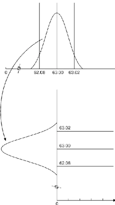
Assume that data produced by a process follows a normal distribution with a certain mean value and standard deviation. A control chart is another way to represent this distribution by rotating the distribution over 90 degrees. In this way, the mean becomes the centerline of the chart, while the upper and lower control limits of the chart correspond to the limits of a confidence interval. This is illustrated in Figure 1 below:
Essentially, a control chart is equivalent to testing the following two hypothesis: 𝐻0 : the process is in a state of statistical control 𝐻1 : the process is not in a state of statistical control
Whenever a point on the control chart falls within control limits, it is equivalent to not rejecting the null hypothesis and “accepting” that the process is in statistical control. On the other hand, if a point is located outside the control limits (i.e. “extreme points”), it is equivalent to rejecting the null hypothesis, thus implying the process is out-of-control. In other words, when there are extreme points, it may be a sign that an assignable cause has occurred, which has lead to a change (“shift”) in either the process mean value, or the process standard deviation, or a combination of both, thus leading to a state of lack of statistical control.
Figure 1: An illustration of the construction of a control chart. The distribution has been rotated 90 degrees. The centerline is the line corresponding to the mean value, the control limits are the lines corresponding to the limits of the 99,73% confidence intervals. Source: Winkel & Zhang (2007), pp. 15
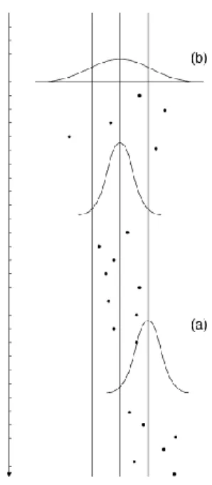
In Figure 2, three frames are present. The middle frame represents a state of statistical control. Frame (b) shows the pattern in case of an increase of the process standard deviation, while frame (a) demonstrates the behavior in case of an increase of the process mean.
It is important to mention that, beside extreme points, there are other possible indications for an out-of-control condition, such as a systematic or cyclic patterns in the plotted data. Montgomery (2013) describes the following ‘runs rules’ that can be used to find out whether the process being monitored is behaving abnormally:
Rule 1: One or more points outside of the control limits (extreme points) Rule 2: A run of eight consecutive points on one side of the center line Rule 3: Six consecutive points steadily increasing or decreasing Rule 4: Fourteen points in a row, alternating up and down
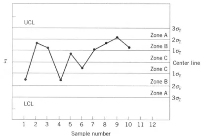
In theory, control charts are often constructed by placing the upper and lower control limit at a distance of three standard deviations from the center line. Consequently, control charts can be split into three zones (A, B, and C), on each side of the center line. This is illustrated in Figure 3.
Figure 2: The behavior of a chart in case of (a) an increase of the process mean, and (b) an increase of the process standard deviation.
These zones are used in the following run rules to detect an out-of-control condition:
Rule 5: Two of three consecutive points are more than 2 standard deviations from the center line
Rule 6: Four of five consecutive points are more than 1 standard deviation from the center line. In Figure 3, the last four points on the chart show a violation of rule 6.
Rule 7: Eight points in a row on both sides of the center line with none in zone C Rule 8: Fifteen points in a row in zone C (both above and below the center line)
Despite the availability of various established rules, it is remarkable that the majority of research papers that I consulted only make use of the standard rule of extreme points to analyze control charts. As a consequence, many of the charts that I discuss in my literature review (cf. Part 2) mainly focus on that rule.
3. Potential errors
Just as in hypothesis testing, a control chart may potentially make two types of error. A type I error is committed when the control chart signals out-of-control, even though in reality, the process is in control. Furthermore, a type II error happens when all observations fall within the control limits of the control chart, even though the process is out-of-control. This situation prevents the chart from signaling that the process is not in statistical control (Winkel & Zhang, 2007).
Such errors are not desirable, as they reduce the effectiveness of the chart. The degree to which a control chart makes such errors, determines the performance of the chart. Simply said, the fewer errors, the better the control chart.
4. Guidelines for chart selection
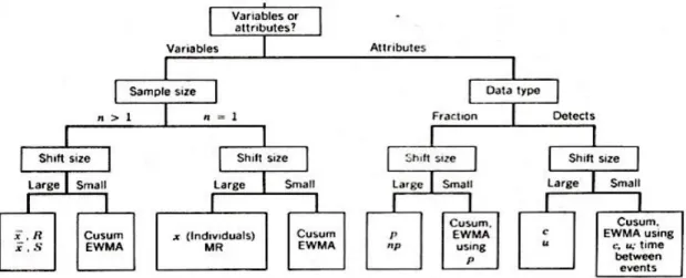
According to Chang and Wu (2011), the Shewhart charts, the CUSUM chart and the EWMA chart are the most frequently studied control charts in the literature. Montgomery (1991) summarized these popular charts in an overview (Figure 4) and proposed certain guidelines concerning which control chart to select for implementation.
The distinction between different charts is based on whether it is a chart for variables or attributes, the size of the sample, and / or the size of the shift that occurs in the process mean or standard deviation.
4.1. Variables versus attributes
Traditional control charts can be subdivided into two categories: charts based on variables and charts based on attributes. Attributes are quality characteristics that cannot be measured in a numerical manner. That is why they are classified as either “conforming” or “non-conforming” (Montgomery, 1991). On the other hand, variables can be expressed in terms of a numerical measurement, such as a dimension, weight, or volume (Montgomery, 1991).
4.2. Shift size
Control charts are also differentiated based on their ability to detect shifts in the process mean or standard deviation. Some charts are better in detecting large shifts, while other charts are more preferable in situations where a small shift occurs. For example, Winkel and Zhang (2007) mention that the CUSUM chart is more effective in detecting small shifts in the process mean, while it is not as effective as the X chart in detecting large changes in the process mean
4.3. Sample size
What is the importance of the sample size for control charts? In control charts, observations can be plotted as collections (samples) rather than plotting individual observations, as long as there is sufficient data to form samples. When designing a chart, it is tremendously important to think about the size of the samples that will be plotted. Why? Because larger samples will make it easier to detect small shifts in the process. If the process shift is relatively large, then smaller sample sizes will be used than those that would be employed if the shift of interest were relatively small (Montgomery, 1991).
5. Evaluation of a control chart
The performance of a control chart can be assessed by calculating its average run length (ARL), false alarm rate (FAR), or average time to signal (ATS). These measures make it possible to compare the performance of different charts in order to determine which chart outperforms the others.
5.1. ARL
Traditionally, average run length is the major criterion for measuring the performance of a control chart (Chang & Wu, 2011), if the sampling interval of data remains constant (Li, Zou, Ghong, &Wang, 2014). Researchers, such as Winkel and Zhang (2007), make a distinction between “in-control ARL” and “out-of-control ARL”.
The in-control ARL is the average number of points that must be plotted before a point indicates an out-of-control condition, when the process is in out-of-control (Montgomery, 1991). When a process is in out-of-control, it is always desirable to have a large ARL (Chang & Wu, 2009), to prevent the chart from incorrectly signaling that the process is out-of-control, and in this way, to decrease the false alarms. The in-control ARL can be calculated in the following way :
𝐴𝑅𝐿𝑖𝑛 𝑐𝑜𝑛𝑡𝑟𝑜𝑙 = 𝛼1 (2) in which 𝛼 is the probability of a type I error
Likewise, out-of-control ARL is the average number of points that must be plotted before a point indicates an out-of-control condition, when the process is out of control (Montgomery, 1991). A small ARL is preferable when an out-of-control condition has occurred in the chart (Chang & Wu, 2011), to detect a change or shift in the process as soon as possible. The out-of-control ARL can be calculated in the following way :
𝐴𝑅𝐿𝑜𝑢𝑡−𝑜𝑓−𝑐𝑜𝑛𝑡𝑟𝑜𝑙 = 1−𝛽1 (3)
in which 𝛽 is the probability of a type II error
An important remark that needs attention is the fact that the ARL is usually computed with the assumption that the process change is already present at the time that the chart is started (Lu & Reynolds, 1999). However, in practice, it may be that a process change occurs after the control chart has been running for some time. In that case, it is better to calculate the “steady-state average run length” (SSARL), which calculates the average number of samples / points that are plotted between the change to the signal, and not between the start of the chart to the signal (Lu & Reynolds, 1999).
The majority of researchers make use of the ARL as a performance metric. This is the reason why the control charts that I discuss in my literature review (cf. Part 2) exclusively focus on the ARL.
5.2. FAR
The false alarm rate is the probability that a control chart declares a process to be out-of-control, when in fact, it is in-control, i.e. a type I error (Krishnamoorthi & Krishnamoorthi, 2011). A control chart that has a smaller FAR than another chart, may be considered a better chart.
5.3. ATS
Li et al. (2014) define the average time to signal as the expected time from the start of the process to the time when the chart indicates an out-of-control signal. This performance indicator is widely used for control charts with variable sample intervals (VSI). When the process is in control, a chart with a larger ATS indicates a lower false alarm rate than other charts. When the process is out of control, a chart with a smaller ATS indicates a better detection ability of process shifts than other charts (Li et al., 2014).
Chapter 2: The Problem of Autocorrelation
Many researchers have demonstrated in their scientific findings that the presence of autocorrelation has an impact on the performance of control charts, including Montgomery and Mastrangelo (1991), Alwan and Roberts (1988), and Harris and Ross (1991). In this chapter, the phenomenon of autocorrelation in process data is explained. Some methods to detect, measure, and model the correlation are discussed. Finally, the impact of correlation on control charts is analyzed.
1. Autocorrelation: definition and sources
Gujarati and Porter (2009) define autocorrelation as “correlation between members of series of observations ordered in time or space”. In time series data, in which observations follow a natural ordering over time, successive observations are likely to exhibit intercorrelations, especially if the time interval between successive observations is short, for example an hour or a day, rather than a year (Gujarati & Porter, 2009).
Two particular examples of activities that may produce such autocorrelated data are (1) chemical processes, where measurements on process or product characteristics are often highly correlated, and (2) automated test and inspection procedures, where every quality characteristic is measured on every unit in time order of production (Montgomery, 2013).
One important source that leads to the formation of correlation is what researchers call “inertial elements” in a process (Harris & Ross, 1991). When inertia effects are present in a manufacturing process, the impact of a strange event that occurs during manufacturing, may only gradually and slowly exhibit itself instead of quickly and immediately. The example that was mentioned in the Introduction (the bottle filling process) is an illustration of inertia.
Montgomery (2013) states that all manufacturing processes are driven by such inertial elements, and combined with small sampling intervals, the observations will be correlated over time. In other words, correlation is not a phenomenon that occurs rarely. Therefore, it is relevant and useful to incorporate correlation into control chart methodology and analysis.
2. Detecting and measuring autocorrelation
There are two ways to find out whether the data contains a correlative structure. The first method of detection is the graphical way. The presence of autocorrelation can be easily derived in a graphical manner by plotting a process quality characteristic (𝑥𝑡) against time to observe how its value evolves over time. In case there is a
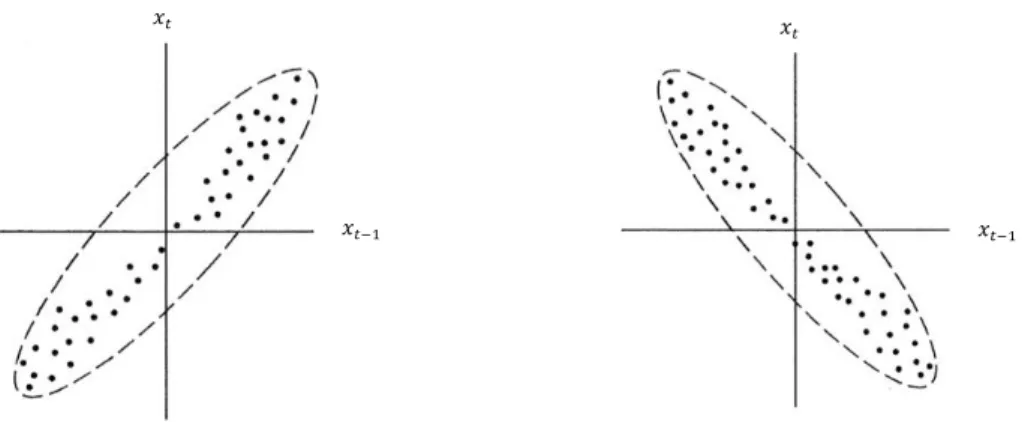
It is also possible to make use of a scatter plot in which an observation at time t (𝑥𝑡) is plotted against the observation one period earlier (𝑥𝑡−1) (i.e. lag 1). Figure 6 illustrates this method. If the points on the scatter plot
cluster around a line with a positive slope, it is a sign of positive autocorrelation. Likewise, if the points on the scatter plot cluster around a line with a negative slope, it is a sign of negative autocorrelation.
Next to the graphical method, a second way of detection consists of making use of a statistical test, such as the Durbin-Watson test. The Durbin-Watson statistic is often used in statistical regression analysis to test for autocorrelation in a data set. In that way it is possible to track down the presence of autocorrelation, and whether it is positive or negative.
Lu et al. (1999) and Montgomery (2013) mention an important aspect about detecting autocorrelation. When autocorrelation is observed, it is either (1) the result of an assignable cause, or (2) an inherent characteristic of the process. In the former case, the autocorrelation can be eliminated. But in the latter case, the autocorrelation can not be removed in the short run. Thus, when it is detected, it might be useful to first think whether there is a possibility to remove it.
Figure 5: Cyclic patterns indicate the presence of autocorrelation. Left graph: positive autocorrelation. Right graph: negative autocorrelation. Source: Gujarati & Porter (2009), pp. 419
Figure 6: Left scatter plot: positive autocorrelation. Right scatter plot: negative autocorrelation.
Source: Gujarati & Porter (2009), pp. 419
𝑥𝑡 𝑥𝑡
𝑥𝑡
𝑥𝑡−1
𝑥𝑡
Once autocorrelation is detected, it is interesting to measure the correlation in an analytical way. This provides information on the intensity of the correlation, whether the correlation is high or low. In case of time-series observations, the autocorrelation can be measured by the autocorrelation function (ACF), defined as
𝜌𝑘= 𝐶𝑜𝑣(𝑥𝑉𝑎𝑟(𝑥𝑡,𝑥𝑡−𝑘)
𝑡) =
𝛾𝑘
𝛾0 k = 0, 1, … (4)
in which 𝐶𝑜𝑣(𝑥𝑡, 𝑥𝑡−𝑘) is the covariance of observations that are k time periods apart, and 𝑉𝑎𝑟(𝑥𝑡) is the
variance of the observations. In practice, the values of 𝜌𝑘 are estimated with the sample autocorrelation
function, given by
𝑟𝑘 = ∑ ( 𝑥𝑡 − 𝑥̅ ) ( 𝑥𝑡−𝑘 − 𝑥̅ )
𝑛−𝑘 𝑡=1
∑𝑛𝑡=1 ( 𝑥𝑡 − 𝑥̅ )2 k = 0, 1, …, K (5)
with 𝑥̅ the mean of observations.
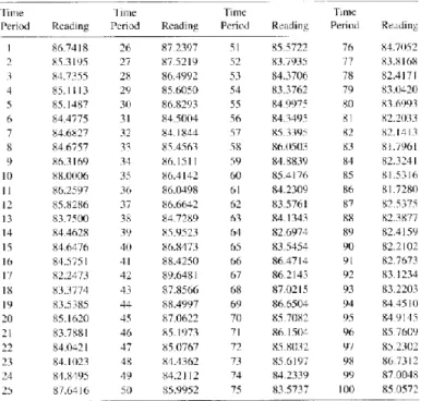
Detecting and measuring autocorrelation can also be done simultaneously. As an illustration, consider a chemical process of which the viscosity is being monitored (Montgomery, Jennings, Kulahci, 2008). The viscosity is measured at 100 different time points, which results in the data exhibited in Table 1.
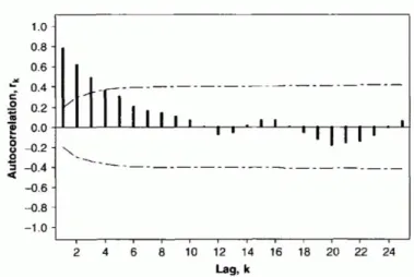
It is possible to visualize the sample autocorrelation function for this chemical viscosity data, to demonstrate how 𝑟𝑘 changes at different values of the lag k. This is illustrated in Figure 7.
Table 1: Viscosity readings from a chemical process
For each value of the lag, you can see whether there is positive / negative autocorrelation, and how large it is. The dashed lines represent 5% significance limits. If a sample autocorrelation 𝑟𝑘 exceeds the limit on the graph,
the corresponding autocorrelation value 𝜌𝑘 is likely non-zero. Figure 7 clearly reveals the presence of positive
autocorrelation in the chemical process data, equal to around 0.8 at lag = 1, 0.6 at lag = 2, and so on.
Such visualizations are often used to gain initial insights on the correlation in the data. For example, if the autocorrelation at lag 2 is equal to or around zero, then it would not be smart to model your data as a second-order autoregressive process (cf. the upcoming section 3.2. of Chapter 2). In practice, these visualizations can be created quite rapidly by using statistical software that generates such visualizations in a matter of seconds. In this way, you can easily find out whether your data is autocorrelated and measure how large the autocorrelation is.
3. Modeling autocorrelation
The correlative structure in process data can be directly represented with a model. One popular way to do this, is through Autoregressive Integrated Moving Average (ARIMA) models. Montgomery, Jennings and Kulahci (2008) discuss these time series models in great detail. The upcoming paragraphs are largely based on their work.
A time series is a time-oriented or chronological sequence of observations on a variable we are interested in. Thus, autocorrelated process data that gets plotted on a control chart can also be considered a time series. In this way, building a model around this time series delivers a “time series model”. The purpose of such modeling will be more clear as the reader gradually continues through the text.
One possible assumption in time series modeling is the assumption of stationarity. Some time series models are used to describe stationary process behavior, while others focus on nonstationary behavior. Stationarity implies a type of stability in the data. A time series is said to be strictly stationary if the probability distribution of observations 𝑥𝑡, 𝑥𝑡+1, ... , 𝑥𝑡+𝑁 is exactly the same as the probability distribution of observations 𝑥𝑡+𝑘, 𝑥𝑡+𝑘+1,
Figure 7: A sample autocorrelation function.
Source: Montgomery, Jennings & Kulahci (2008), pp. 32
… , 𝑥𝑡+𝑘+𝑁 in which k is a time interval. Another possibility is weak stationarity, which is valid if (1) the expected
value of the time series does not depend on time ( 𝐸(𝑥𝑡) = 𝜇 for all t ), if (2) the variance is a finite constant
value ( 𝑉𝑎𝑟(𝑥𝑡) = 𝜎2< ∞ for all t ), and if (3) the autocovariance function 𝐶𝑜𝑣(𝑥𝑡, 𝑥𝑡+𝑘) for any lag k is only a
function of k and not time. Whenever these conditions are not satisfied, the time series is said to be nonstationary, for example, when the time series exhibits a trend. Intuitively, stationary models assume that a process remains in equilibrium about a constant mean level (Vasilopoulos & Stamboulis, 1978).
In the next four sections, the ARIMA models are introduced. The first three models, i.e. MA(q) , AR(p) and ARMA(p,q), impose a stationarity condition, while the ARIMA(p,d,q) model does not impose such assumption.
3.1. MA(q)
As explained previously with equation (1), in case of no autocorrelation, observations can be represented as:
𝑦𝑡= 𝜇 + 𝜀𝑡 t = 1, 2, 3, … (6)
where 𝜀𝑡 is a random error that is normally and independently distributed with mean zero and standard deviation 𝜎𝜀. In the MA(q) model, a Moving Average process is used to represent correlated data. The dependency between observations is modeled through the random component 𝜀𝑡 in the following way :
𝑦𝑡= 𝜇 + 𝜀𝑡− 𝜃1𝜀𝑡−1 − ⋯ − 𝜃𝑞𝜀𝑡−𝑞 (7) where 𝑦𝑡 is the observation at time t, 𝜇 is the mean value, and where 𝜀𝑡 is white noise. White noise means that these random errors are uncorrelated, have mean zero and a constant variance.
Compared to equation (6), it is clear that now there are multiple disturbances 𝜀𝑡−𝑞 included. The parameter q is the order of the process, which gives the total number of past disturbances that is included in the model. Intuitively, this means that the observation at time t (𝑦𝑡) depends not only on its own disturbance 𝜀𝑡, but also on disturbances 𝜀𝑡−𝑞 of previous observations. 𝜃, the moving average parameter, is the weight that is given to a particular disturbance 𝜀𝑡−𝑞 , which tells us how much a particular disturbance contributes to the value of observation 𝑦𝑡.
The most basic moving average process is reached when the order q is equal to 1, referred to as the MA(1) process:
𝑦𝑡= 𝜇 + 𝜀𝑡− 𝜃1𝜀𝑡−1 (8) In this model, the correlation between 𝑦𝑡 and 𝑦𝑡−1 can be calculated with the following autocorrelation formula:
𝜌𝑦(1) = − 𝜃1
1+𝜃12 and 𝜌𝑦(𝑘) = 0 𝑓𝑜𝑟 𝑘 > 1 (9)
3.2. AR(p)
In an AutoRegressive process, an observation 𝑦𝑡 is directly dependent on its precedent observations 𝑦𝑡−1, 𝑦𝑡−2,
…, 𝑦𝑡−𝑝. The order p represents the number of past observations included in the model. The general p-th order
AR model has the following structure:
𝑦𝑡= 𝛿 + 𝜙1𝑦𝑡−1+ 𝜙2𝑦𝑡−2+ ⋯ + 𝜙𝑝𝑦𝑡−𝑝+ 𝜀𝑡 (10) in which 𝜙 is the autoregressive parameter that has a value |𝜙| < 1. 𝜀𝑡 is white noise, and 𝛿 = (1 − 𝜙)𝜇.
The most simple autoregressive process is the first-order autoregressive process (AR(1)) in which p is equal to 1: 𝑦𝑡= 𝛿 + 𝜙𝑦𝑡−1+ 𝜀𝑡 (11) If 𝜙 > 0, it is called positive autocorrelation, and 𝜙 < 0 implies negative autocorrelation. The larger | 𝜙 | is, the higher the correlation is, which means 𝑦𝑡−1 affects 𝑦𝑡 much more (Zhang, He, Zhang, & Wang, 2013).
In case of an AR(1) process, the autocorrelation function is given by : 𝜌𝑘 = 𝛾𝑘
𝛾0= 𝜙
𝑘 for k = 0, 1, 2, … (12)
Therefore, the correlation between 𝑦𝑡 and 𝑦𝑡−1 is 𝜙, the correlation between 𝑦𝑡 and 𝑦𝑡−2 is 𝜙2 and so on.
3.3. ARMA (p,q)
A third possible model can be obtained by taking the combinations of AutoRegressive and Moving Average terms, i.e. an ARMA(p,q) model. In general, this model is given as:
𝑦𝑡= 𝛿 + 𝜙1𝑦𝑡−1+ 𝜙2𝑦𝑡−2+ ⋯ + 𝜙𝑝𝑦𝑡−𝑝+ 𝜀𝑡 − 𝜃1𝜀𝑡−1 − 𝜃2𝜀𝑡−2 − ⋯ − 𝜃𝑞𝜀𝑡−𝑞
or 𝑦𝑡= 𝛿 + ∑𝑝𝑖=1𝜙𝑖𝑦𝑡−𝑖+ 𝜀𝑡 – ∑𝑞𝑖=1𝜃𝑖𝜀𝑡−𝑖 (13) This can also be formulated with a backshift operator ℬ, defined as ℬ𝑑𝑦
𝑡= 𝑦𝑡−𝑑:
Φ(ℬ)𝑦𝑡= 𝛿 + Θ(ℬ)𝜀𝑡 (14) with Φ(ℬ) = (1 − 𝜙1ℬ − 𝜙2ℬ2− ⋯ − 𝜙𝑝ℬ𝑝) and Θ(ℬ) = (1 −𝜃1ℬ − 𝜃2ℬ2− ⋯ −𝜃𝑞ℬ𝑞)
Montgomery (2013) provides a practical illustration in which the implementation of the ARMA model can be useful. He states that in chemical and process industries, first-order autoregressive process behavior is fairly common. On top of this autoregressive behavior, a random behavior might also be present. This random behavior can be due to the fact that the quality characteristic is measured in a laboratory that has a measurement error. Hence, the observed measurement 𝑦𝑡 then consists of both an autoregressive component plus random
variation. That is why an ARMA(p,q) can be used as the process model.
An example of such ARMA(p,q) model is the “first-order autoregressive, first-order moving average” ARMA(1,1) model, which is described as:
𝑦𝑡= 𝛿 + 𝜙1𝑦𝑡−1+ 𝜀𝑡 − 𝜃1𝜀𝑡−1 (15) where 𝑦𝑡 is the observation at time t, 𝛿 = (1 − 𝜙1)𝜇 , 𝜙1 the autoregressive parameter, 𝜃1 the moving-average parameter, 𝜇 the mean of the process, 𝜀𝑡 the random noise term at time t.
If, in equation (15) the autoregressive parameter is set to zero (𝜙1= 0), the resulting model then becomes a
MA(1) model. Similarly, if the moving-average parameter is set to zero (𝜃1= 0), the model becomes an AR(1) model. This is a clear illustration that the ARMA(p,q) model extends the moving average and autoregressive models by combining them into one.
3.4. ARIMA(p,d,q)
If the mean value of the process is not fixed, then the process is considered nonstationary. This type of behavior occurs in chemical processes if the process variable is “uncontrolled”, which means there are no actions taken to keep the variable close to a certain value (Montgomery, 2013). An example of such a nonstationary process is illustrated by Figure 8, which shows a linear trend in the data:
This process does not have a constant level (i.e. nonstationary), but it can be seen that different snapshots taken in time exhibit similar behavior (i.e. an increasing behavior). However, it is possible to get rid of the nonstationarity by taking the first differences. This first difference 𝑤𝑡 is simply the difference between
observation 𝑦𝑡 and observation 𝑦𝑡−1 of the previous time interval. In other words, the nonstationary time series
𝑦𝑡 is being converted into a stationary time series 𝑤𝑡 by applying a differencing technique. The first difference
𝑤𝑡 is denoted as:
𝑤𝑡 = 𝑦𝑡− 𝑦𝑡−1= (1 − ℬ)𝑦𝑡 (16)
or, for higher-order differences: 𝑤𝑡 = (1 − ℬ)𝑑𝑦𝑡
Furthermore, such a time series 𝑦𝑡 is called an AutoRegressive Integrated Moving Average process of orders p,
d, and q (i.e. ARIMA(p,d,q)) if its dth difference produces a stationary ARMA(p,q) process.
Generally, an ARIMA(p,d,q) can be written as: Φ(ℬ)(1 − ℬ)𝑑𝑦
𝑡= 𝛿 + Θ(ℬ)𝜀𝑡 (17) The ARIMA(p,d,q) model is an extension of the previously explained ARMA(p,q) model. If no difference were to be taken in the modelling (i.e. d = 0), the resulting ARIMA(p,0,q) model would be equal to the ARMA(p,q) model denoted in equation (14).
The simplest nonstationary model is the ARIMA(0,1,0), also called “the random walk process”, written as: (1 − ℬ)𝑦𝑡= 𝛿 + 𝜀𝑡 (18) Figure 8: A plot of a nonstationary process
Source: Montgomery, Jennings & Kulahci (2008), pp. 233
Another example is the ARIMA(0,1,1) process, which is given by:
(1 − ℬ)𝑦𝑡= 𝛿 + (1 −𝜃ℬ)𝜀𝑡 (19)
which is also known as the integrated moving average IMA(1,1) process.
Overall, the ARIMA model is in fact a more general model formulation that encapsulates all previous models. For example, the ARIMA(1,0,0) is also the AR(1) model. And, the ARIMA(0,0,1) is the MA(1) model.
4. Effects of autocorrelation on the performance of a control chart
In this fourth and last section of Chapter 2, the impact of autocorrelation on control charts is described to inform the reader about the performance deterioration that is caused by the presence of autocorrelation.According to Lu and Reynolds (1999), autocorrelation typically has two negative effects. First, it can lead to a decrease of the in-control ARL, which implies a higher false alarm rate than in the case of independent observations. Secondly, it can lead to an increase of the out-of-control ARL, which implies an increase in the time required to detect changes in the process.
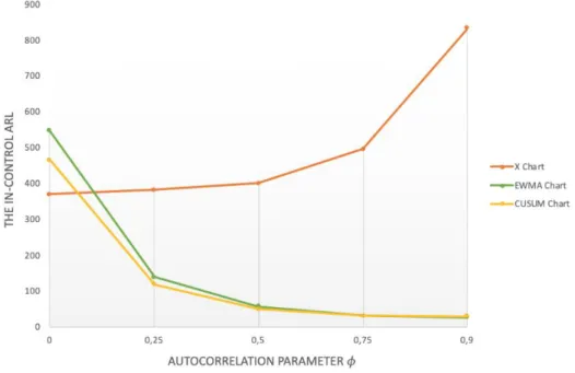
Both of these effects are mentioned in Zhang (2000) his work as well. His research includes a simulation study for first-order autoregressive processes (AR(1)) with the autoregressive parameter of the process 𝜙 equal to the values 0, 0.25, 0.50, 0.75 and 0.90. This autocorrelated process data was used to construct an X-chart, CUSUM chart and EWMA chart. Then, their performance was assessed by measuring their in-control ARL and out-of-control ARL. These ARLs are obtained from simulations for shifts of the process mean of size 0, 0.5, 1, 2, and 3, expressed in terms of the process standard deviation. The in-control ARL corresponds to the situation where the shift is equal to 0. And the out-of-control ARL is for the scenarios where the mean shift is larger than 0. In total, 25 different scenarios were possible, and the ARL of the charts changed depending on the parameter values of a scenario (for example, the scenario where 𝜙 = 0.25 with a mean shift of 1 standard deviation, resulted in an out-of-control ARL of 46.61 for the X-chart). Table 2 summarizes the average run lengths in tabular form:
A correlation coefficient (𝜙) equal to zero means that the sequence of process data becomes an independent and identically distributed (i.i.d.) sequence (Zhang, 2000). By comparing the scenario in which the correlation coefficient has a value zero (i.e. there is no autocorrelation), with the other scenarios in which the coefficient is assigned a value different from zero, the impact of autocorrelation can be derived from Table 2. The data from Table 2 is visualized on Figure 9 and 10 to make it easier to understand. From these visualizations, two effects can be observed, corresponding to the findings of Lu & Reynolds (1999) (cf. supra):
1) Impact on the in-control ARL (Figure 9):
Figure 9 depicts the in-control ARL for all three control charts, which is the ARL when there is no change in the process mean (“Shift” = 0). For the CUSUM chart and EWMA chart, the in-control ARL decreases when the autocorrelation coefficient increases. In other words, a higher degree of correlation (higher 𝜙) leads to more false alarms in a CUSUM chart and EWMA chart, which is undesirable. However, this is only the case for the CUSUM and EWMA charts, not the X chart.
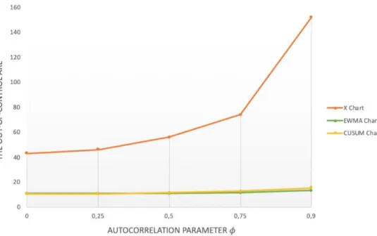
2) Impact on the out-of-control ARL (Figure 10):
Figure 10 shows the out-of-control ARLs, which is the ARL when there is a change in the process (“Shift” > 0). It is immediately clear that, for the X chart, the out-of-control ARL increases when the autocorrelation coefficient increases. For example, in case of Shift = 1 and increasing 𝜙, the ARL changes in the following way:
Figure 9: In-control ARLs of the X chart, EWMA chart, CUSUM chart, for different values of 𝜙. Source: Visualisation by Aytaç Kurtulus, based on
In other words, a higher degree of correlation (higher 𝜙) leads to a deterioration of the detection capability of an X-chart because more time will be needed to detect a process change. But, this is not the case for the EWMA and CUSUM charts.
These previous examples clearly demonstrate that autocorrelation can disturb different control charts in a different way. Due to these disturbances, wrong conclusions will be made about the state of statistical control of the process being monitored. This problem gave the incentive for researchers to start developing new methods and charts to use in case of autocorrelation. Part 2 of this dissertation discusses these methods in great detail.
Figure 10: Out-of-control ARLs of the X-chart, EWMA chart, CUSUM chart, for different values of 𝜙. Source: Visualisation by Aytaç Kurtulus, based on
Part 2: Control Charts for autocorrelation: a literature
review
Introduction
It is a given fact that control chart literature is a quite extensive research topic. In order to provide some insight into the general structure of the available literature, it is possible to categorize the research in the following way:
Firstly, a distinction can be made between univariate control charts and multivariate control charts. In the case of multivariate control charts, multiple quality characteristics are monitored at the same time. For example, a mechanical bearing that has an inner diameter 𝑥1 and outer diameter 𝑥2 that, together, determine the usefulness
of the part (Montgomery, 2013).
The second domain concerns the parameter being monitored. Some researchers focus on charts that monitor the process mean, while others focus on monitoring the process variability. Furthermore, the simultaneous monitoring of mean and variance is also a research area.
Thirdly, when autocorrelated data is represented with a model, a distinction can be made between linear models and non-linear models. The ARIMA process is a popular example of linear modeling. On the other hand, research that uses non-linear modeling is also available, such as Schipper and Schmid (2001), who focused on Generalized Autoregressive Conditional Heteroskedasticity (GARCH) processes.
Finally, there is a difference between monitoring variables versus monitoring attributes. When a process produces continuous data, then we make use of variables. On the other hand, attribute data is discrete, such as the number of defects in a manufacturing process.
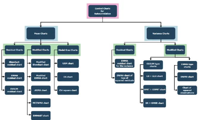
To narrow down the subject of the dissertation, I opt to focus on univariate control charts for autocorrelation, that monitor the mean or the variance, and that make use of ARIMA modeling if necessary. All control charts for autocorrelation that will be discussed are summarized in Figure 11. It is important to mention that all of these charts focus on monitoring a variable, not an attribute. Because variable control charts for autocorrelation are the most widely discussed in the literature, while research on attribute control charts for autocorrelation is less popular.
In Chapter 3 of Part 2, Mean Charts are explained. This is followed by all the Variance Charts in Chapter 4. In general, there are three main approaches to deal with autocorrelation. One approach makes use of conventional control charts with adjustments to the method of calculating the control limits in order to account for the autocorrelation (Lu & Reynolds, 1999). Lu and Reynolds (1999) argue that this approach can be applied especially when the level of autocorrelation is not extremely high. These adjusted charts are referred to as Modified Charts.
Another approach consists of fitting an appropriate time series model, such as the ARIMA models discussed in Part 1, to the process data. This model is then used to make forecasts (predictions) of each observation using the previous observations (Lu & Reynolds, 1999). By taking the difference between observation 𝑥𝑡 and its fitted value
𝑥̂𝑡, the residuals or forecast errors 𝑒𝑡 are calculated: 𝑒𝑡= 𝑥𝑡− 𝑥̂𝑡. Then, control charts can be applied to these
residuals, resulting in so called Residual Charts. This is possible given the fact that these residuals will be approximately normally and independently distributed with mean zero and constant variance (Montgomery, 2013). Montgomery and Mastrangelo (1995) and other researchers argue that a system change, such as an assignable cause, will increase the absolute magnitude of the residuals. Indeed, when there is a change in the process mean or variance, the time series model that was identified will no longer be a correct representation of the data (i.e. a “misspecification”). This misspecification will be transferred to the residuals (Montgomery & Mastrangelo, 1991). Thus, applying control charts to residuals makes it possible to detect a process change.
Finally, a less popular approach are the model-free charts. These are control charts for autocorrelation that do not apply any modeling techniques to the data. They can be considered as a separate category of charts where
no residuals are used or modifications to existing charts are made. However, model-free charts are mainly applied for monitoring the mean. I believe there is no significant research that investigates model-free charts for monitoring the variance.
In the upcoming chapters of Part 2, all control charts included in Figure 11 are explained in detail. After Part 2, some of these control charts will be implemented during a simulation study in Part 3, to gain (new) insights about the charts. In this way, a theoretical explanation is provided first, followed by the execution of a practical implementation.
Chapter 3: Control Charts for Monitoring the Mean
This chapter is subdivided into three sections: residual charts, modified charts, and model-free charts.
1. Residual charts
Alwan and Roberts (1988) proposed to make use of the autoregressive integrated moving average (ARIMA) models originally developed by Box and Jenkins (1976), to model the correlated data. This modeling decomposes the correlated data into an “actual”, “fitted” and “residual” part: Actual = Fitted + Residual. Consequently, the approach leads to two charts to be used jointly:
1) Common-Cause Chart (CCC): this chart is a plot of the fitted (predicted) values obtained through the ARIMA models. Wardell, Moskowitz and Plante (1994) comment that this chart is not a real control chart as it contains no control limits. Instead, “it serves as a snapshot of the current level of the process and is useful for dynamic process control”, which means it can be used to know whether or not certain corrective actions are needed. As Alwan and Roberts state, “the chart is useful to better understand how the process is working”.
2) Special-Cause Chart (SCC): a traditional control chart (Shewhart, CUSUM, or EWMA) that is applied to the residuals. The aim is to detect any special causes using the traditional ways. In the literature, the SCC chart is often referred to as the “Residual Chart”.
Jiang, Tsui and Woodall (2000) mention that the basic idea behind this SCC chart is to apply filtering techniques (i.e. the ARIMA modeling) to “whiten” an autocorrelated process, and then monitoring the residuals by traditional control charts. This “whitening” means that you obtain data that will be serially independent, i.e. the residuals.
There are three popular SCC charts mentioned in the literature: the Shewhart residual chart, the EWMA residual chart, and the CUSUM residual chart. Their implementation is similar to their traditional methods, but instead of the original observations, residuals are used. All three control charts are explained in this chapter. The methodology is illustrated for autocorrelated data that is representable as an AR(1) process. However, this is not the only possibility. For example, Lu and Reynolds (1999) illustrated that an EWMA chart can also be applied to the residuals of an ARMA(1,1) process.
The control limits mentioned in the next three paragraphs to construct the Shewhart residual chart, EWMA residual chart and CUSUM residual chart are provided by Osei-Aning et al. (2017).
1.1. The Shewhart residual chart
Assume an AR(1) process represented as (Runger & Willemain, 1995):
with 𝑥𝑡 the observed time series at time t, 𝜀𝑡 the white noise term, μ the mean, 𝜙1 the autocorrelation
coefficient. Next, to allow the possibility that a shift in the process mean occurs, a time-varying mean is included in the equation:
𝑥𝑡= 𝜇𝑡 + 𝜙1(𝑥𝑡−1− 𝜇𝑡−1) + 𝜀𝑡 (21)
By estimating the parameters of the equation, one can obtain the predicted value 𝑥̂𝑡 of 𝑥𝑡, with 𝑥̂𝑡=
𝜇(1 − 𝜙1) + 𝜙1𝑥𝑡−1. The difference between the real observation 𝑥𝑡 and its predicted value 𝑥̂𝑡 yields the
residuals 𝑒𝑡: 𝑒𝑡= 𝑥𝑡− 𝑥̂𝑡. These residuals will approximate the white noise 𝜀𝑡 and have negligible
autocorrelation.
In the Shewhart residual chart, the residuals 𝑒𝑡 are used as the plotting statistic. The control limits are
constructed as follows:
𝑈𝐶𝐿 = 𝜇 + 𝐿𝜎𝑒
𝐶𝐿 = 𝜇 𝐿𝐶𝐿 = 𝜇 − 𝐿𝜎𝑒
In which 𝜇 is the in-control mean of the residuals, equal to zero. 𝜎𝑒 is the standard deviation of the residuals. 𝐿
is a control chart multiplier, used to adjust the in-control ARL of the chart.
The standard deviation 𝜎𝑒 can be estimated by calculating moving ranges of the residuals (Montgomery, 2013).
Then, the average of the moving ranges has to be divided by a constant, as in the following formula: 𝜎𝑒=
𝑀𝑅 ̅̅̅̅̅ 𝑑2
With 𝑀𝑅̅̅̅̅̅ the average of the moving ranges, and 𝑑2 is a given constant. The specific value of 𝑑2 depends on the
number of observations that is taken in the moving range. For example, if the moving range consists of two residuals, 𝑑2 is equal to 1.128. The values for 𝑑2 and other similar factors can be retrieved from the table in
Appendix 1.
1.2. The EWMA residual chart
For the EWMA residual chart, the EWMA statistic that will be plotted is given by:
𝑍𝑡= 𝜆𝑒𝑡+ (1 − 𝜆)𝑍𝑡−1 (26)
with 𝜆 the smoothing parameter 0 ≤ 𝜆 ≤ 1. In order to detect small shifts, small values for 𝜆 are preferred and vice versa. The initial value 𝑍0 can be taken equal to the in-control mean of the residuals, which is zero. Just as in the case of the traditional EWMA chart, the control limits of the EWMA residual chart are initially not constant. Instead, the control limits reach a constant value after some time. These steady-state control limits can be calculated as follows: 𝑈𝐶𝐿 = 𝜇 + 𝐿𝜎𝑒√( 𝜆 2 − 𝜆) 𝐶𝐿 = 𝜇 𝐿𝐶𝐿 = 𝜇 − 𝐿𝜎𝑒√( 𝜆 2 − 𝜆) (25) (22) (23) (24) (27) (28) (29)
with 𝐿 the control constant in the chart.
1.3. The CUSUM residual chart
An important characteristic of the CUSUM chart is the possibility to make use of a ‘decision interval value’, instead of control limits, to test whether there is an out-of-control condition.
For the CUSUM residual chart, the upper and lower CUSUM statistics are defined as:
𝐶𝑡+= max (0, 𝑒𝑡− 𝜇 − 𝐾 + 𝐶𝑡−1+ ) (30)
𝐶𝑡−= max (0, 𝜇 − 𝑒
𝑡− 𝐾 + 𝐶𝑡−1+ ) (31)
with the reference value 𝐾 = 𝑘𝜎𝑒 and decision interval value 𝐻 = ℎ𝜎𝑒. A widely used value for k is 0.5 and an
acceptable value for H is five times 𝜎𝑒 (Osei-Aning et al., 2017). The CUSUM residual chart will signal when a
CUSUM statistic exceeds 𝐻 , or:
𝐶𝑡+> 𝐻 𝑜𝑟 𝐶𝑡−> 𝐻 (32)
1.4. Remarks on the residual chart’s performance
Wardell et al. (1994) provide several reasons why the approach of Alwan and Roberts are appealing, including: (a) It takes advantage of the fact that the process is correlated to make forecasts of future quality
(b) the special-cause chart is based on the assumption that the residuals are random, and hence any of the traditional tools for SPC can be used
(c) the special-cause control chart can be used to detect any assignable cause, including changes in the structure of the time series
(d) the model can be applied to any type of time series model and it is not limited to AR(1) or MA(1) time series
(e) the method is more effective in detecting shifts in the process mean than more traditional control charts when the underlying process is ARMA(1,1).
Other remarks concerning this approach are provided by Alwan and Roberts themselves. They admit that making use of time series models is not an easy task, as there is certain statistical knowledge necessary to implement them. However, they also add that most practical applications can be approximated with the simplest ARIMA models (such as the first-order integrated moving average process ARIMA(0,1,1)), ensuring that the implementation is less demanding than it first appears. On top of that, they argue that statistical computer tools (such as Minitab) can be used to apply the ARIMA modeling in an automated way.
2. Modified charts
Despite the popularity of residual charts, many researchers have proven that a residual chart is not the “perfect” solution to the problem of autocorrelation as it does not offer the desired performance in all circumstances.