INDICATORS AND MODELLING OF
LAND USE, LAND MANAGEMENT
AND ECOSYSTEM SERVICES
Methodological documentation
Katalin Petz, Catharina J.E. Schulp, Emma H. van der Zanden, Clara Veerkamp, Mart-Jan Schelhaas, Gert-Jan Nabuurs, Geerten Hengeveld
Indicators and modelling of land use, land management and ecosystem services. Methodological documentation.
© PBL Netherlands Environmental Assessment Agency The Hague, 2016
PBL publication number: 2386 Contact
Arjen.vanHinsberg@pbl.nl Authors
Katalin Petz (PBL), Catharina J.E. Schulp (VU University Amsterdam), Emma H. van der Zanden (VU University Amsterdam), Clara Veerkamp (PBL), Mart-Jan Schelhaas, Gert-Jan Nabuurs and Geerten Hengeveld (all Wageningen Environmental Research)
Acknowledgements
The authors would like to thank Arjen van Hinsberg, Anne Gerdien Prins and Henk van Zeijts (PBL) for the project coordination, and Sandy van Tol (PBL) and Jan Clement (Wageningen Environmental Research) for the assistance in the GIS work.
Graphics
PBL Beeldredactie
Production coordination PBL Publishers
This publication can be downloaded from: www.pbl.nl/en. Parts of this publication may be reproduced, providing the source is stated, in the form: Petz et al. (2016), Indicators and modelling of land use, land management and ecosystem services. Methodological
documentation. PBL Netherlands Environmental Assessment Agency, The Hague. PBL Netherlands Environmental Assessment Agency is the national institute for strategic policy analysis in the fields of the environment, nature and spatial planning. We contribute to improving the quality of political and administrative decision-making by conducting outlook studies, analyses and evaluations in which an integrated approach is considered paramount. Policy relevance is the prime concern in all our studies. We conduct solicited and unsolicited research that is always independent and scientifically sound.
Contents
1
INTRODUCTION
5
2
LAND-USE MODELLING
7
2.1 CLUE land-use-change simulations 7
2.2 Technical details of land-use-change modelling 8
2.2.1 Land-use classification 8
2.2.2 Location-specific preference additions 13
2.2.3 Land-use conversions 17
2.2.4 Conversion elasticities 18
2.2.5 Neighbourhood settings 19
3
LAND MANAGEMENT DRIVERS
21
3.1 Agricultural intensity 21
3.2 Forest management 22
3.3 Green landscape elements 24
4
ECOSYSTEM SERVICES MODELLING
26
4.1 Indicators for ecosystem services 26
4.1.1 Overview 26
4.1.2 Technical issues 27
4.2 Wild food provision 27
4.2.1 Methodology 27 4.2.2 Discussion 34 4.3 Carbon sequestration 35 4.3.1 Methodology 35 4.3.2 Discussion 38 4.4 Flood regulation 39 4.4.1 Methodology 39 4.4.2 Discussion 43 4.5 Erosion prevention 44 4.5.1 Methodology 44 4.5.2 Discussion 48 4.6 Pollination 50 4.6.1 Methodology 50 4.6.2 Discussion 55 4.7 Pest control 57
4.8 Recreation 62 4.8.1 Methodology 62 4.8.2 Discussion 65
5
POTENTIAL IMPROVEMENTS
68
REFERENCES
69
APPENDIX
77
Appendix 1 77 Appendix 2 79 Appendix 3 84 Appendix 4 91 Appendix 5 101 Appendix 6 105 Appendix 7 1081 Introduction
Background
Ecosystems provide numerous benefits to people by supplying food, fresh water, fertile soils, timber and recreation opportunities, among others. Generally, ecosystem services can be classified into provisioning (e.g. food, drinking water, wood fuel) regulating-maintenance services (e.g. climate regulation, erosion control, pollination) and cultural services (e.g. aesthetic information, recreation, educational value). Changes in land use and its intensity are main drivers of ecosystem services change. Land conversion and land-use intensification have led to the degradation of ecosystems, biodiversity and ecosystem services across the globe (MA, 2003, 2005; Petz, 2014).
Ecosystem services have been assessed increasingly from national to European and international levels, over the last decades. The first international policy assessment with a comprehensive overview of the consequences of ecosystem change for human well-being was the Millennium Ecosystem Assessment (MA, 2003, 2005). This was later followed by the study on The Economics of Ecosystems and Biodiversity (TEEB, 2008, 2010), which gave an insight into the economic significance of ecosystems. Currently, a new standardised
classification system, the Common International Classification of Ecosystem Services (CICES), is being developed by the European Environment Agency. The CICES classification builds on the existing classifications (MA, TEEB) and is aimed at a better understanding of how ecosystem services relate to particular economic activities or products and facilitate ecosystem accounts (Haines-Young and Potschin, 2011, 2013). Mapping and assessing biodiversity and ecosystem services1 is at the core of the EU Biodiversity Strategy to 2020
(European Commission, 2011).
Ecosystems and the services they provide are being degraded across Europe. The EU has set targets for 2020 to halt the loss of biodiversity and improve the state of ecosystem services. The EU Biodiversity Strategy formulates this as follows: ’Halting the loss of biodiversity and the degradation of ecosystem services in the EU by 2020, and restoring them in so far as feasible, while stepping up the EU contribution to averting global biodiversity loss’ (European Commission, 2011).
Aim of the report
This report provides background information on modelling of land use, land management and ecosystem services (Figure 1.1). This work was carried out in close collaboration with the VU University Amsterdam and Wageningen Environmental Research. The main drivers of
ecosystem services change were considered to be land cover/land use (Chapter 2), agricultural intensity, forest management and the presence of green landscape elements (Chapter 3). These drivers feed into the ecosystem services models (Chapter 4). These models are suitable for conducting large-scale simulations and for answering policy-relevant questions, such as ‘How could changes in land use influence ecosystem services, such as soil erosion prevention and recreation capacity of the landscape in Europe?’.
The models described here, were, among others, used in the Nature Outlook project of PBL Netherlands Environmental Assessment Agency (Van Zeijts et al., forthcoming) to assess the
effects of a Trend scenario. The results of the model runs are reported in detail in
Perspectives on the future of nature: impacts and combinations (Prins et al., forthcoming). Figure 1.1.
2 Land-use modelling
2.1 CLUE land-use-change simulations
Land-use changes are modelled with a CLUE-scanner (Pérez-Soba et al., 2010; Verburg et al., 2012; Verburg et al., 2011), a multi-scale, multi-model framework that combines various sector models, a land-use-allocation model and indicator models, connecting analyses on global and European scales to local environmental impacts (Figure 2.1).
The Dyna-CLUE model, implemented in the CLUE-scanner, simulates competition between land uses, combined with spatial allocation rules that define location suitability for land-use types, conversions between land-use types, impact of spatial policies, and neighbourhood characteristics (Verburg et al., 2010). Regrowth of natural vegetation was simulated as a function of the local growing conditions, and pressures from human population density, grazing and management (Verburg et al., 2010). The model uses a 1-year time step, 1 km2 spatial resolution and
distinguishes 17 land-use types, based on a spatially and thematically aggregated version of the CLC2000 land-cover map (EEA, 2000; Overmars et al., 2014; Schulp et al., 2016). Figure 2.1 shows the procedure for land-use-change allocation.
There are four ‘boxes’ of information needed to model land-use changes: • Spatial policies and restrictions on land-use change (e.g. Natura 2000);
• Land-use requirements in terms of area demand for agriculture, urban development or nature;
• Location characteristics and maps that define the suitable location for each land-use type based on empirical analysis. For example, the European soil map can be translated into functional properties, such as soil fertility and water retention capacity. In addition to the soil map, there is a set of 100 factors that range from accessibility to bio-physical
properties; the factors can be dynamic in time (e.g. in case of population which is based on scaling down EUROSTAT NUTS level projections). A full list of the factors considered can be found in Verburg et al. (2006);
• A set of rules on possible conversions between use types (conversion elasticity, land-use transition sequences).
For each time step, land-use demand is allocated on the basis of location characteristics, land-use-specific conversion settings and spatial policies and restrictions. The allocation is done as follows:
• The suitability for each land-use type throughout Europe is calculated;
• A preliminary land-use allocation is made by allocating the land-use type with the highest suitability to each 1 km2 grid cell;
• The preliminary allocation is then compared with the demand;
• If the preliminary allocation does not match the demand, the competitive advantage of the land-use types is adapted and a new preliminary allocation is made;
• The first four steps are repeated until the demand has been fulfilled;
• The allocation takes into account spatial policies and restrictions by excluding designated areas from land-use changes. Rules for possible conversions between land-use types are accounted for by excluding certain land-use conversions or by increasing the suitability of land-use types relative to each other, thus making the conversion from one type of land use into another more likely. This procedure is elaborated in Section 2.3.
2.2 Technical details of land-use-change modelling
2.2.1 Land-use classification
The CLUE land-use classification system used in the CLUE-scanner was also used for ecosystem services modelling. Table 2.1 describes the 16 CLUE land-use classes used in the Nature Outlook. The CLUE classes can be easily translated into the CORINE classes (Table A1 in Appendix 1).
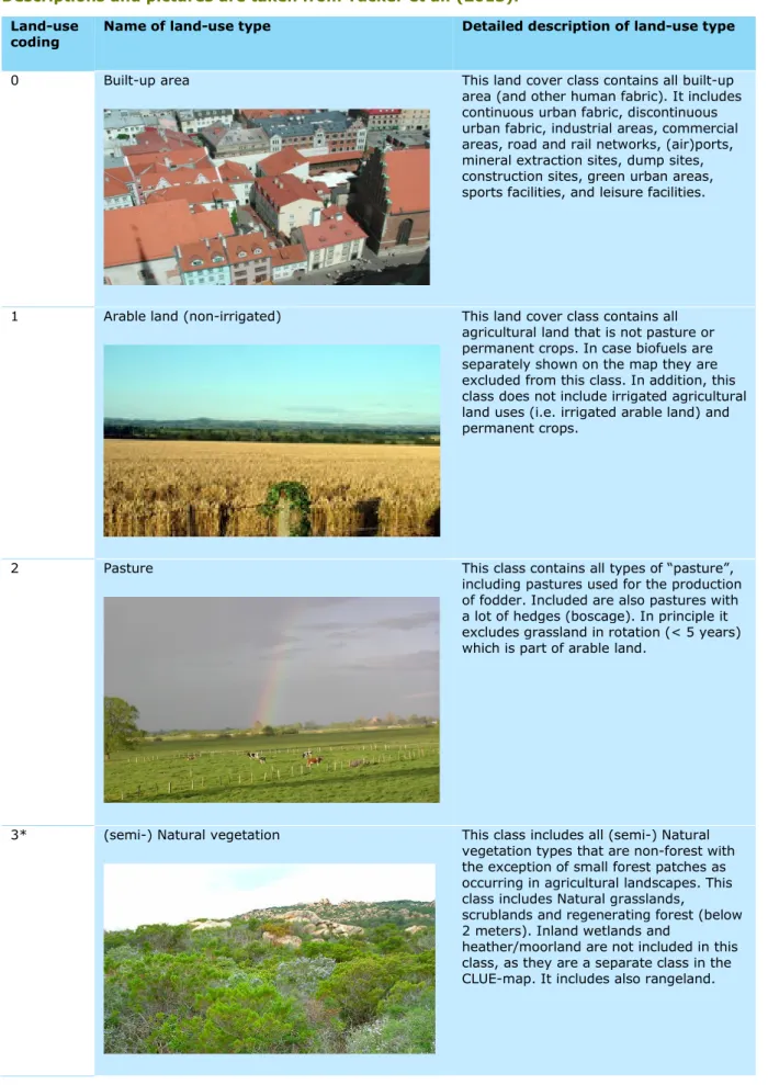
Table 2.1. Detailed description of CLUE land-use types used in the Nature Outlook. Descriptions and pictures are taken from Tucker et al. (2013).
Land-use
coding Name of land-use type Detailed description of land-use type
0 Built-up area This land cover class contains all built-up area (and other human fabric). It includes continuous urban fabric, discontinuous urban fabric, industrial areas, commercial areas, road and rail networks, (air)ports, mineral extraction sites, dump sites, construction sites, green urban areas, sports facilities, and leisure facilities.
1 Arable land (non-irrigated) This land cover class contains all agricultural land that is not pasture or permanent crops. In case biofuels are separately shown on the map they are excluded from this class. In addition, this class does not include irrigated agricultural land uses (i.e. irrigated arable land) and permanent crops.
2 Pasture This class contains all types of “pasture”, including pastures used for the production of fodder. Included are also pastures with a lot of hedges (boscage). In principle it excludes grassland in rotation (< 5 years) which is part of arable land.
3* (semi-) Natural vegetation This class includes all (semi-) Natural vegetation types that are non-forest with the exception of small forest patches as occurring in agricultural landscapes. This class includes Natural grasslands,
scrublands and regenerating forest (below 2 meters). Inland wetlands and
heather/moorland are not included in this class, as they are a separate class in the CLUE-map. It includes also rangeland.
4** Inland wetlands This class covers all inland wetlands and peat bogs. Only standing waters are included in this land cover class. Flowing rivers and other water courses are included in a separate class.
5** Glaciers and snow This class covers all glaciers and permanent snow.
6 Irrigated arable land This class contains all irrigated agriculture/arable land. It includes rice fields, but not greenhouses, and spray/rotary sprinklers.
7* Recently abandoned arable land This class contains recently abandoned arable land that is no longer used in a crop rotation. It includes very extensive farmland not reported in agricultural statistics. It consists of herbaceous vegetation, grasses and shrubs below 30 cm. This class naturally transgresses into the class “(semi-) Natural vegetation”. Most of this land cover type is still classified as arable land or permanent crops in the input data for the CLUE-map. Therefore, this class will only evolve during the simulations.
8 Permanent crops This class contains all land cover classes that are associated with permanent crops. It includes all kinds of agro-forestry classes, such as dehesas and montanas.
10 Forest The forest class contains production forest, protected forest, and forest not currently harvested for other reasons. It does not include other types of natural vegetation, nor does it contain agro-forestry land cover types.
11** Sparsely vegetated areas This class contains all land cover types that are extremely sparsely vegetated. It includes bare rock and, badlands, etc.
12** Beaches, dunes and sands This class includes land cover types such as beaches, dunes and sands in general.
13** Salines This class contains salt pans, but excludes salt marshes.
14** Water and coastal flats All water surfaces and coastal flats
15** Heathland and moorlands Vegetation with low and closed cover, dominated by bushes, shrub and herbaceous plants (heather, briars, broom, gorse, laburnum). Most often succession into forest vegetation is constraint by climate or soil conditions.
16* Recently abandoned pasture land This class contains recently abandoned pasture land. It includes very extensive pasture land not reported in agricultural statistics. It consists of herbaceous vegetation, grasses and shrubs below 30 cm. This land cover class contains vegetation that is no longer production grassland but cannot yet be considered Natural grassland. It may be under very extensive grazing regime not being respected in agricultural statistics. This may include horse keeping. This class Naturally transgresses into the land cover class “(semi-) Natural vegetation”. Most of this land cover type is still classified as pasture land in the land use map of the year 2000. Therefore, this class will only evolve during the simulations.
* These classes are considered to be an intermediate stage in the natural succession from recently abandoned farmland to (semi-) natural vegetation. Under certain conditions, succession will be so slow that the vegetation
** These land-use types are assumed to be constant during simulations with CLUE. These areas are assumed to be unsuitable for agriculture or urban expansion. This assumption is based on the adverse environmental conditions at these locations. Natural succession is also assumed to be hampered by adverse environmental conditions.
2.2.2 Location-specific preference additions
Spatial policies can change the suitability for a certain land use at a certain location. For example, farming can continue on areas less suitable for arable production based on soil and climatic due to Less-Favoured Area (LFA) subsidy. Such an effect of a policy is modelled by increasing the
suitability of a location for a land-use type in areas to which the policy is targeted (Figure 2.1, top left box). Default values for the changes in suitability due to the location-specific preference additions representing the spatial policies, have been defined. . Table 2.2 lists the default settings for spatial zonings and Table 2.3 describes the maps. Table 2.4 describes the weight assigned to the location-specific preference addition maps in the modelling of land-use change.
Table 2.2. Default location-specific preference additions used in modelling land-use changes. ‘X’ indicates that a spatial zoning is included in the location-specific preference additions.
Spatial zoning Default settings
Natura 2000 areas X
LFA areas cropped in the year 2000 X National protected areas
Areas with a high provision of regulating and cultural ecosystem services
Areas with a high erosion risk X Semi-natural areas in the year 2000
Areas that are cropped in the year 2000* X
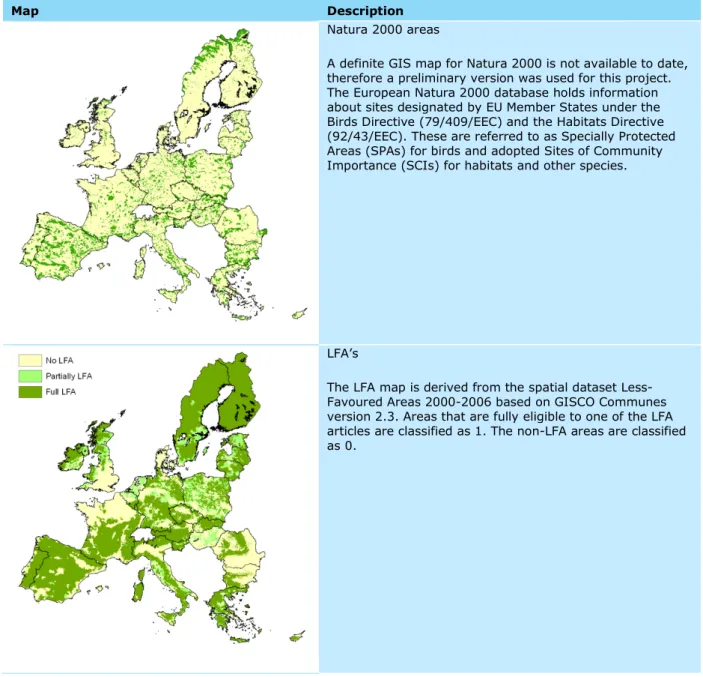
Table 2.3. Maps of location-specific preference additions. Descriptions and pictures are taken from Tucker et al. (2013).
Map Description
Natura 2000 areas
A definite GIS map for Natura 2000 is not available to date, therefore a preliminary version was used for this project. The European Natura 2000 database holds information about sites designated by EU Member States under the Birds Directive (79/409/EEC) and the Habitats Directive (92/43/EEC). These are referred to as Specially Protected Areas (SPAs) for birds and adopted Sites of Community Importance (SCIs) for habitats and other species.
LFA’s
The LFA map is derived from the spatial dataset Less-Favoured Areas 2000-2006 based on GISCO Communes version 2.3. Areas that are fully eligible to one of the LFA articles are classified as 1. The non-LFA areas are classified as 0.
National protected areas
Map of WDPA areas up to IUCN category IV (IUCN and WDPA, 2013).
Ecosystem services and biodiversity areas
This map identifies areas with a low, moderate or high potential for ecosystem services supply or biodiversity. For this, a map of the bundle of regulating services was used. The ES bundle map is the sum of the normalised services. A map of bird species richness in 2000 was normalised and added. The map was reclassified to distinguish the hotspots (areas with values in the upper quartile of the values distribution) and cold spots (areas with values in the lower quartile of the values distribution).
Erosion sensitive areas
Delineation of areas with a high potential for soil erosion. Derived from a potential soil erosion map that was computed as the product of slope, soil erodibility and rain erosivity. A threshold was identified by making an overlay with current arable land, whereby it was aimed that approximately 8% of current arable land would be eligible for receiving subsidies to prevent soil erosion.
(Semi)natural areas
Delineation of natural and semi-natural vegetation in the year 2000.
Forest areas
Delineation of forested areas in the year 2000.
Cropped areas
Table 2.4. Description and weight of location-specific preference addition maps for the default settings.
Land-use code and name Default settings
0 Urban
1 Rain fed arable 0.2 in currently cropped LFA areas 2 Pasture 0.2 in currently cropped LFA areas 3 Semi-natural
4 Irrigated arable
5 Recently abandoned arable
6 Permanent crops 0.2 in currently cropped LFA areas 7 Forest
8 Recently abandoned pasture 9 Static land use types
2.2.3 Land-use conversions
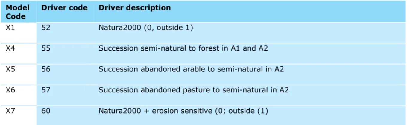
‘Allow drivers’ are maps that define locations where certain land-use conversions are or are not allowed (e.g. protected areas), or where there are temporal constraints on certain conversions (e.g. succession time). These allow driver maps contain the spatially explicit settings as used in the conversion matrices. Table 2.5 gives a description of these drivers. The model codes indicated by ‘X..’ refer to the specific allow driver maps in the CLUE-scanner framework and the driver codes are used in the conversion matrices. Drivers specifying temporal constraints indicate the maximum or minimum years after which a conversion can or should take place.
Table 2.5. Description of spatial restrictions maps.
Model
Code Driver code Driver description
X1 52 Natura2000 (0, outside 1)
X4 55 Succession semi-natural to forest in A1 and A2 X5 56 Succession abandoned arable to semi-natural in A2 X6 57 Succession abandoned pasture to semi-natural in A2 X7 60 Natura2000 + erosion sensitive (0; outside (1)
Table 2.6 presents the used conversion matrix for the Trend scenario. This table indicate which land-use conversions are allowed. Values of 1 indicate that the conversion is allowed, values of 0 indicate that the conversion is not allowed. Other numbers refer to the spatial restrictions maps listed in Table 2.5. For example, a conversion from semi-natural to arable land is allowed outside Natura 2000 sites. Inside Natura 2000 sites such change is not allowed (code 52).
Table 2.6. Conversion matrix for the Trend scenario. Values of 1 indicate that the conversion is allowed, values of 0 indicate that the conversion is not allowed. Other numbers refer to the spatial restrictions maps listed in Table 2.5.
Conversion to B ui lt-up A ra bl e Pa stur e S em i-na tur al Ir ri ga te d ar ab le la nd A ba nd one d ar ab le Pe rm ane nt cr op s Fo rest A ba nd one d pa stu re O the r C u rr ent la nd us e Built-up 1 0 0 0 0 0 0 0 0 0 Arable 1 1 1 0 0 1 1 0 0 0 Pasture 1 1 1 0 0 0 1 0 1 0 Semi-natural 1 52 52 1 0 0 52 55 0 0 Irrigated arable land 0 0 0 0 1 0 0 0 0 0 Abandoned arable 1 52 52 56 0 1 52 0 0 0 Permanent crops 1 1 1 0 0 1 1 0 0 0 Forest 1 52 52 0 0 0 52 1 0 0 Abandoned pasture 1 52 52 57 0 0 52 0 1 0 Other 0 0 0 0 0 0 0 0 0 1
2.2.4 Conversion elasticities
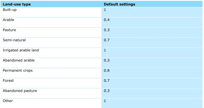
The conversion elasticities (Table 2.7) determine how easily a certain land use can be converted into another and are therefore a proxy for the conversion costs (0 = very easy to convert and 1 is very difficult to convert). These values are based on expert knowledge and calibration of earlier applications of this modelling framework (Verburg and Overmars, 2009).
Table 2.7. Conversion elasticities. Values of 1 indicate the conversion is difficult, values of 0 indicate the conversion is easy.
Land-use type Default settings
Built-up 1
Arable 0.4
Pasture 0.3
Semi-natural 0.7
Irrigated arable land 1
Abandoned arable 0.3 Permanent crops 0.8 Forest 0.7 Abandoned pasture 0.3 Other 1
2.2.5 Neighbourhood settings
The neighbourhood settings determine how the land-use allocation depends on the land use in the surrounding areas, and this is used to determine the fragmentation patterns. For each land-use type, a fraction of the suitability that is defined by neighbourhood settings is specified (Table 2.8). This varies between zero (no impact of land use in surrounding areas) to 1 (allocation fully based on land use in surrounding areas). Second, the size of the surrounding area is specified for each land-use type (Table 2.9). The values are chosen on the basis of the scenario specifications and calibrated on the basis of previous model applications (Verburg and Overmars, 2009).
Table 2.8. The fraction of the location suitability that is determined by land use in the surrounding areas. Value of ‘0’ indicates there is no such influence, and ‘1’ indicates that the land use in the surrounding area fully determines the allocated land use.
Land-use type Default settings
Built-up 0.3
Arable 0
Pasture 0
Semi-natural 0
Irrigated arable land 0
Abandoned arable 0
Permanent crops 0
Forest 0
Abandoned pasture 0
Other 0
Table 2.9. Cells considered for calculating neighbourhood effects. The ‘0’ value indicates the cell for which these effects were calculated. Values >0 represent the cells used for calculating neighbourhood effects, including their awarded weight, ranging from 0.001 to 1.
Land-use type Default settings
Built-up 11111 11111 11011 11111 111112
3 Land management
drivers
This chapter describes the characteristics of the land management drivers used in the ecosystem, modelling (Table 3.1). Maps for the drivers serving as input in the ecosystem service models were created for the Trend scenario (year 2000 and 2050).
Table 1.1. Land management drivers considered.
Land management
drivers Unit Source
Agricultural intensity 5 classes CAPRI-CLUE modelling (Temme and Verburg, 2011) Forest management 5 classes Forest Management Approaches (Duncker et al., 2012;
Hengeveld et al., 2012) implemented in EFISCEN model (Schelhaas et al., 2007)
Green elements Number of intersects Tieskens et al. (submitted)
3.1 Agricultural intensity
We built on the methodology of Temme and Verburg (2011), who proposed to use a combination of European level databases to construct land-use intensity maps with separate methodologies for arable land and grassland.
Nitrogen application was used as an indicator for the intensity of arable land management. Data at the highest spatial resolution available are on NUTS2/3 level. For each administrative unit, nitrogen input levels are reported per crop type collected within the Farm Structure Survey (FSS) and the Land Use/Cover Area frame statistical Survey (LUCAS) (Gallego and Delincé, 2010). LUCAS provides point-based observations of crop types from 2006, for about 150,000 sample points across agricultural areas in the EU. Each point of the LUCAS data set was assigned the crop-specific nitrogen application rate reported in the FSS data set for the corresponding administrative unit, assuming that variation in nitrogen application within an administrative unit may be approximated by the cropping pattern. Nitrogen application rates were then classified into three classes: low (<50 kg/ha); medium (50–150 kg/ha) and high (>150kg/ha) (Overmars et al., 2014) (Table 3.2). Based on these observations of nitrogen application rates, the probability of occurrence of each intensity class at a specific location was explained by a set of environmental and socio-economic locational factors using multinomial regression. Locational factors included are topographic conditions, soil and climate conditions, population densities and accessibility. A list of all factors included is provided by Temme and Verburg (2011).
For grassland a different approach was taken as for arable land, also as described by Temme and Verburg (2011). For the LUCAS observations of grassland, the nitrogen input was estimated based on the local stocking densities with cattle. Stocking densities were derived from the livestock maps of Neumann et al. (2009). We assumed a uniform quantity of 100 kg N/ha per cow per year and reclassified the observations into two classes: intensive grassland with > 50 kg N/ha and extensive grassland with < 50 kg N/ha (Table 3.2). Similar to the procedure for arable land, country-specific logistic regression models are estimated and used within the administrative units for scaling down
The estimated regression models were used to predict the intensity class on each location classified as arable land or pasture. This was done based on the areas required for each intensity class following CAPRI simulations for specific years. The regression models were estimated for all countries. For the countries without LUCAS data (Czech Republic, Slovakia, Hungary, Romania and Bulgaria), we used regressions estimated from neighbouring countries with comparable agricultural practices. For Croatia and Switzerland, intensity classes were derived from (Monfreda et al., 2008). Maps of fertiliser and manure input were added together, smoothed and expanded to the missing border cells by a 75 km circle focal mean, extracted for cropland and grassland in the year 2000 and reclassified following the three classes: low (<50 kg/ha); medium (50–150 kg/ha) and high (>150 kg/ha). Figure 3.1 shows the land-use intensity for 2000.
Table 3.2. Explanation of the agricultural intensity map.
Intensity
class Explanation Ellenberg N range Intensity class Explanation Ellenberg N range
1 Extensive Arable land, <50
kg N/ha 3–6 4 Extensive Pasture, <50 kg N/ha 3–7 2 Moderately
intensive Arable land, 50–150 kg N/ha 5–8 5 Intensive Pasture, 50–150 kg N/ha 6–9 3 Intensive Arable land, >150
kg N/ha 7–9
Figure 3.1.
3.2 Forest management
provide projections under alternative scenarios. It was originally developed for Sweden (Sallnäs, 1990) and later applied to the whole of Europe to explore the future of forests, including growth rate, climate impacts and carbon budgets (Nabuurs et al., 2006; Schelhaas et al., 2007). The model was also used, among others, in the European Forest Sector Outlook Study (United Nations et al., 2011) and the VOLANTE EU project for exploring the future of the European forestry sector and modelling forest ecosystem services.
The EFISCEN model works at the aggregated level of provinces to national level, depending on the forest area and data availability. The initial state of the forest and the current growth are derived from detailed measurements, usually done by the respective National Forest Inventory (NFI). For use in the model, the data are aggregated to regions, tree species, site classes and/or ownership (‘forest types’). Data needed are area, average growing stock and average growth per age class for each of these combinations, for each country under study. The state of the forest is described by a distribution of area over age and volume classes; the development over time is determined by natural processes (e.g. growth and mortality) and influenced by management regimes (i.e. thinning, final felling, choice of tree species in regeneration) and changes in forest area.
Management can be optimised for different targets, such as biodiversity conservation and wood energy maximisation. The initialisation data used in Nature Outlook are the same as in VOLANTE. More details on the EFISCEN initialisation data can be found in the VOLANTE project documentation (Lotze-Campen et al., 2013). The Trend scenario in the Nature Outlook is based on the A2 scenario of the VOLANTE project. A description of the scenario implementation and the model framework can be found in the VOLANTE project documentation (Lotze-Campen et al., 2012).
To run the EFISCEN model, information about wood demand, afforestation/deforestation, changes in growth level as a consequence of climate change and (changes in) forest management are needed. Five forest management approaches (FMA) are distinguished (Duncker et al., 2012) (Table 3.3), explicitly mapped over Europe (Hengeveld et al. 2012). Suitability of a certain location for each FMA is based on 1) dominant tree species, 2) biogeographic region, 3) slope, 4) proximity to smaller cities, 5) proximity to larger cities, 6) percentage of forest cover, 7) stand area, and 8) Natura2000 coverage. The factors are weighted based on expert knowledge. The resulting map indicates the suitability of a location for a particular FMA. Separate maps for the individual FMAs are merged into a single map by attributing the FMA with the highest suitability to each location. Comparison of this map with forest inventory data from the Netherlands and Umbria showed that the FMA map consistently slightly underestimated the intensity of the management regime (Hengeveld et al., 2012). This was confirmed in a comparison with country-level statistics. The map is documented in more detail in Hengeveld et al. (2012). The forest map is static potential forest management map, i.e. only available for the year 2000 (Figure 3.2). Actual forest area was clipped for the year 2000 and 2050. Except for the area of forest, no changes were assumed for 2050.
Based on an overlay of the species map (Brus et al., 2012) and the potential FMA map (Hengeveld et al., 2012), we identified for each species how much area is managed according to a certain FMA, for the base land-use map of 2000. Each of these FMAs was run separately in the EFISCEN model. FMA3 is managed with limited interventions to balance economic and ecological objectives. FMA4 and FMA5 have intensive management with shortened rotations of 10 and 20 years, respectively. FMA2 has a prolonged rotation of 20 years to mimic natural processes, and FMA1 is unmanaged (Duncker et al., 2012; Hengeveld et al., 2012). The matching of the species represented in EFISCEN and those in the map by Brus et al. (2012) is similar to that in Schelhaas et al. (2015). First, FMA5 was deducted from the national wood demand, then FMA4 was deducted from the remaining demand, and so on.
all FMA runs were aggregated to the country level and subsequently scaled down to a 1 km2
gridded species map (Brus et al., 2012).
Table 3.3. Forest Management types.
FMA Explanation
1 Unmanaged nature reserves 2 Close-to-nature forestry 3 Mixed objective forestry 4 Intensive even-aged 5 Short-rotation forestry
Figure 3.2.
3.3 Green landscape elements
Green linear landscape elements (GLs) are hedgerows and tree lines across the landscape. The map of the presence of green lines from Tieskens et al. (submitted) was used for the year 2000 (Figure 3.3). Regarding the extrapolation for 2050, our assumption was that at places where agricultural field size is small (i.e. smaller than 10 ha) and agriculture becomes more intensive, green elements disappear by 2050. For agricultural field size, the map from Kuemmerle et al. (2013) was used. The map of Tieskens et al. (submitted) excludes Croatia. Therefore, for Croatia we assumed no GLs.
There is another map of green lines by Van der Zanden et al. (2013). The main difference between the two maps is that Van der Zanden et al. (2013) used the LUCAS 2009 database with different
specific regression, whereas Tieskens et al. (submitted) used the LUCAS 2012 database and simple kriging. The map of Van der Zanden et al. (2013) excludes Croatia, Romania, Bulgaria and
Switzerland, whereas as the map of Tieskens et al. (submitted) excludes only Croatia. We tested that using another GL map has little effect on the ecosystem services results.
4 Ecosystem services
modelling
This chapter describes the ecosystem services models used in the Nature Outlook and model settings for the Trend scenario. Furthermore, examples for output maps are presented and uncertainties are discussed. Because of their generic character, the ecosystem services models could be applied also beyond the Nature Outlook.
4.1 Indicators for ecosystem services
4.1.1 Overview
Seven GIS-based ecosystem services models are described that can assess scenario effects for wild food provision, carbon sequestration, flood regulation, erosion prevention, pollination, pest control and recreation. Six of the ecosystem services models (wild food provision, carbon sequestration, flood regulation, erosion prevention, pollination and recreation) were adopted from the VU
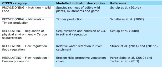
University Amsterdam. Most models are developed within the CONNECT project. Most models have been applied for European scale policy support before (Schulp et al., 2016; Tucker et al., 2013). The pest control model was developed by PBL building on earlier works. The models can be classified as ‘intermediate complexity’ models, which are suitable for large-scale simulations but are closely based on scaled up results of more process-based models (Schulp et al., 2014b). Timber production was simulated with the EFISCEN model (Schelhaas et al., 2007) run by Wageningen Environmental Research. A full model documentation is provided by Schelhaas et al. (2007) and this model is not further described here. Table 4.1 provides an overview of the studied ecosystem services following the CICES classification (Maes et al., 2015) and their modelled indicator.
Table 4.1. Overview of the included ecosystem services.
CICES category Modelled indicator description Reference
PROVISIONING – Nutrition – Wild
Food Species richness of edible wild plants, mushrooms and game Schulp et al. (2014a) PROVISIONING – Materials –
Timber production Timber production Schelhaas et al. (2007) REGULATING – Regulation of
physical environment – Carbon sequestration
Sequestration and emission of CO2
in soil and vegetation Schulp et al. (2008) REGULATING – Flow regulation –
flood regulation Relative water retention in river catchment Stürck et al. (2014) and (2015b) REGULATING – Flow regulation –
REGULATING – Regulation of
biotic environment – Pollination Percentage of cropland that can be accessed by pollinators from natural habitat
Serna-Chavez et al. (2014)
REGULATING – Regulation of
biotic environment – Pest control Pest predation rate (in %) This report (Petz et al. 2016) CULTURAL – Intellectual and
Experiential–Recreation Capacity of the landscape to support recreation Van Berkel and Verburg (2011)
4.1.2 Technical issues
The coverage of the study is EU 29 (EU 28 + Switzerland). For wild food and recreation, the modelling was done without Switzerland and Croatia (EU-27). Land-use simulations and indicator simulations were done based on a WGS1972 Albers Conical Equal Area projection. A 1 km spatial resolution was used. All models, except those on flood regulation, are available as ArcInfo AML scripts and ArcInfo Model Builder version. The flood regulation model combines MatLAB calculations and ArcGIS Model Builder components. The pest control model is available only in ArcInfo Model Builder. For the carbon sequestration, erosion prevention and pollination r scripts are available.
4.2 Wild food provision
4.2.1 Methodology
Table 4.2. The main characteristics of the wild food availability model.
Indicator name Wild food availability
Short description Species richness of a set of vascular plant, mushroom, and game species that are collected and consumed throughout Europe
Units Number of species Spatial resolution 1 km2
Temporal resolution Start and end year of simulation Output maps Game species richness;
Mushroom species richness; Vascular plant species richness; Total wild food species richness; Wild food sufficiency / variety index Main reference Schulp et al. (2014a)
Table 4.2 gives an overview of the main characteristics to simulate wild food supply in Europe (Schulp et al, 2014a). Figure 4.1 gives a schematic overview of the model and the input and output data are described in Table 4.3. The AML model script is presented in Appendix 2. Because of the data availability, simulation is only applied to the EU-27 (without Switzerland and Croatia). The model from Schulp et al. (2014a) has also a component to simulate wild food demand in Europe.
Table 4.3. Input and output parameters of the wild food availability model.
Name Unit Source Description
INPUT
Land cover CLUE classes (16) CLUE modelling CLUE land-cover map 1x1 km
Agricultural intensity 5 classes CLUE modelling Agricultural intensity measured by N input Forest management 5 classes EFISCEN modelling Forest management map Species distribution Presence/absence (≥50
km resolution) IUCN (IUCN, 2012), Birdlife International (2012) and the Atlas Flora Europaea (Lahti and Lampinen, 1999)
Broad-scale distribution maps of wild food species
Probability of occurrence
(≥50 km resolution) Guisan and Thuiller (2005) and Thuiller et al. (2009)
Consensus map of probability of occurrence of species for which no distribution maps were available. Calculated with Biomod2 platform. Habitat suitability values Yes (1) / No (0) Delbaere et al. (2009) Habitat suitability values
based on CORINE land cover
Yes (1) / No (0) Delbaere et al. (2009), Ellenberg and Lauschner (Ellenberg and
Lauschner, 2010)
Habitat suitability values based on agricultural land-use intensity Yes (1) / No (0) Delbaere et al. (2009),
ETI Bioinformatics (2013), IUCN (2012), Bundesambt für Naturschutz (2001)
Habitat suitability values based on forest
management
Infrastructure Yes (1) / No (0) PBL (2011) Major roads and railroads
OUTPUT
Game/mushroom/plant
availability Species number Richness of wild plant, mushroom or game species (#)
Wild food availability Species number Total wild species richness (#) Wild food sufficiency /
variety index Categorical variable (see description) Indication if wild food species are absent, available in limited richness, or available in abundant richness
Wild food availability was measured as the species richness of a set of vascular plant, mushroom, and game species that are collected and consumed in a grid cell. In the wild food availability model (2014a), an indicator for species richness of main wild food species is used that was based on an extensive literature review about wild food consumption (Eggers et al., 2009; Louette et al., 2010; Overmars et al., 2014). The indicator was calculated from data on species occurrence and their sensitivity to environmental pressures (Delbaere et al., 2009), namely land-use and management changes. The impact of land-use and management change is expected to be an important driver for wild food species in the coming decades and is therefore chosen as the environmental pressure of interest.
In the literature review of Schulp et al. (2014a), wild food species collected and consumed in the EU were identified. This included 97 game species, 152 mushroom species and 592 vascular plant species. While the collection and consumption of most of these species is restricted to a specific EU region, a subset of species is commonly collected and consumed throughout Europe. This included 38 game species, 27 mushroom species and 89 vascular plant species. This subset is used to map the spatial variability of wild food availability. A few species were not included because of lack of spatial data. The final species selection is given in Table 4.4, Table 4.5 and Table 4.6.
Table 4.4. Mushroom species included in wild food supply model.
Latin name Code Latin name Code
Agaricus arvensis MR1 Lactarius sanguifluus MR14 Agaricus campestris MR2 Leccinum scabrum MR15 Agaricus silvaticus MR3 Lepista nuda MR16 Armillaria mellea MR4 Macrolepiota procera MR17 Boletus edulis MR5 Morchella esculenta MR18 Cantharellus cibarius MR6 Pleurotus ostreatus MR19 Clitocybe odora MR7 Russula cyanoxantha MR20 Craterellus cornucopioides MR8 Suillus grevillei MR21 Fistulina hepatica MR9 Suillus luteus MR22 Hydnum repandum MR10 Suillus variegatus MR23 Hygrophorus eburneus MR11 Tricholoma terreum MR24 Laccaria amethystine MR12 Tuber aestivum MR25 Lactarius deliciosus MR13 Xerocomus chrysenteron MR26
Table 4.5. Vascular plant species included in the wild food supply model.
Latin name Code Latin name Code Latin name Code
Achillea millefolium VP1 Fragaria vesca VP31 Ribes rubrum VP61 Allium ampeloprasum VP2 Hippophae rhamnoides VP32 Ribes uva-crispa VP62 Allium schoenoprasum VP3 Humulus lupulus VP33 Rosa canina VP63
Allium ursinum VP4 Juniperus communis VP34 Rosa pouzinii VP64 Amelanchier ovalis VP5 Lathyrus tuberosus VP35 Rosa tomentosa VP65 Argentina anserina VP6 Laurus nobilis VP36 Rosmarinus officinalis VP66 Arum italicum VP7 Malus sylvestris VP37 Rubus caesius VP67 Asparagus acutifolius VP8 Malva sylvestris VP38 Rubus chamaemorus VP68 Berberis vulgaris VP9 Matricaria chamomilla VP39 Rubus fruticosus VP69 Bunium bulbocastanum VP10 Mentha aquatica VP40 Rubus idaeus VP70 Calamintha nepeta VP11 Mentha arvensis VP41 Rubus loganobaccus VP71 Capparis spinosa VP12 Mentha longifolia VP42 Rubus ulmifolius VP72 Capsella bursa-pastoris VP13 Mentha pulegium VP43 Rumex acetosa VP73 Carum carvi VP14 Mentha spicata VP44 Rumex acetosella VP74 Castanea sativa VP15 Mentha suaveolens VP45 Salvia officinalis VP75 Celtis australis VP16 Myrtus communis VP46 Sambucus nigra VP76 Chenopodium album VP17 Nasturtium officinale VP47 Scolymus hispanicus VP77 Chenopodium
bonus-henricus VP18 Origanum heracleoticum VP48 Silene vulgaris VP78 Cichorium intybus VP19 Origanum vulgare VP49 Sonchus oleraceus VP79 Cirsium arvense VP20 Oxalis acetosella VP50 Sorbus aucuparia VP80 Cornus mas VP21 Papaver rhoeas VP51 Taraxacum officinale VP81 Corylus avellana VP22 Petroselinum crispum VP52 Thymus serpyllum VP82 Crataegus monogyna VP23 Plantago lanceolata VP53 Tussilago farfara VP83 Cynara cardunculus VP24 Portulaca oleracea VP54 Urtica dioica VP84 Daucus carota VP25 Prunus avium VP55 Vaccinium myrtillus VP85 Diplotaxis tenuifolia VP26 Prunus spinosa VP56 Vaccinium oxycoccos VP86 Elymus repens VP27 Prunus virginiana VP57 Vaccinium uliginosum VP87 Eruca sativa VP28 Ranunculus ficaria VP58 Vaccinium vitis-idaea VP88 Ficus carica VP29 Ribes alpinum VP59 Viola odorata VP89 Foeniculum vulgare VP30 Ribes nigrum VP60
Table 4.6. Game species included in the wild food supply model. Effects of habitat fragmentation are considered for the species presented in bold italic.
Latin name Code Latin name Code Latin name Code
Alces alces GA1 Coturnix coturnix GA12 Sus scrofa GA23 Alectoris rufa GA2 Dama dama GA13 Tetrao tetrix GA24 Anas clypeata GA3 Gallinago gallinago GA14 Turdus merula GA25 Anas crecca GA4 Lepus europaeus GA15 Anser anser GA26 Anas penelope GA5 Lepus timidus GA16 Anser fabalis GA27 Anas platyrhynchos GA6 Oryctolagus
cuniculus GA17 Lagopus lagopus GA28
Anas querquedula GA7 Perdix perdix GA18 Phasisnus colchicus GA29
Capra pyrenaica GA8 Rangifer tarandus GA19 Streptopelia
decaocto GA30 Capreolus capreolus GA9 Rupicapra
rupicapra GA20 Tetrao urogallus GA31
Cervus elaphus GA10 Scolopax
rusticola GA21
Columba palumbus GA11 Streptopelia turtur GA22
The calculation rules are as follows (also see Figure 4.1):
1. For each species, coarse-scale presence/absence maps are created. These originate from IUCN (IUCN, 2012), Birdlife International (2012) and the Atlas Flora Europaea (Lahti and Lampinen, 1999). Where no coarse distribution patterns were available, the probability of occurrence was estimated using species distribution models (Guisan and Thuiller, 2005) within the biomod2 platform (Thuiller et al., 2009). Biomod2 uses an ensemble modelling approach that relates species’ occurrences to selected influential environmental variables and enables examination of species–environment relations throughout a wide range of modelling techniques (Thuiller et al., 2009). The output is a consensus probability map ranging from 0 to 1. The probability of occurrence was here modelled based on occurrence data from the Global Biodiversity Information Facility (GBIF) (Yesson et al., 2007). Isothermality, temperature seasonality, temperature annual range, mean temperature of coldest quarter and annual precipitation from WorldClim (Hijmans et al., 2005) were used as dependent variables. Occurrence probability maps were then converted into binary presence/absence maps using a threshold maximising the predictive accuracy of the models.
2. These coarse-scale presence/absence maps are scaled down by using habitat suitability maps based on land cover and intensity. These maps are created as follows:
a) For each species, a 1km resolution habitat map was made by reclassifying the land-use map from the CLUE-scanner. The habitat map indicates if the land-land-use type is suitable for the species (1) or not (0). This judgement of suitability was done based on habitat suitability values of each land-use type for each species (Delbaere et al., 2009). These habitat suitability values were based on CORINE land cover. For all land-use types, with the exception of built-up areas, we considered the maximum of the CORINE suitability levels given by Delbaere et al. (2009) representative for
the CLUE land-use class. For built-up areas, we used the median instead, given the underrepresentation of green elements suitable for wild flora and fauna.
b) For each species, a map of the agricultural land-use intensity (Potter et al., 2010; Temme and Verburg, 2011) was reclassified into a habitat suitability map indicating if the land-use intensity is suitable for the species (1) or not (0). Suitability ratings showing if a game or mushroom species occur in an agricultural intensity class were based on Delbaere et al. (2009), ETI Bioinformatics (2013) and IUCN (2012). Descriptions of species’ response to agricultural intensity were translated into a suitability by expert judgement. For plant species, the suitability for occurrence of agricultural intensity classes were based on the Ellenberg ranges (Ellenberg and Lauschner, 2010) and Delbaere et al. (2009). Ellenberg values were translated into suitability under the assumption that if the Ellenberg N range under which a species can occur overlaps with the Ellenberg range of the agricultural intensity class (Table 3.2), then the species can occur in that intensity class (Overmars et al., 2014). c) The impact of forest management was included based on the FMA map. The FMA
map was reclassified into a habitat suitability map indicating if the forest
management type is suitable for the species (1) or not (0). Information of species’ response to forest intensity from Delbaere et al. (Delbaere et al., 2009), ETI Bioinformatics (ETI Bioinformatics, 2013) and IUCN (IUCN, 2012) was translated into a suitability based on expert judgement. For plants, we based the suitability on the hemerobic range as given by the Bundesambt für Naturschutz (2001).
Hemeroby gives an indication for the human impact on the environment. We assumed that (1) species restricted to Hemeroby class A occur in unmanaged forests; (2) species with class O occur in close-to-nature forestry systems (3) species with Hemeroby classes M and B occur in mixed objective forestry, and species that can occur in Hemeroby classes C, P, and T can occur in intensive even-aged and short-rotation systems. Every habitat suitability is given in Appendix 4. 3. The habitat suitability maps based on land cover and intensity and the 50 * 50 km resolution
presence (1) / absence (0) map are multiplied, resulting in a 1 km resolution map of potential presence / absence of each species.
4. A few species are sensitive to fragmentation of their habitat (Delbaere et al., 2009). For these species a map of the habitat patch size (obtained from the previous step) intersected with the roads and railroads was created. Following Alkemade et al. (2009), suitability of patches with a size <500 km2 was set to zero.
5. Species richness maps are calculated by adding together the maps of the previous steps. 6. The wild food variety / sufficiency index indicates if wild food species are absent, available in
limited richness, or available in abundant richness. To calculate the indicator, firstly, the plant species richness and mushroom species richness maps were added together. Secondly, the plants and mushroom species richness as well as the game species richness were classified into the classes absent (0), species richness lower than median (1), and species richness equal to or higher than median (2) (Table 4.7). Static values from the simulation base year were used to ensure comparability of the index over years. Threshold values are 18 species for plants and mushrooms, and 7 species for game. Thirdly, the index is calculated as: WFSIndex = (10 * game classified map) + plants&mushrooms classified map. The indicator merges plants and mushrooms and assesses game separately. This is done under the assumption that there are multiple practical and administrative barriers for collecting game, while collecting plants and mushrooms is similarly easy.
Table 4.7. Interpretation of wild food variety/sufficiency index. Legend: 0 value = game species and plant and mushroom species are both absent. 22 value = both are abundant. 12 value = game species richness is low and plant and mushroom species richness is abundant.
Edible plants + mushroom
species richness Game species richness Absent Low species richness Abundant species richness
Absent 0 10 20
Low species richness 1 11 21
Abundant species richness 2 12 22
4.2.2 Discussion
The wild food supply indicator was based on land-cover and land-use data, coarse-resolution species distribution data, and empirical relations between land use and land cover on the one hand, and species occurrence on the other. Furthermore, the indicator was based on a selection of 146 species of game, mushrooms, and vascular plants that are consumed throughout Europe. The species selection was based on a systematic review of all English literature on wild food gathering in the European Union since 1997, and a systematic review of bilingual national-level statistics on wild food gathering. Only querying in English introduces a risk of overlooking species. As the final indicator only uses species that are consumed in multiple countries, the risk that important generic species are overlooked is limited and, given the large set of species included, it is unlikely that spatial patterns would change considerably upon including or excluding a few species. The coarse-scale distribution data are presence data aggregated to a 50 km resolution. In each 50x50 km grid cell, consequently, a wide range of environments could be included, of which only part is actually suitable as a habitat for the species considered. Scaling down these data on land use and land cover largely overcomes this resolution issue. Empirical data describing the relation between land use and land cover on the one hand and species occurrence on the other, was taken from Delbaere et al. (Delbaere et al., 2009) and supplemented with specialised databases on species
characteristics (ETI Bioinformatics, 2013; Schulp et al., 2014a). These databases utilise a more detailed land-cover classification than this study, meaning that in the indicator used here the occurrence in each land-use type might be overestimated.
The main uncertainty in model assumptions is that we use species richness as an indicator for wild food availability. Next to species richness, also abundance of specific species of interest is,
however, important. Due to lack of abundance data and due to lack of data on quantities of wild food collected, an indicator based on species richness is the only feasible option for mapping wild food availability (ETI Bioinformatics, 2013; Schulp et al., 2014a). Furthermore, when combining the input data described above in the final indicator, spatial uncertainties emerging from the coarse resolution of distribution data and thematic uncertainties emerging from the classification of the land-use map are combined. This altogether results in an indicator that adequately reflects broad patterns of wild food availability, but should not be analysed for small extents or at pixel level. This indicator is the first map of wild food availability in the European Union. A cross check is, therefore, not feasible.
4.3 Carbon sequestration
4.3.1 Methodology
Table 4.8. The main characteristics of the carbon sequestration model.
Indicator name Carbon sequestration
Short description The CLUE-SINKS model is a bookkeeping model to calculate the amount of carbon that is sequestered in or emitted from soils and biomass
Units Tonne C/km2 per year Spatial resolution 1 km2
Temporal resolution Start year and end year of simulation
Output maps Biomass sinks in forest, nature, and permanent crops Soil sink / sources
Total sinks / sources Reference Schulp et al. (2008)
The CLUE-SINKS (ETI Bioinformatics, 2013; Schulp et al., 2014a) is a bookkeeping model that calculates the amount of carbon that is sequestered in or emitted from soils and biomass (Table 4.8). The approach has been widely used in EU scale projects, including EURURALIS (Rienks, 2008) and VOLANTE (Mouchet and Lavorel, 2013), various consultancy missions for the European
Commission (Pérez-Soba et al., 2010; Tucker et al., 2013) and scientific papers (Mouchet and Lavorel, 2013; Stürck et al., 2015b). Figure 4.2 gives a schematic overview of the model and the input and output data are described in Table 4.10. The AML model script is to be found in Appendix 5.
Land-use types differ in the amount of carbon they sequester or emit in soil and vegetation. Carbon is sequestered in soils of forests, pasture and natural vegetation, and emitted by croplands and parts of wetlands. Additionally, in forests large amounts of carbon are stored in vegetation. The amount of carbon sequestered is also dependent on the type of management. Changes in land use can thus result in changes in carbon emission / sequestration. In the model, emission /
sequestration is defined by an emission factor; this is a region-specific, land-use-type-specific carbon sequestration / emission per km2 per year. For each grid cell, the sequestration / emission
is equal to the emission factor of that land-use type. When the land-use changes, the emission factor changes to the emission factor of the new land-use type. Deforestation causes loss of carbon from biomass. In the case of deforestation, 80% of the carbon in forest biomass is lost (Schulp et al., 2008). Forest biomass stocks are taken from EFISCEN simulations (Schelhaas et al., 2007). Other factors influencing carbon emission and sequestration are the amount of carbon already present in the soil (SOC) (Bellamy et al., 2005; Sleutel et al., 2003) and the age and management regime of forests (Schelhaas et al., 2007).
The calculation rules are as follows (also see Figure 4.2):
1. Calculate carbon sequestration / emission from biomass. We used emission factors from the EFISCEN model simulations for forest (Schelhaas et al., 2007) and from Janssens et al. (2005) for cropland, pasture, forest and peatland. Emission factors for other land-use types are
• The emission factor of heath and moorlands is the same as the emission factor of grassland.
• The emission factor of natural vegetation other than forest is takes as 25% of the forest emission factor. This is independent of forest management, and is therefore derived from a baseline scenario with zero management.
• The emission factor of permanent crops is set at 60 tonnes carbon per km2 in soil
(Freibauer et al., 2004; Smith, 2004). Additionally, during the simulation period newly established areas of permanent crops sequester 223 tonnes per km2 in biomass (average
of value of two studies (Sofo et al., 2005; Villalobos et al., 2006)).
• For pastures on peat, peatland emission factor is used. For pastures on mineral soils there is a specific emission factor (derived from Janssens et al. (2005) and overlaid with SOC / peat map). Furthermore, the emission factor is modified as a function of the intensity: low * 0.67, high * 1.27.
• For arable lands, including non-irrigated and irrigated arable lands and biofuels, the emission factor is differentiated between soil organic carbon content following Table 4.9. Furthermore, the emission factor is modified as a function of the intensity: low * 1.67; moderate * 0.84; high * 0.80.
• Emission is zero for built-up area; glaciers and snow; sparsely vegetated areas; beaches, dunes and sands; salines; water and coastal flats.
2. Correction of carbon sequestration / emission for soil. Data was obtained from Schulp et al. (2008).
3. Carbon stock changes in biomass are calculated separately from carbon stock changes in soil and are, as a final calculation step, added to or subtracted from emission / sequestration from soil.
Table 4.9. Modification of cropland emission factors as a function of soil organic carbon content (Schulp et al., 2008). (Diff. factor 0.2 means that, for a SOC stock of 1% to 2%, the final crop emission factor is the baseline crop emission factor multiplied by 0.2)
SOC, in % Diff factor SOC, in % Diff. factor
0 No emission 12.5–25 2
0.01–1 0.1 25–35 2.5
1–2 0.2 >35 3.5
2–6 0.65 Peat (from European
Soil Database) Emission factor of peatland 6–12.5 1.6
Table 4.10. Input and output parameters of the carbon sequestration model (see also Appendix 3).
Name Unit Source Description
INPUT
Land cover CLUE classes (16) CLUE modelling CLUE land-cover map 1x1 km
Agricultural intensity 5 classes CLUE modelling Agricultural intensity measured by N input Soil organic carbon 0–8 (SOC classes);
9 (peat)
Schulp et al. (2008) Combination of JRC soil organic carbon map (Jones et al., 2004) and soil map (European Soil Bureau Network and the European Commission, 2004)
Emission factors Tonne C/km2 per year Janssens et al. (2005) Map with emission factor for each land-use type (see calculation rules)
EFISCEN Forest emission factors for soil and biomass from EFISCEN simulations
Forest biomass content Tonne C/km2 EFISCEN Map of forest biomass carbon content per EFISCEN region
OUTPUT
Carbon sequestration /
emission Tonne C/km
2 per year Annual carbon
sequestered or emitted by biomass and soil
4.3.2 Discussion
Input data uncertainties most importantly comprise the uncertainty in emission factors. Emission factors are country-specific and have a coefficient of variation (i.e. standard deviation as a percentage of the mean) of 90% for pasture, 75% for cropland, and 20% for wetlands for individual locations (Schulp et al., 2008). These emission factors average out emission /
sequestration behaviour over all soils and management regimes. In the indicator, this averaging is disentangled by modifying the emission factor in areas with different soil characteristics or
management regimes. Carbon sequestration and emission in 2000 were compared with numbers from other studies. All studies have large uncertainties and figures derived with the current models fall within the commonly found range (Schulp et al., 2008).
The ‘bookkeeping’ approach is a common approach at large scales. More complex process-based models have a much higher data requirement. While bookkeeping approaches strongly simplify or disregard processes, process-based models strongly simplify spatial variability of inputs over large areas, highly simplify land-use dynamics, and commonly assume equilibrium conditions at the start of the simulation. Among all factors, land-use change is the driving factor influencing most the carbon dynamics at EU scale over timeframes of a few decades.
Most importantly, the indicator cannot account for sink saturation. This is observed to happen from approximately 20 years after land-use conversion onwards. Given that the emission factors are averaged emission / sequestration observations over a whole country, saturated as well as unsaturated conditions are included. This approach therefore probably underestimates carbon dynamics directly after land-use conversion and overestimates carbon dynamics after a longer time.
The uncertainty in the emission factors does propagate into the outputs. In a sensitivity analysis, Schulp et al. (2008) simulated emission / sequestration in the EU over a 30-year time frame under four scenarios, using the lower and upper confidence limit of the emission factors. This resulted in a confidence interval of sequestration within one scenario at the end year of the simulation of 65 Tg C per year, considerably larger than the differences among the scenarios. Nevertheless, the temporal trends within the scenarios, and the differences among the scenarios were consistent among all compared studies. Outputs of future simulations done with this model were compared qualitatively with future carbon dynamics as simulated with other models. Land-use-type-specific trends in carbon dynamics were in the same order of magnitude as changes found in a range of different studies (Schulp et al., 2008). A quantitative comparison of model outputs in the year 2000 with three other ecosystem service models showed a relatively high agreement among the models. The simulated map of the year 2000 was most different from a carbon sequestration map based on land cover only, and most similar to a climate regulation map based on land cover and a set of additional environmental variables. Nevertheless, the four models that were compared agreed if a region sequestered or emitted carbon in almost 70% of the European territory. Disagreement mostly arises in Scandinavia, where including or excluding forest management practices result in differences among the models (Schulp et al., 2014b).
4.4 Flood regulation
4.4.1 Methodology
Table 4.11. The main characteristics of the flood regulation model.
Indicator name Flood regulation
Short description The landscape’s capacity to modify the river discharge after heavy precipitation events potentially causing flood events
Units 0–100
Spatial resolution 1 km2
Temporal resolution Start year and end year
Output maps Relative water retention (normalised flood regulation supply index ranging from 0–100)
Reference Stürck et al. (2014) and (2015b)
The model has a flood regulation supply and a flood regulation demand component (Stürck et al., 2014; Table 4.11). The current model set-up and parameterisation is described in detail in Stürck et al. (2015b), which slightly differs from the previous version of the model application (Stürck et al., 2014).
water retention represents the landscape’s capacity to modify the river discharge after heavy precipitation events potentially causing flood events. We measure water retention with a flood regulation supply index. The value of the index depends on environmental conditions, such as catchment type, precipitation type, water holding capacity and effect of land use and its intensity (i.e. crop factor) (Figure 4.3). The flood regulation supply index was derived from catchment experiments with the hydrological model STREAM (Aerts et al., 1999). For these experiments, a number of catchments were selected to cover the geomorphological variety of catchment forms within Europe. Each catchment was calibrated on the basis of observed river discharge data. Land- use and soil characteristics were iteratively changed within the selected catchments, based on predefined location characteristics of the catchment. The effects of these land-use and soil alterations within the specified zones during different types of heavy precipitation events were analysed. The resulting index itself was based on alterations in water retention within a distinct time frame at the outlet of a catchment (Stürck et al., 2015a). The water retention values retrieved from these operations done for a particular subset of the river catchments were entered into a look-up table, which distinguishes the catchment type, precipitation type, catchment zone, crop factor and water holding capacity classes. The look-up table was then applied to the current environmental inputs and the index is returned for all grid cells in the EU. Therefore, in the Nature Outlook, the STREAM model itself is not used, only the look-up table based on the STREAM model experiments (the effect of land-use type and intensity on the crop factor and water holding capacity is calculated in the ArcGIS Model Builder and the reclassification with the look-up table is covered in the Matlab script). Figure 4.3 gives a schematic overview of the model and the input and output data are described in Table 4.12. The Matlab model script is to be found in Appendix 6.
Background of the STREAM model and the calculation of water retention: the STREAM (Spatial Tools for River basins and Environment and Analysis of Management options) is a conceptual empirical hydrological model (Aerts et al., 1999). Its core compartment is formed by a GIS-based spatially distributed rainfall runoff model. The model is aimed to assess the processes that impact water availability within a river basin. It is optimised for the analysis of effects of land-use and climate changes on freshwater hydrology in large river basins. This makes STREAM a suitable instrument for scenario analysis in water resource management. The model is capable of
processing input data of any spatial and temporal resolution. For further information, see Stürck et al. (2014). In this application, an extreme scenario of soil / land use was designed for each
experiment catchment, representing the ‘worst case’ scenario in terms of water retention. The discharge outputs retrieved from the STREAM model runs are analysed for the quantities of retained water after a certain time step after a precipitation event occurred (Eq. 1). These values are compared for each run with a ‘worst case’ scenario, where soil and land-use parameters are set to least favourable conditions (Eq. 2). The relative difference of each run compared to the worst case scenario for the respective catchment and precipitation type is than normalised to the maximum (Eq. 3).
Relative water retention = (total precipitation – discharge) / total precipitation (eq. 1)
R = relative water retention I – relative water retentionmin (eq. 2)
Where R = increased water retention of model run i compared to worst case scenario
I = (Ri – Rmin) / (Rmax – Rmin) (eq. 3)
Where I = normalised increased water retention of model run i compared to minimum and maximum increased water retention values.