Modeling environmental concentrations of PCB-153 with LOTOS-EUROS-POP : Part 1: Modeling possible effects of climate changes and emission reductions until 2050. Part 2: Test + validation runs with LOTOS-EUROS

(1)

Dit is een uitgave van:

Rijksinstituut voor Volksgezondheid en Milieu

Postbus 1 | 3720 ba bilthoven

RIVM Letter Report 607706001/2011

A. Hollander | F.J. Sauter

(2)

Modeling environmental

concentrations of PCB-153 with

LOTOS-EUROS-POP

Part 1: Modeling possible effects of climate changes and emission reductions until 2050

Part 2: Test + validation runs with LOTOS-EUROS RIVM Letter report 607706001/2011

(3)

Colofon

Parts of this publication may be reproduced, provided acknowledgement is given to the 'National Institute for Public Health and the Environment', along with the title and year of publication.

A. Hollander (Radboud University Nijmegen, environmental science)

F. Sauter

Contact:

Anne Hollander

LER-MEV

anne.hollander@rivm.nl

This investigation has been performed by order and for the account of Ministry of Infrastructure and the Environment, within the framework of the project “Ondersteuning beleid HM en POPs”.

(4)

Abstract

Part 1: Modeling possible effects of climate changes and emission reductions on the PCB-153 concentrations in 2050

Climatic changes in the next decennia are expected to have only a limited effect on the concentrations of PCB-153 in the environment, at least at an average European level. The expected lowering of PCB-153 emissions until 2050, however, will lead to concentrations that are at least 20% lower than currently in the soil, and 90-95% lower in air and sea water. This means that the expected reduction in emissions of substances like PCB-153 will thus probably not be undone by opposite effects of climate change.

Climate change may have effects on the distribution and concentration of chemical substances in the environment. A modeling study was performed, in which on a European level the expected effects of some possible climatic changes until 2050 on the environmental concentrations of PCB-153 were estimated. In the study, the LOTOS-EUROS model with POP module was applied. As a comparison, the expected effects of climate changes were set against the expected effects of the reduction in emissions until 2050.

Of all environmental compartments, the concentration changes due to climate change are most pronounced in the soil: if modeled with a future climate scenario, the average PCB-153 concentration in soil is predicted to lower with 7% compared to the modeling results based on the actual climatic conditions. In the air and bulk seawater compartments, the concentrations alter on average only 1-2%. The spatial distribution of PCB-153 will not change significantly, neither due to climate change, nor to emission changes.

Part 2: Test and validation runs with LOTOS-EUROS-POP

Part 2 of this report contains test and validation reports of the POP-module of LOTOS-EUROS-POP v.1.5.025. The predicted concentrations of PCB-153 by the LOTOS-EUROS model were 1) compared to measured concentrations in air, soil and sea water over the period 1990-2008 (predominantly obtained from EMEP), and 2) compared to predicted concentrations of PCB-153 for the UK, obtained by the MSCE-POP model and a model developed by Sweetman and Jones (1999). Keywords:

(5)

Rapport in het kort

Deel 1: Modelleren van de mogelijke effecten van klimaatveranderingen en emissiereducties op de PCB-153 concentraties in 2050

Veranderingen in het klimaat zullen komende decennia naar verwachting een gering effect hebben op de verspreiding van PCB-153 in het milieu, in ieder geval op gemiddeld Europees niveau. De voorspelde afname van de emissies van deze stof tot 2050 leidt echter tot concentraties die naar verwachting 20% lager liggen dan nu in de bodem, en tot 90-95% in lucht en zeewater. De beleidsmaatregelen die genomen zijn en worden om emissies van stoffen als PCB-153 te reduceren, zullen de komende decennia dus waarschijnlijk niet teniet worden gedaan door tegengestelde effecten van klimaatverandering.

Klimaatverandering kan effect hebben op de verspreiding en concentratie van chemische stoffen in het milieu. In dit briefrapport wordt een modelstudie gepresenteerd, waarin op Europees niveau de verwachte effecten van klimaatverandering op de milieuconcentraties van PCB-153 tot 2050 zijn geschat. In de studie is gebruik gemaakt van het LOTOS-EUROS model. Ter vergelijk zijn de verwachte effecten van klimaatverandering afgezet tegen de verwachte effecten van de reductie in emissies tot 2050.

Van alle milieucompartimenten zijn concentratieveranderingen als gevolg van klimaatveranderingen het meest uitgesproken in de bodem: onder het toekomstige klimaatscenario neemt de gemiddelde PCB-153 concentratie in bodem met 7% af ten opzichte van de huidige klimaatomstandigheden. In de lucht en het zeewater veranderen de concentraties gemiddeld slechts 1-2%. De ruimtelijke verdeling van de PCB-concentraties zal noch door

klimaatverandering, noch door veranderende emissies significant veranderen. Deel 2: Test- and validatieberekeningen met LOTOS-EUROS-POP

Deel 2 van dit rapport bevat test- en validatierapporten van de POP-module van LOTOS-EUROS-POP v.1.5.025. De door het LOTOS-EUROS model voorspelde concentraties van PCB-153 zijn 1) vergeleken met gemeten concentraties in lucht, water en bodem over de periode 1990-2008 (voornamelijk afkomstig van EMEP), en 2) vergeleken met voorspelde concentraties van PCB-153 voor het Verenigd Koninkrijk, verkregen met het MSCE-POP model en een model dat ontwikkeld is door Sweetman en Jones (1999).

Trefwoorden:

(6)

Summary

Part 1: Modeling possible effects of climate changes and emission reductions on the PCB-153 concentrations in 2050

Global warming and climate change are nowadays growing environmental concerns. Climate change is expected to warm up much of the Earth’s surface and atmosphere. Climate change also has the potential of affecting the behavior and distribution of chemical pollutants (Lamon et al., 2009a; Dalla Valle et al., 2007), since e.g. nearly all processes involved in the chemical composition of the atmosphere depend on temperature, humidity and cloud cover (Hedegaard et al., 2008).

A modeling study was performed, in which on a European level the expected effects of climatic changes until 2050 on the environmental concentrations of POPs were determined. As a comparison, these effects were set against the expected effects of the reduction in emissions until 2050. To this end, the LOTOS-EUROS model was applied, using PCB-153 as an example compound. Meteorological input data were obtained from the Netherlands meteorological institute (ECMWF; www.ecmwf.int) and emission inventories of Breivik et al. (2007) were used. Predictions of absolute concentration levels were derived for the air, sea water and soil compartments under the different climate scenarios and emission scenarios. Also the spatial differences in concentration patterns were examined and the relative influence of climate change versus emission change was compared.

From the study appears clearly that the climatic changes in the next decennia are expected to have only a limited effect on the concentration of PCB-153 in the environment, at least at an average European level. Of all environmental compartments, the concentration changes due to climate change are most pronounced in the soil: if modeled with a future climate scenario, the average PCB-153 concentration in soil is predicted to lower with 7% compared to the modeling results based on the actual climatic conditions. In the air and seawater compartments, the concentrations alter on average only 1-2%. The expected lowering of PCB-153 emissions until 2050, however, will lead to concentrations in the soil that are at least 20% lower than currently, and 90-95% lower in air and sea water. The spatial distribution of PCB-153 will not change significantly, neither due to climate change, nor to emission changes.

It must be noted, however, that in this study a fictive future climate scenario was applied, in which a relatively small raise of the average temperature and precipitation was assumed with respect to some other climate scenarios that have been developed for the period until 2050. However, also from other existing studies appears that the effects of climate change, at least at continental and global scale levels, will not lead to drastic changes in the distribution of POPs.

Since, in this study, climate effects were weighed against the effects of changing emissions, it appears clearly that on a European level, the reduction in emissions is expected to have a relatively large effect on the concentration levels of PCB-153 compared to the climatic changes. And thus it can be concluded that the measures that have been taken to reduce these emissions will probably not be undone by opposite effects of climate change in one or more of the

environmental compartments. The latter seem to have even a slight positive effect on the PCB-concentrations, since degradation of PCB-153 will proceed faster at higher temperatures.

(8)

Part 2: Test and validation runs with LOTOS-EUROS-POP

Part 2 of this report contains test and validation reports of the POP-module of LOTOS-EUROS-POP v.1.5.025. The predicted concentrations of PCB-153 by the LOTOS-EUROS model were 1) compared to measured concentrations in air, soil and sea water over the period 1990-2008 (predominantly obtained from EMEP), and 2) compared to predicted concentrations of PCB-153 for the UK, obtained by the MSCE-POP model and a model developed by Sweetman and Jones (1999). The validation runs are described in Part 2A.

In Part 2B, test runs with the LOTOS-EUROS model were performed, with different boundary conditions applied, and different time series of the

meteorological conditions modeled. Based on the test runs, the most appropriate runs for simulating climate change scenarios were selected.

(9)

1 Part 1: Introduction

Global warming and climate change are nowadays growing environmental concerns. Climate change is expected to warm up much of the Earth’s surface and atmosphere. Global average surface temperature has increased over the 20th_{century by about 0.6°C, and is expected to rise even faster in the 21}st century, causing sea level rise and resulting in more extreme weather conditions (e.g. intense precipitation or severe drought; Lamon et al., 2009a; Dalla Valle et al., 2007). Climate change may have a wide range of consequences on both the natural environment and human activities. It also has the potential of affecting the behavior and distribution of pollutants (Lamon et al., 2009a; Dalla Valle et al., 2007), since e.g. nearly all processes involved in the chemical composition of the atmosphere depend on temperature, humidity and cloud cover

(Hedegaard et al., 2008). Direct effects of climate change, like temperature increase, modification of wind and precipitation patterns, sea level rise, snow and ice cover, may be very effective in altering the partitioning of chemical substances among the environmental compartments (Dalla Valle et al., 2007; Lamon et al., 2009b).

A specific group of chemical contaminants are the Persistent Organic Pollutants (POPs). Pollution caused by POPs is one of the large global environmental problems, due to the long environmental persistence of these substances (with half-lives up to several decades), their ability to be transported over long distances and their often bio-accumulative character (MacLeod et al, 2005; Hollander et al., 2007). These specific physical-chemical characteristics make these substances potentially vulnerable to changes in the climate.

A few model studies exist on the potential effects of climate change on POP distributions in the environment. Dalle Valle (2007), for example, calculated environmental concentrations of PCB and PCDD/F congeners under three different climate scenarios. However, although these models do take into account changing temperatures etc, they are not based on realistic meteorological scenarios, in which temperature, precipitation and air flow schemes are continuously interacting with each other. In reality these factors cannot be regarded as independent parameters. Lamon et al. (2009a) performed a more realistic modeling study on the climate change effects on PCB-28 and PCB-153, using meteorological input data from the ECHAM5/MPI-OM model that were based on the IPCC 4th_{assessment report forecasts. They used} the BETR-Global model for their calculations. This model has a spatial resolution of 15° latitude x 15° longitude, and a monthly time resolution.

Lamon et al. (2009b) reviewed the implications of climate change on the monitoring, modeling and regulation of POPs, as well as the state of the art in science and policy on these topics. They describe the gaps in the current knowledge and give recommendations for future modeling studies on POPs in relation to climate change. It was firstly recommended to apply higher spatial and temporal resolutions in the modeling exercises than was done up to now (using detailed Global Circulation Models; GCMs), secondly to do long-term simulations (including modeling historical contamination trends based on e.g. soil and sediment core samples) and thirdly to take into account estimations of future emission developments. This pilot study aims to partly fill in these gaps. Therefore, the first goal of this study was to indicate the effects of climate change on the distribution of POPs in Europe between 2000 and 2050 by

performing model calculations with a detailed European scale model, using input scenarios based on realistic emissions and meteorological circumstances on a detailed spatial level (25x25 km). The second goal was to determine the effects of the expected realistic future changes in POP-emissions, and to compare some

(10)

possible expected climate change effects with the expected effects of changing emissions, in order to obtain an indication of the relative importance of those two factors. To this end, the LOTOS-EUROS model was applied, using PCB-153 as an example compound. Meteorological input data were obtained from the Netherlands meteorological institute (ECMWF; www.ecmwf.int), and emission inventories of Breivik et al. (2007) were used. Predictions of absolute

concentration levels were derived for the air, sea water and soil compartments under the different climate scenarios and emission scenarios. Also the spatial differences in concentration patterns were examined and the relative influence of climate change versus emission change was compared.

(11)

2 Methods

A modeling study was performed to evaluate the distribution of PCB-153 in the environment at different climate changing parameters and emissions, using the atmospheric transport model LOTOS-EUROS. LOTOS-EUROS is a combination of the models LOTOS and EUROS, developed by TNO and RIVM to calculate the dispersion and chemical transformation of air pollutants in the lower troposphere of Europe (Schaap et al., 2008). The model was extended with an additional module, comprising soil and water compartments, to simulate also the

environmental fate of persistent organic pollutants (POPs; Jacobs and Van Pul, 1996). The model domain of LOTOS-EUROS is 35°N-70°N and 10°W-40°E (see Figure 1), and the resolution about 25x25 km (0.5° lon x 0.25° lat). PCB-153 was chosen as the modeling substance, primarily due to its physical-chemical characteristics: It has a relatively long environmental half-life and a ‘multimedia character’ (the tendency to distribute among air, water and soil after emission). Besides, PCB-153 was chosen for the availability of emission and validation data for this substance, and since it is labeled as a POP substance in both the UNEP Stockholm Convention and the UN-ECE POP Convention. The physical-chemical properties of PCB-153 used in this study are given in Table 1.

Figure 1: The LOTOS-EUROS model domain.

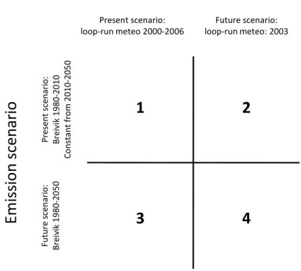
LOTOS-EUROS was run for the period 2000-2050, preceded by an initial running period for 1980-2000 to achieve realistic base line concentrations in the different environmental compartments at the start of the runs. Four runs were performed to study the absolute and relative effects of 1) changing climate conditions and 2) changing emissions on the environmental fate of PCB-153. This means that two sets of different climate input parameters were combined with two different emission input scenarios. In two of four runs (scenario 1 and 3), the actual meteorological/climate situation was simulated by looping the reported

meteorological situation of the years 2000-2006 (ECMWF; www.ecmwf.int). In the other two runs (scenario 2 and 4), as a surrogate of a meteorological scenario under possible future climate change conditions, the extremely warm

(12)

year 2003 was repeatedly applied. In both scenarios, the meteorological input data contained information on temperature, precipitation, wind field with a time resolution of three hourly intervals.

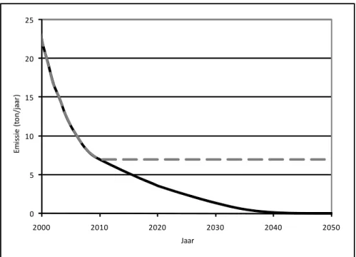
For the emissions, also two different scenarios were defined. All four runs use the emission inventory of Breivik et al. (2007) for the period 2000-2010 and the preceding initiation period (1980-1999). In two of four runs (scenario 1 and 2), it was subsequently assumed that from 2010 to 2050, the emissions would remain constant at the 2010 level. In the other two runs (scenario 3 and 4), future emissions as predicted by Breivik et al. (2007) were applied. They also developed indicative emission projections based on activity scenarios, in which the expected effects of the policy under the POP-Conventions were taken into account. The emissions in the two scenarios were put in the model as yearly averages. The four runs, with their combination of input scenarios, are given in Figure 2. As an indication, the average European emission levels for the period 2000-2050 in the two input scenarios are given in Figure 3.

Climate scenario

Emi

ssi

on

scenar

io

Presen t scen ar io: Breivik 1 980 ‐20 1 0 C o ns tant f rom 201 0 ‐20 5 0 Fu tu re sc en ar io : Brei vi k 1 980 ‐20 5 0 Present scenario: loop‐run meteo 2000‐2006 Future scenario: loop‐run meteo: 2003

1

2

4

3

Figure 2. Overview of the four combinations of climate input scenarios and emission scenarios run with LOTOS-EUROS.

The model outputs that were analyzed for this purpose, were the average concentrations of PCB-153 in air, sea water (upper layer) and soil in the modeling domain over the period 2000-2050, in order to study the overall time trends and their differences between the four scenarios. Also, the spatial distribution of the substance in air and soil was studied at different moments in time during the simulation period.

(13)

0 5 10 15 20 25 2000 2010 2020 2030 2040 2050 Em issi e (t o n /j aa r) Jaar

Figure 3. Total emissions of PCB-153 to air in the different emission scenarios. The black line represents the emission scenario of Breivik et al. (2007). The dotted line represents the scenario in which emissions remain constant between 2010 and 2050 on the 2010 level.

Table 1. The physical-chemical properties of PCB-153 used in this study.

Parameter Value Unit Reference

Molecular weight 361 g.mol-1 _{Mackay et al.,}

1992

Vapor pressure at 25˚C 8.8*10-5 _Pa _{Li et al., 2003} Water solubility at 25˚C 6.5*10-3_mg.l-1 _{Li et al., 2003}

Kow 1.4*107 - Li et al., 2003

Gas-water part. coefficient at 25˚C 2.1*10-3 _- _{Li et al., 2003} Solid-water part. coefficient at 25˚C 2.9*105 _- _{Li et al., 2003} Enthalpy of vaporization 8.8*101_kJ.mol-1_{Li et al., 2003} Enthalpy of dissolution 2.5*101_kJ.mol-1_{Li et al., 2003} Gas phase degradation rate

constant at 25˚C 3.5*10

-8 _s-1 _{Mackay et al.,} 1992

Dissolved phase degradation rate

constant at 25˚C 3.5*10

-9 _s-1 _{Mackay et al.,} 1992

Bulk degradation rate soil at 25˚C 3.5*10-9 _s-1 _{Mackay et al.,} 1992

(14)

3 Results

Average concentrations in air, soil and sea water over time

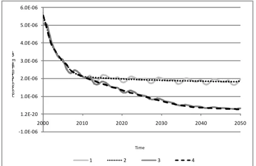
The predicted concentrations of PCB-153 in air from the year 2000 until the year 2050, averaged over the total model domain, are given in Figure 4. The

concentration time series are given for the four different climate-emission input scenarios (numbered as indicated in Figure 1). In general, concentrations are highest at the start of the simulation period; they drop quickly between 2000 and 2010, and show a smoother decline from 2010 until 2050. Up to the year 2010, all scenarios show similar concentration values, whereas between 2010 and 2050, the predicted concentrations for scenario 1 and 2, in which the emissions remain at the level of 2010 until 2050, are significantly higher than those of scenario 3 and 4 in which a decline in emissions was assumed as input. The differences between the two climate scenarios are less pronounced

(differences between scenario 1 and 2 and between scenario 3 and 4), although fluctuations between the years are larger in the 2000-2006 meteorological input compared to the 2003 input. The minimum to maximum air concentrations range from a factor of 7 below the average values up to a factor of 5 over the average values at the beginning of the modeling period, whereas at the end of the modeling period minimum and maximum concentrations are respectively about a factor of 2 and 3 lower and higher than the average. The air

concentrations show a close correlation with the emission levels.

‐1.0E‐06 1.2E‐20 1.0E‐06 2.0E‐06 3.0E‐06 4.0E‐06 5.0E‐06 6.0E‐06 2000 2010 2020 2030 2040 2050 1 2 3 4 C o n ce n tr at io n (µ g. m ‐3 ) Time

Figure 4. Average air concentrations (µg.m-3_{) in Europe in the four different}

scenarios over time (period 2000-2050).

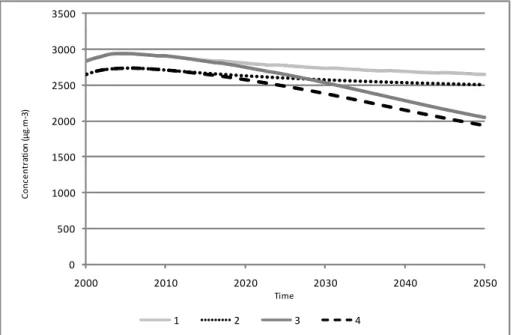
The predicted average soil concentrations in Europe between 2000 and 2050 in the four different scenarios are given in Figure 5. The soil concentrations show a different pattern in time than the air concentrations: they slightly increase up to 3000 µg.m-3_{in the first years of the simulation period until they reach}

equilibrium with the air concentrations, after which they slowly drop until the year 2050. The impact of emission change is also in soil higher than the impact of climate change, i.e. scenario 1 and 2 are more similar than scenario 3 and 4.

(15)

However, compared to the air compartment, the effects of changed climate parameters are a bit more pronounced in the soil compartment. I.e. assuming identical emissions, the scenarios in which a possible future climate was simulated show 7% lower predicted soil concentrations than the scenarios with the current climatological circumstances. The absolute lowering of average soil concentrations is caused by the fact that degradation of PCB-153 will proceed faster at higher temperatures.

0 500 1000 1500 2000 2500 3000 3500 2000 2010 2020 2030 2040 2050 1 2 3 4 Conc e n tr at io n (µ g.m ‐3) Time

Figure 5. Average soil concentrations (µg.m-3_{) in Europe in the four different}

scenarios over time (period 2000-2050).

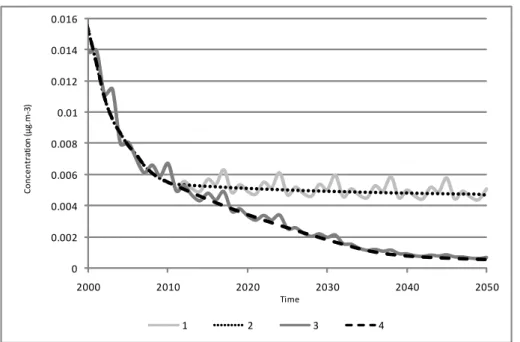
In the upper layer of the sea water compartment, the concentration patterns are comparable to the air concentration patterns (and thus to the emission

patterns), i.e. the concentrations in the upper part of the sea water react quicker to emission changes than the concentrations in soil (Figure 6). This is because volatilization from water as a reaction to declining emissions and air concentrations proceeds quicker in water than in soil, i.e. a new equilibrium with air is reached faster.

The concentration levels decline from about 0.015 µg.m-3_{in 2000 to 0.005} µg.m-3_{in 2010 in all four scenarios. In scenarios 1 and 2, the sea water levels} remain more or less constant after 2010 until 2050, whereas in scenario 3 and 4 they decline to a level of less than 0.001 µg.m-3_{between 2010 and 2050. This} means that as in the air compartment, in the sea water compartment the influence of the expected decline in emissions is of much more influence than the influence of a changed climate scenario. Minimum and maximum sea water concentrations are predicted to be about a factor of two lower resp. higher than the average concentrations throughout Europe (i.e. the total variation is a factor of 4).

(16)

0 0.002 0.004 0.006 0.008 0.01 0.012 0.014 0.016 2000 2010 2020 2030 2040 2050 1 2 3 4 Conc e n tr at io n (µ g.m ‐3) Time

Figure 6. Average sea water concentrations (µg.m-3_{) in Europe in the four}

different scenarios over time (period 2000-2050).

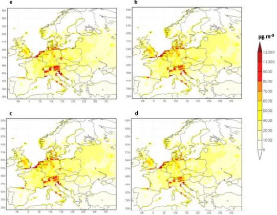
Spatial distribution of PCB-153 concentrations

In Figure 7, the European distribution of PCB-153 in the air in the year 2030 is shown for the four different scenarios. Figure 7a, 7b, 7c and 7d respectively represent scenarios 1, 2, 3 and 4. Figure 8 shows the PCB-concentrations that are predicted for the soil compartment. On the maps of both environmental compartments, it can be seen that there are differences in the absolute concentration values of PCB-153, but that the spatial patterns of the

concentrations are comparable, both in the different climate scenarios and in the emission scenarios. The highest concentration levels are found in North-West and Central Europe.

(17)

Figure 7. Predicted air concentrations of PCB-153 in Europe at mid 2030. 7a: scenario 1, 7b: scenario 2, 7c: scenario 3, 7d: scenario 4.

Figure 8. Predicted soil concentrations of PCB-153 in Europa at mid2030. 8a:

(18)

4 Discussion and conclusions

From the pilot study we performed here, it seems to appear that the expected effects of a changing climate on the distribution of PCB-153 in the environment during the next decennia will be much smaller than the expected effects of emission reductions, at least on an average European level. It must be noted, however, that in this study a fictive future climate scenario was applied, in which a relatively small raise of the average temperature and precipitation was

assumed with respect to some other climate scenarios that have been developed for the period until 2050. In reality, more or less severe temperature and

precipitation changes may occur, or other climatological circumstances may alter. It might therefore be valuable to perform a follow up study, similar to what was done here, but with more realistic future climate scenarios that are being developed by, i.e. the KNMI within the framework of the ‘Kennis voor Klimaat’ project.

Besides, climate change has effects on several environmental processes (Lamon et al., 2009b). Some were taken into account in the LE model, some were not. We looked at changes in wind speeds-POPs’ atmospheric distributions,

temperature-POPs’ degradation rates, precipitation-POPs’ wet deposition fluxes and volatilization. We neglected the effects of changing oceanic currents-POPs’ marine spatial distribution, ice cover-POPs’ release from ice, organic carbon content and vegetation mass-POPs’ absorption.

If we assume that the climate parameter changes used here are realistic, which we consider at least partly true, the following can be concluded: By the year 2050, the expected lowering of emissions may have led to 90% lower air concentrations and 20% lower soil concentrations compared to the situation in which the emissions will remain constant at the current level. The expected changes in concentrations in a future climate scenario on the other hand are much less pronounced, particularly in air and seawater: not more than 1-2% in these compartments. In the soil, the effects of a changing climate are expected to be larger: an average concentration drop of 7% is predicted for the year 2050. Further, from the current study, no clear shifts in the spatial distribution of PCB-153 were discovered; there are no big changes in emission patterns, neither do changing climate settings alter the spatial distribution of this substance.

Also from other existing studies appears that the effects of climate change, at least at continental and global scale levels, will not lead to drastic changes in the distribution of POPs’: Lamon et al. (2009a) for example, report concentration differences of a factor of 2 to 3 between current and future climate scenarios for PCB-153 and PCB-28 on a global level. Though, it might be possible that on local scale levels, more pronounced effects do appear, due to large local changes in environmental conditions, which are not accounted for on the European scale level applied in the current study (e.g due to local vegetation or land use changes). Besides, other POP compounds than PCBs might show different results.

Since, in this study, climate effects were weighed against the effects of changing emissions, it appears clearly that on a European level, the reduction in emissions is expected to have a relatively large effect on the concentration levels of PCB-153 compared to the climatic changes. And thus it can be concluded that the measures that have been taken to reduce these emissions will probably not be surpassed by opposite effects of climate change in one or more of the

environmental compartments. The latter seem to have even a slight positive effect on the PCB-concentrations, since degradation of PCB-153 will proceed faster at higher temperatures.

(19)

5 Part 2. A: Validation report LOTOS-EUROS – POP module

We performed a validation study to test the latest implementation of the POP module in the LOTOS-EUROS model (version1.5/patch025) for the substance PCB-153. We chose this substance, since an emission inventory for a sufficient period was available, as well as a number of measured concentration data in air, as well as soil and water. Moreover, for PCB-153, modeling studies (for the UK and the Northern Hemisphere) had been applied in the past using different models, of which the outcomes could be compared to the LOTOS-EUROS predictions as a second type of validation.

The LOTOS-EUROS run on which the validation was performed, was done for the period 1981-2000. As input, the emission inventory of Breivik et al. (2002; 2007) was used. The runs that were primarily selected for validation were runs 013, 014 and 016 (see Chapter 7 and Annex E, test runs with LE-POP), which reflect the most realistic meteorological scenario that could be performed with the available meteorological data (data from ECMWF; www.ecmwf.int). In run 013, zero boundary conditions were assumed, whereas in run 014 boundary conditions were assumed that were derived from the multimedia box model SimpleBox. Run 016 differs from runs 013 and 014 by the emission dataset that was used: For run 013 and 014, the dataset of Breivik et al. (2002) was applied, whereas for run 016 the updated emission dataset of Breivik et al. (2007) was used.

Air compartment

Comparison of LOTOS-EUROS predictions with EMEP measurement data

Parties to the Convention on Long-Range Transboundary Air Pollution (LRTAP) perform monitoring at regional monitoring sites across Europe. The data are subject to national quality assessments and are then submitted to the EMEP Chemical Coordinating Centre at NILU. The submitted data are further assessed by the EMEP-CCC in collaboration with the data originators and are reported on an annual basis on their website:

http://tarantula.nilu.no/projects/ccc/emepdata.html.

For air concentrations of PCB-153 in the period 1981-2000, the measurement data given in Table 1 of Annex A were available at EMEP (annual averages). The codes refer to measurement stations, of which the locations are indicated on the website of EMEP.

From the LE runs 013, 014 and 016, the annually averaged predicted air concentrations at these measurement locations were derived. The predicted concentrations of LE run 013 are given in Table 2a, those of LE run 014 are given in Table 2b and of run 016 in Table 2c of Annex A.

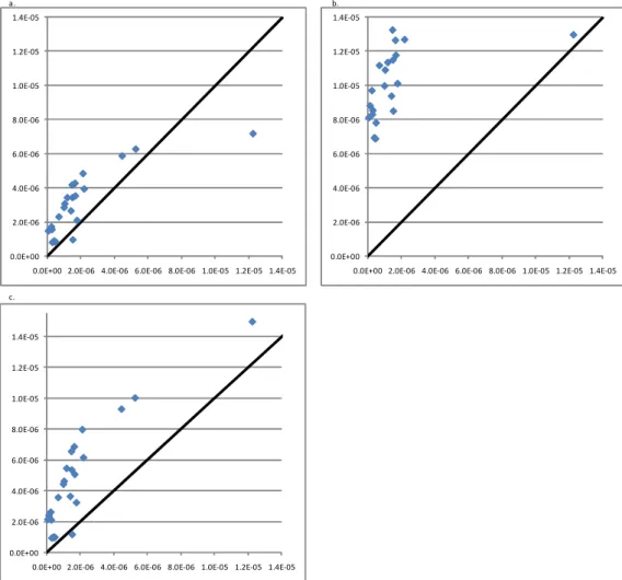
Both the modeled data (of run 013, 014 and 016), and the measured data were plotted in Figure 9a to Figure 9e, for each of the locations of the measurement stations separately. The ratios between the modeled and measured data in both runs are given in Table 2a, and the data were plotted against each other in scatter plots in Figure 10a (run 013), Figure 10b (run 014) and Figure 10c (run 016).

(20)

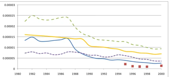
0 0.00001 0.00002 0.00003 0.00004 0.00005 0.00006 1980 1982 1984 1986 1988 1990 1992 1994 1996 1998 2000

Figure 9a. Predicted air concentrations by LE run 013 (blue line), LE run 014 (green dashed line) and LE run 016 (purple dotted line) in the period 1981-2000 at location of EMEP measurement station CZ0003R, and measured air

concentrations reported by EMEP (red dots) at the same location. Also modeled concentrations at this location by the MSCE-POP model are shown (orange line).

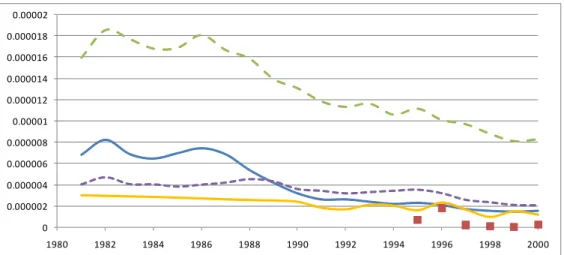
0 0.000002 0.000004 0.000006 0.000008 0.00001 0.000012 0.000014 0.000016 1980 1982 1984 1986 1988 1990 1992 1994 1996 1998 2000

Figure 9b. Predicted air concentrations by LE run 013 (blue line), LE run 014 (green dashed line) and LE run 016 (purple dotted line) in the period 1981-2000 at location of EMEP measurement station FI0096G, and measured air

(21)

0 0.000002 0.000004 0.000006 0.000008 0.00001 0.000012 0.000014 0.000016 0.000018 0.00002 1980 1982 1984 1986 1988 1990 1992 1994 1996 1998 2000

Figure 9c. Predicted air concentrations by LE run 013 (blue line), LE run 014 (green dashed line) and LE run 016 (purple dotted line) in the period 1981-2000 at location of EMEP measurement station IS0091R, and measured air

0 0.000005 0.00001 0.000015 0.00002 0.000025 0.00003 0.000035 0.00004 0.000045 1980 1982 1984 1986 1988 1990 1992 1994 1996 1998 2000

Figure 9d. Predicted air concentrations by LE run 013 (blue line), LE run 014 (green dashed line) and LE run 016 (purple dotted line) in the period 1981-2000 at location of EMEP measurement station SE0002R, and measured air

(22)

0 0.000005 0.00001 0.000015 0.00002 0.000025 0.00003 1980 1982 1984 1986 1988 1990 1992 1994 1996 1998 2000

Figure 9e. Predicted air concentrations by LE run 013 (blue line), LE run 014 (green dashed line) and LE run 016 (purple dotted line) in the period 1981-2000 at location of EMEP measurement station SE0012R, and measured air

Data point #1 #2 #3 #4 #5 #6 #7 #8 #9 #10 #11 #12

Run 013 0.59 0.31 0.63 2.64 1.69 1.88 2.26 3.36 1.18 7.08 11.79 23.08

Run 014 1.06 0.55 5.58 27.85 15.98 14.90 17.71 16.23 5.69 39.87 66.68 126.68

Run 016 1.22 0.64 0.76 3.05 2.02 2.11 2.52 5.19 1.83 10.77 18.13 33.53

Data point #13 #14 #15 #16 #17 #18 #19 #20 #21 #22 #23 #24 #25 min max average median

Run 013 5.71 1.19 1.32 2.28 2.83 2.60 2.29 2.11 1.80 2.89 2.95 2.86 1.89 0.31 23.08 3.57 2.28

Run 014 30.35 3.17 3.71 6.73 8.96 7.67 7.64 7.02 5.77 9.52 10.48 9.98 6.64 0.55 126.68 18.26 8.96

Run 016 7.72 1.90 2.09 3.75 4.44 4.17 3.57 3.03 2.80 4.59 4.45 4.44 2.58 0.64 33.53 5.25 3.05

Table 2a. The ratios between the air concentrations modeled by LE of run 013, run 014 and run 016 respectively, and the measured air concentrations.

(23)

a. b. c. 0.0E+00 2.0E‐06 4.0E‐06 6.0E‐06 8.0E‐06 1.0E‐05 1.2E‐05 1.4E‐05

0.0E+00 2.0E‐06 4.0E‐06 6.0E‐06 8.0E‐06 1.0E‐05 1.2E‐05 1.4E‐05

Figure 10. Scatter plots of the modeled air concentrations of LE (y-axis) for run 013 (Figure 10a), run 014 (Figure 10b) and run 016 (Figure 10c) against the measured air concentration data (x-axis) of EMEP.

From the Figures 9 and 10 and the tabulated measured:modeled air

concentration data in Table 2, it is clear that the modeled data of run 013 and run 016 show a good fit with the measured data, of which run 013 is generally the best. Except for two locations, the measured data are all within a factor of 6 from the modeled data of both runs, with a median measured:modeled ratio of 2.28 and 3.05 for run 013 and run 016 respectively. At one location, in Iceland (station IS0091R), the measured data show a large deviation from the modeled data in the years 1998-1999. Possibly, at that time, specific meteorological circumstances were present in Iceland that were not simulated in the

meteorological scenarios of the model runs. In the Figures 9-10 and Table 2, it is also shown that the deviation between measured and modeled air

concentrations for run 014 is much larger than for run 013 and run 016. In almost all cases, the model overestimates the air concentrations with about a factor of 10 (average ratio modeled:measured is 18.26, and the median ratio is 8.96). Obviously, the assumed boundary conditions (concentrations on the edges of the model domain) were estimated too high in run 014. This can be explained by the fact that these background concentrations were derived from a scenario in which European emissions were taken into account. Europe is by far the largest emission source of PCB-153, and largely account for the

concentrations outside Europe. By using the background concentrations derived following this scenario, and modeling European emissions again in LE, there is a kind of doubling of European emissions at the boundaries, which is not correct.

(24)

Based on the results of the validation of the modeled air concentrations and the measurement data, from which is clear that run 013 and run 016 perform very satisfactorily and much better than run 014, the remaining validation study was limited to comparison of measured and model data to LE run 013 and run 016.

Comparison of LOTOS-EUROS predictions with MSCE-POP predictions

The Meteorological Synthesizing Centre East (MSC-E) performs model

calculations on POP concentrations for EMEP. For that goal, they use their own MSCE-POP model. This model was also run for PCB-153 concentrations in the period 1980-2000, making use of the emission estimates of Breivik (2007). The predicted air concentrations on the selected EMEP measurement locations by the MSCE-POP model are plotted with orange lines in Figures 9a to 9e. The ratios between the modeled concentrations by LOTOS-EUROS runs 013 and 016 respectively and the MSCE-POP run (on an annual average basis) are given in Table 2b.

For run 013, the ratios between the LOTOS-EUROS model and the MSCE-POP model are between a factor of 1.0 to 3.7, with an average ratio of 1.96. For run 016, the ratios between the LOTOS-EUROS model and the MSCE-POP model are between a factor of 1.3 to 3.4, with an average ratio of 1.84. In most cases, the MSCE-POP concentrations are predicted to be higher than the LOTOS-EUROS calculations, except for location IS0091R. At this location, the MSCE-POP model also closely corresponds with the measurement data of EMEP, whereas at almost all other locations, the LOTOS-EUROS model shows better agreement with the measurement data (both runs 013 and 016).

ratio MSCE‐POP/LE run 013 ratio MSCE‐POP/LE run 016

CZ3 FI96 IS91 SE2 SE12 CZ3 FI96 IS91 SE2 SE12

1981 1.4 1.3 0.4 0.8 1.2 1981 1.8 2.5 0.7 1.8 2.2 1982 1.4 1.4 0.4 0.8 1.1 1982 1.8 2.9 0.6 1.7 2.0 1983 1.6 1.7 0.4 0.9 1.2 1983 1.8 3.4 0.7 1.9 2.2 1984 1.6 1.5 0.4 0.8 1.2 1984 1.7 2.9 0.7 1.7 2.1 1985 1.3 1.3 0.4 0.8 1.1 1985 1.8 2.7 0.7 2.0 2.3 1986 1.4 1.2 0.4 0.8 1.1 1986 1.8 2.5 0.7 1.9 2.1 1987 1.4 1.4 0.4 0.7 1.0 1987 1.7 2.6 0.6 1.5 1.8 1988 1.9 1.8 0.5 1.1 1.5 1988 1.6 2.2 0.6 1.5 1.8 1989 1.5 2.5 0.6 1.6 2.0 1989 1.7 2.8 0.6 1.7 1.9 1990 1.1 2.4 0.8 1.8 1.9 1990 1.5 2.5 0.7 1.6 1.7 1991 2.3 2.7 0.7 1.9 2.1 1991 1.7 2.6 0.5 1.4 1.6 1992 2.4 2.2 0.7 2.0 2.1 1992 1.7 2.1 0.5 1.7 1.8 1993 3.1 2.4 0.9 2.2 2.3 1993 1.6 2.0 0.6 1.6 1.7 1994 3.1 2.6 0.9 2.0 2.2 1994 1.7 2.1 0.6 1.3 1.4 1995 3.0 2.0 0.7 2.1 2.1 1995 1.5 1.5 0.5 1.3 1.3 1996 3.4 2.8 1.1 2.2 2.3 1996 1.6 2.3 0.7 1.4 1.5 1997 3.7 2.7 1.0 2.8 2.4 1997 1.6 2.3 0.6 1.8 1.6 1998 3.5 2.7 0.7 2.4 2.6 1998 1.6 2.2 0.4 1.5 1.6 1999 3.4 2.7 1.0 2.8 2.7 1999 1.6 2.4 0.7 1.8 1.8 2000 3.4 2.5 0.8 2.6 2.6 2000 1.7 2.3 0.6 1.8 1.9

Table 2b. The ratios between the modeled air concentrations by LOTOS-EUROS runs 013 and 016 respectively and the MSCE-POP run (on an annual average basis).

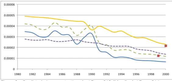
Validation against modeled data of Sweetman and Jones (1999)

Sweetman and Jones (1999) modeled concentrations of PCB-153 in air, water, soil and sediment in the UK for the period 1930-2000. The reported values for the period 1981-2000 in air were compared to those of LE run 013 and run 016 and plotted in Figure 11. In general, the modeled data of Sweetman and Jones are somewhat lower than those of LE run 013 in the period 1980-1992 (month 1-150), and both models fit well in the latest period (1992-2000). On the

(25)

contrary, LE run 016 predicts lower air concentrations over the period 1980-1992 than Sweetman, whereas the concentrations in the period 1980-1992-2000 are somewhat overestimated by this LE run. However, the emission data used by Sweetman and Jones (1999) were primarily derived from UK production amounts, and not from the dataset of Breivik et al. (2007) as in the LE-runs, which may cause some mismatches in the predicted concentrations. It can further be seen that in the LE modeling study, seasonal variations are not accounted for, whereas they are in the study of Sweetman and Jones. In Table 3, the modeled air concentrations of both models are given at a 2.5 year interval, with yearly averaged values, as well as the ratio between the modeled values. The predicted air concentrations in both models deviate in almost all cases less than a factor of 2.5, and most even within a factor of 2. The largest deviation between Sweetman and LE is shown for 1988 in LE run 013: here both model outputs differ a factor of 4. Over all, LE run 016 performs slightly more consistent with the model of Sweetman than LE run 013.

0.00E+00 2.00E‐05 4.00E‐05 6.00E‐05 8.00E‐05 1.00E‐04 1.20E‐04 1.40E‐04 1.60E‐04 1 51 101 151 201

Sweetman run 013 run 016

Figure 11. Modeled air concentrations of PCB-153 with LE run 013 (green line), LE run 016 (blue line) and the model of Sweetman and Jones (1999; red line) in the period 1981-2000 (month 1-240).

Year Sweetman LE run 013 LE run 016 Ratio 013/SW % Difference Ratio 016/SW % Difference

1981 4.60E‐05 3.93E‐05 1.92E‐05 0.85 ‐14.62% 0.42 ‐58.19%

1983 3.30E‐05 7.40E‐05 2.11E‐05 2.24 124.26% 0.64 ‐36.07%

1985 2.30E‐05 3.33E‐05 1.78E‐05 1.45 44.90% 0.77 ‐22.76%

1988 1.60E‐05 6.61E‐05 1.81E‐05 4.13 312.94% 1.13 13.04%

1990 1.20E‐05 2.14E‐05 1.66E‐05 1.78 78.40% 1.38 38.38%

1993 8.00E‐06 1.11E‐05 1.53E‐05 1.38 38.26% 1.92 91.68%

1995 6.00E‐06 1.13E‐05 1.27E‐05 1.89 88.77% 2.12 111.96%

1998 4.00E‐06 6.89E‐06 1.01E‐05 1.72 72.17% 2.52 151.53%

2000 2.50E‐06 5.32E‐06 6.58E‐06 2.13 112.99% 2.63 163.36%

average 1.95 95.34% 1.50 50.33%

median 1.78 78.40% 1.38 38.38%

Table 3. Modeled air concentrations with the model of Sweetman and Jones (1999) and LE run 013 and run 016, and the ratio between the modeled values.

(26)

Soil compartment

Measured concentrations of Meijer et al. (2003)

Measured soil concentration data throughout Europe were available from Meijer et al., 2003. The measured data were all from the year 1998, measured in both agricultural and rural soils. The 77 measurement locations and the

corresponding measured concentrations pg.g-1_{are given in Annex B. Also the} modeled concentrations by LE run 013 and LE run 016, averaged over the year 1998 at the same locations are given in this table, as well as the ratio between modeled and measured soil concentrations. The same data plotted in scatter plots in Figure 12. In the runs of LE, no distinction was made between

agricultural and rural soils, and so similar concentrations were predicted for both types of soils.

From Figure 12, it can be concluded that soil concentrations modeled by LE run 013 and run 016 are almost all within one order of magnitude from the

measured soil concentrations. In run 013, the model has the tendency to

overestimate the soil concentrations (a relatively large amount of dots are above the 1:1-line), whereas in run 016 the number of locations with overestimated concentrations is close to the number of underestimated concentrations. Although the deviations between measured and modeled concentrations are larger in the soil compartment than in the air compartment, the predicted soil concentrations are considered reliable. This is, because in the soil compartment conditions and concentrations can differ largely over very short distances. This is i.e. reflected in the list of measured concentrations: even at locations that are within the same grid cell, concentrations of PCB-153 were measured differing more than 1 order of magnitude. Such local variations are not being modeled in LE, so predicting ‘average’ concentrations that deviate less than the local soil variations differ among each other implies that the model, with the spatial resolution it has, performs adequately.

From the soil samples of which PCB-153 concentrations were measured, also the organic carbon content was known as single indication of the local conditions. This parameter was fit in the scatter plot of Figure 13, in order to see if a relationship exists between the soil organic carbon content and the measured soil concentrations. From Figure 14 it can be seen that there is no clear relationship (R2_{= 0.06).} a. b. 1 10 100 1000 10000 1 10 100 1000 10000

Measured (x) vs Modeled (y) 1:1 y=10x y=0.1x

1 10 100 1000 10000 1 10 100 1000 10000

Measured (x) vs Modeled (y) 1:1 y=10x y=0.1x

Figure 12. Scatter plot of the measured soil concentrations of Meijer et al. (2003) and the modeled soil concentrations by LE run 013 (Figure 4a) and LE

(27)

R² = 0.0639 0 2000 4000 6000 8000 10000 12000 14000 16000 18000 20000 0 10 20 30 40 50 60 70 80 90 100

Figure 13: Soil organic carbon content (x-axis) versus measured soil concentrations of Meijer et al.

Inland water concentrations

Validation against modeled data of Sweetman and Jones (1999)

From the study of Sweetman and Jones (1999), modeled fresh water

concentrations in the UK were available for the period 1930-2000. The modeled water concentrations for the period 1980-2000 are given by the blue line in Figure 14 in pg.l-1_.

LE runs 013 and 016 do not make any distinction between fresh water and sea water concentrations, all water bodies are considered equal. The modeled water concentrations in the UK (averaged over 20 different UK locations) for the period 1981-2000 by LE run 013 are given by the red line in Figure 16 and in Table 4 in pg.l-1_.

In both models, there is a trend of declining concentrations of PCB-153 during the modeling episode. LE run 013 predicts significantly higher concentrations in the first part of the modeling period (1980-1993), whereas in the period 1993-2000, the predicted water concentrations of both models are close to each other: they don’t deviate more than a factor 1.9. LE run 016 predictions are in general closer to those of Sweetman, however there is some overestimation during the total modeling period. The average ratio between the outcomes of run 013 and those of Sweetman is 2.1, and between the values of run 016 and Sweetman it is 1.9 over the full modeling period. In LE, some seasonal and interannual variations were modeled, which were absent in the model of Sweetman and Jones.

(28)

0 10 20 30 40 50 60 70 80 1982 1987 1992 1997

Figure 14. Modeled fresh water concentrations by Sweetman and Jones (1999; blue line) for the period 1980-2000, and by LE run 013 (green line) and LE run

016 (red line) in the UK. Values are in pg.l-1_.

Sweetman LE run 013 ratio LE run 016 ratio pg.l‐1 pg.l‐1 pg.l‐1 1980 dec 23 39.02537 1.7 1.46E+01 0.6 1983 jun 19 59.46634 3.1 2.29E+01 1.2 1985 dec 17 56.16977 3.3 2.21E+01 1.3 1988 jun 14 34.38237 2.5 1.63E+01 1.2 1990 dec 11.5 28.05775 2.4 1.99E+01 1.7 1993 jun 8 11.80404 1.5 1.57E+01 2.0 1995 dec 6 6.245007 1.0 1.31E+01 2.2 1998 jun 4 7.781348 1.9 1.66E+01 4.2 2000 dec 3 4.469493 1.5 9.22E+00 3.1 Average 2.1 1.9

Table 4. Modeled fresh water concentrations by Sweetman and Jones (1999) for the period 1980-2000, and by LE run 013 and run 016 and LE run 016 in the UK.

(29)

6 Part 2. B: LOTOS-EUROS test report POP module v1.5.025

Introduction

One of the options for the chemical transport code LOTOS-EUROS, is to use it for the transport of POP (Persistent Organic Pollutant). However, the POP module of LOTOS-EUROS had not been used since 2007 (e.g. Hollander et al., 2007) and the source code had not been updated for several years. It was decided to implement the POP module into one of the newest versions of LOTOS-EUROS: v1.5/patch025. This test-report describes the changes that had to be made and several tests that have been performed for the new LOTOS-EUROS version. Changes

The most important change that had to be made was the implementation of a new land use database (CORINE land cover database, see Smiatek (1998)). Test set up

Test runs were performed simulating PCB-153 transport during 1981-2000. Emissions were derived from Breivik et al. (2002; 2007). Since not all

meteorological data was readily available, it was decided to use the meteo-data from the period 2000 – 2006 (in different combinations, see below) during the simulation period.

Compiler options

Results of runs 003 and 004 with different compiler options fast (-O3) and check (-g –Check=all) resp. were compared. The simulation was only run for the year 1981. The resulting hourly values of several parameters showed some

differences in the order of rounding errors < 0.1 % or less. As a typical example, we show the difference in terms of percentage between the two runs for the concentration in the upper soil layer.

Figure 15. Difference (%) between runs with fast and check compiler options for concentration in upper soil layer, first year (1981).

Monthly averages for November 1981 showed also differences in the order of 0.01 % or less. Only for ddup (upward dry deposition), relative differences were ~ 1.5%, but absolute differences were in the order of 10-8_kg/month.

(30)

Bug in pop_aerosolsurf

In subroutine pop_aerosolsurf, the aerosol surface is computed. Mass fractions fi

and median diameters Di are defined for 5 different size classes:

DATA fr/ 0.42, 0.33, 0.14, 0.6 , 0.5 , & ! PAH's

0.70, 0.20, 0.5 , 0.3 , 0.2 , & ! pesticide

0.70, 0.20, 0.5 , 0.3 , 0.2 / ! other

DATA md/ 0.2 , 1.5 , 6.0 ,14.0 ,40.0 /

The mass fractions do not sum to 1, because an error has been made when transferring percentages into fractions. The correct data are:

DATA fr /0.42, 0.33, 0.14, 0.06, 0.05, & ! PAH's

0.70, 0.20, 0.05, 0.03, 0.02, & ! pesticide

0.70, 0.20, 0.05, 0.03, 0.02 / ! other

The relevant parameter in the computations here is

_

i i D

f _{. Fortunately, the} classes with incorrect mass fractions do not contribute much to the sum, because of the relatively high values of the diameter. The very small effect of this bug on the ratio of (particle mass)/(total mass) for different types of POP's (as computed in routine pop_calcrpg), can be seen in Figure 16. The effect on a LOTOS-EUROS run is negligible (< 0.1% for air concentrations, < 0.2% for upper soil layer concentrations in 2000).

Figure 16: Ratio (particle mass)/(total mass) for PAH, pesticide and other type of POP, with and without bug in pop_aerosolsurf. The asterisks show data from Van Jaarsveld (1995), section 6.3.3.1. The deviation for the pesticide γ-HCH is mainly due to a difference in vapor pressure between LOTOS-EUROS and van Jaarsveld.

The ratio particle/(total mass) for a LOTOS-EUROS run for PCB_153 is shown in Figure 17.

(31)

Figure 17: Ratio (particle mass)/(total mass) for PCB-153, meteo from year

2000. A PM concentration of 30 µg/m3_{is assumed. The red line indicates the}

mean ratio over 2000.

Meteo

Since not all meteo years in the simulation period 1981-2000 are currently available, LOTOS-EUROS runs with 'recycled' meteo. Different distributions of meteo years have been tested:

a. run006: meteo from 2000 – 2006; different meteo years are distributed over the simulation years, taking care that leap years in the simulation period coincide with leap years in the meteo years (2000, 2004). The following mapping has been used:

1981 1982 1983 1984 1985 1986 1987 1988 1989 1990 1991 1992 1993 1994 1995 1996 1997 1998 1999 2000 2001 2002 2003 2004 2005 2006 2001 2000 2002 2003 2005 2004 2006 2001 2002 2004 2003 2005 2006 2000 b. run007: meteo 2000 c. run008: meteo 2004

d. run013: meteo 2000 – 2006 in sequence; meteo for leap day is repeat of February 28 (if leap day in meteo year is not available).

(32)

Figure 18: PCB-153 concentration in upper soil layer, for different grid cells in Europe. While the concentration in Southern Europe (Spain) decreases in the '90s, the concentration in Northern parts of Europe (Sweden) still increases. Differences between individual meteo years can be significant (e.g. run 007 vs. 008). The order of the meteo years 2000-2006 does not have much effect (run 006 vs. 013).

(33)

Figure 19: soil concentration in Europe, agricultural land, average over Dec. 1999 – Nov. 2000. Panels show results of run 006, run 013 (which differ only in the order of the meteo years used), and the absolute and relative difference between these runs. The order of the meteo years used (2000-2006) does not have much effect; relative differences are only a few percent.

Figure 20: soil concentration in Europe, agricultural land, average over Dec. 1999 – Nov. 2000. Panels show results of run 007 (meteo 2000), run 008 (meteo 2004), the absolute and relative difference between these runs. The use of individual meteo years has a rather large impact.

(34)

Figure 21: air concentration in Europe, average over Dec. 1999 – Nov. 2000. Panels show results of run 006, run 013 (which differ only in the order of the meteo years used), the absolute and relative difference between these runs. The order of the meteo years used (2000-2006) has a larger effect on air

concentrations than on soil concentrations (as shown in Figure 5); in large parts of Europe, relative differences can amount to 20%.

Conclusions:

- the use of individual meteo years can have a large impact on PCB-153 concentrations.

- If the order of the meteo years inside a set of meteo years (2000-2006) is changed (runs 006 and 013), air concentrations for a specific year can change by 20%.

- For soil concentrations, the effect of changing the order of meteo years was much less (< 5%).

- Averaging over 7 years implies that differences between runs 006 and 013 decrease (< 10%), whereas differences between runs 007 (meteo 2000) and 008 (meteo 2004) over a 7-year averaging period can still be as large as 50% in certain parts of Europe.

- The set-up of run013 (meteo 2000 – 2006 in sequence; meteo for leap day is repeat of February 28, if leap day in meteo year is not available) is probably the most realistic and will be used in future runs.

(35)

Horizontal diffusion and advection

Recently, it has been recognized that LOTOS-EUROS has the tendency to

overestimate horizontal diffusion. To check what the effect of this overestimation can be, run010 was performed with horizontal diffusion switched off. A

comparison between this run and the base run008 (with horizontal diffusion) is presented in Figure 8:

Figure 8: air concentration of PCB-153, average over Dec. 1999 – Nov. 2000. Effect of switching off horizontal diffusion in run010 is limited to some localized differences of more than 10%.

Another comparison has been made between two different advection schemes: the standard Walcek scheme (run008, Walcek (2000)) and the κ = ⅓ scheme (run009; Van Leer, 1985). The latter scheme was present in LOTOS-EUROS but has not been used for years.

(36)

Figure 9: air concentration of PCB-153, average over Dec. 1999 – Nov. 2000. The Walcek scheme (run008) gives 20-40% higher concentration than the κ = ⅓ scheme (run009).

Boundary conditions

The effect of applying boundary conditions, derived from a global model (SimpleBox global scale), on the lateral boundaries of the model domain is investigated in run014.

Figure 10: PCB-153 concentration in upper soil layer, for different grid cells in Europe. Using a zero boundary condition (run013) or boundary conditions from a global model (run014).

(37)

Figure 11: PCB-153 soil concentration in Europe, agricultural land, average over Dec. 1999 – Nov. 2000. Panels show results of run 013 (zero boundary

conditions) and run 014 (boundary conditions from global model), the absolute and relative difference between these runs.

Figure 12: PCB-153 air concentration in Europe, average over Dec. 1999 – Nov. 2000. Panels show results of run 013 (zero boundary conditions) and run 014 (boundary conditions from global model), the absolute and relative difference between these runs.

(38)

Conclusions:

- concentrations in both soil and air increase due to boundary conditions; in continental Western Europe by 20 – 100%.

- The increase in concentrations is much higher in North-Western Europe and it shows a North-West (high) to South-East (low) gradient. At the outer Southern and Eastern edges there is again a higher increase.

(39)

7 References

 Breivik K, Sweetman A, Pacyna JM, Jones KC, 2002. Towards a global historical emission inventory for selected PCB congeners – a mass balance approach. 2. Emissions. Science of the Total Environment. Vol. 290 (1-3): 199-224.

 Breivik K, Sweetman A, Pacyna JM, Jones KC, 2007. Towards a global historical emission inventory for selected PCB congeners – a mass balance approach. 3. An update. Science of the Total Environment. Vol. 377 (2-3): 296-307.

 Dalla Valle, M., Codato, E. & Marcomini, A., 2007. Climate change influence on POPs distribution and fate: A case study. Chemosphere, 67 (7): 1287-1295.

 EMEP, 2010. EMEP measurement data online: http://tarantula.nilu.no/projects/ccc/emepdata.html.

 Hedegaard, G.B., Brandt, J., Christensen, J.H., Frohn, L.M., Geels, C., Hansen, K.M. & Stendel, M., 2008. Impacts of climate change on air pollution levels in the Northern Hemisphere with special focus on Europe and the Arctic. Atmospheric Chemistry and Physics, 8 (12): 3337-3367.  Hollander, A., Sauter, F., Den Hollander, H., Huijbregts M., Ragas, A.,

Van de Meent, D., 2007. Spatial variance in multimedia mass balance models: Comparison of LOTOS–EUROS and SimpleBox for PCB-153. Chemosphere 68 1318–1326.

 Jacobs CMJ, Van Pul WAJ, 1996. Long-range atmospheric transport of persistent organic pollutants. I: Description of surface-atmosphere exchange modules in implementation in EUROS. National Institute of Public Health and the Environment (RIVM) report number 7322401013. Bilthoven, The Netherlands.

 Lamon, L., von Waldow, H., MacLeod, M., Scheringer, M., Marcomini, A. & Hungerbuhler, K., 2009a. Modeling the Global Levels and Distribution of Polychlorinated Biphenyls in Air under a Climate Change Scenario. Environmental Science & Technology, 43 (15): 5818-5824.

 Lamon, L., Valle, M.D., Critto, A. & Marcomini, A., 2009b. Introducing an integrated climate change perspective in POPs modelling, monitoring and regulation. Environmental Pollution, 157 (7): 1971-1980.

 Macleod, M., Riley, W.J., McKone, T.S., 2005. Assessing the influence of climate variability on atmospheric concentrations of polychlorinated biphenyls using a global-scale mass balance model (BETR-Global). Environ. Sci. Technol. 39, 6749–6756.

 Meijer SN, Ockenden WA, Sweetman A, Breivik K, Grimalt JO, Jones KC, 2003. Global distribution and budget of PCBs and HCB in background surface soils: Implications for sources and environmental processes. Environmental Science and Technology 37: 667-672.

 Schaap, M.,Timmermans, R.M.A., Roemer, M., Boersen, G.A.C., Builtjes, P.J.H., Sauter, F.J., Velders, G.J.M. and Beck, J.P. (2008) ‘The LOTOS– EUROS model: description, validation and latest developments’, Int. J. Environment and Pollution, Vol. 32, No. 2, pp.270–290.

 Sweetman AJ, Jones KC, 1999. Modelling historical emissions and environmental fate of PCBs in the UK. PERSISTENT, BIOACCUMULATIVE, TOXIC CHEMICALS; Persistence and Modeling. Symposia Papers.

Presented Before the Division of Environmental Chemistry American Chemical Society. Anaheim, CA March 21-25, 1999.

(40)

8 Annexes

Annex A. Measured and modeled air concentrations

Table 1. Available measured air concentrations of EMEP in the period 1981-2000 (annual averages).

CZ0003R DE0001R FI0096G GB0014R IS0091R NO0001R NO0042G SE0002R SE0012R SE0014R

ug/m3 ug/m3 ug/m3 ug/m3 ug/m3 ug/m3 ug/m3 ug/m3 ug/m3 ug/m3 1981

1982 1983 1984 1985 1986 1987 1988 1989 1990 1991 1992 1993 5.27E‐06 1994

6.87E‐07 4.46E‐06 2.19E‐06 1995

1.52E‐06 1.77E‐06 2.13E‐06 1.19E‐06 1996

3.06E‐07 2.43E‐07 1.48E‐06 1.04E‐06 1997

4.88E‐07 1.32E‐07 6.26E‐07 1.65E‐06 9.98E‐07 1998

1.23E‐05 4.61E‐07 6.40E‐08 1.03E‐06 1.50E‐06 1999

2.15E‐05 3.91E‐07 2.73E‐07 3.95E‐07 1.67E‐06 1.41E‐06 2000

Table 2a. Predicted air concentrations of LE run 013 (annual averages) at the locations of the measurement stations of EMEP.

ug/m3 ug/m3 ug/m3 ug/m3 ug/m3 ug/m3 ug/m3 ug/m3 ug/m3 ug/m3

3.47E‐05 6.41E‐05 3.85E‐06 5.25E‐05 6.82E‐06 1.75E‐05 ‐9.90E+01 2.53E‐05 1.33E‐05 2.55E‐05 1981

3.36E‐05 7.44E‐05 3.54E‐06 6.11E‐05 8.21E‐06 1.82E‐05 ‐9.90E+01 2.67E‐05 1.48E‐05 2.69E‐05 1982

3.00E‐05 7.16E‐05 2.94E‐06 5.82E‐05 6.88E‐06 1.63E‐05 ‐9.90E+01 2.19E‐05 1.30E‐05 2.21E‐05 1983

3.00E‐05 7.96E‐05 3.17E‐06 6.20E‐05 6.45E‐06 1.89E‐05 ‐9.90E+01 2.49E‐05 1.29E‐05 2.51E‐05 1984

3.54E‐05 7.25E‐05 3.70E‐06 5.85E‐05 6.96E‐06 1.64E‐05 ‐9.90E+01 2.36E‐05 1.33E‐05 2.38E‐05 1985

3.19E‐05 7.00E‐05 3.75E‐06 4.98E‐05 7.43E‐06 1.55E‐05 ‐9.90E+01 2.34E‐05 1.36E‐05 2.35E‐05 1986

3.14E‐05 6.89E‐05 3.27E‐06 5.58E‐05 6.86E‐06 1.85E‐05 ‐9.90E+01 2.68E‐05 1.41E‐05 2.70E‐05 1987

2.31E‐05 2.74E‐05 2.44E‐06 3.61E‐05 5.37E‐06 1.22E‐05 ‐9.90E+01 1.61E‐05 9.21E‐06 1.61E‐05 1988

2.93E‐05 2.32E‐05 1.71E‐06 3.40E‐05 4.19E‐06 8.65E‐06 ‐9.90E+01 1.13E‐05 7.01E‐06 1.14E‐05 1989

3.29E‐05 2.04E‐05 1.37E‐06 2.49E‐05 3.19E‐06 6.74E‐06 ‐9.90E+01 8.19E‐06 5.69E‐06 8.22E‐06 1990

1.76E‐05 2.00E‐05 1.31E‐06 2.00E‐05 2.63E‐06 6.25E‐06 ‐9.90E+01 7.68E‐06 4.87E‐06 7.71E‐06 1991

1.56E‐05 1.78E‐05 1.37E‐06 3.20E‐05 2.63E‐06 5.69E‐06 ‐9.90E+01 7.11E‐06 4.72E‐06 7.13E‐06 1992

1.10E‐05 1.45E‐05 1.25E‐06 8.91E‐06 2.41E‐06 4.12E‐06 ‐9.90E+01 5.82E‐06 4.10E‐06 5.84E‐06 1993

1.12E‐05 1.46E‐05 1.09E‐06 8.78E‐06 2.21E‐06 4.48E‐06 ‐9.90E+01 6.28E‐06 4.26E‐06 6.31E‐06 1994

1.05E‐05 1.27E‐05 1.22E‐06 6.88E‐06 2.31E‐06 4.21E‐06 ‐9.90E+01 5.88E‐06 3.95E‐06 5.90E‐06 1995

8.47E‐06 1.20E‐05 9.60E‐07 7.10E‐06 2.10E‐06 3.52E‐06 ‐9.90E+01 4.85E‐06 3.43E‐06 4.86E‐06 1996

7.94E‐06 1.12E‐05 8.07E‐07 6.83E‐06 1.72E‐06 3.23E‐06 ‐9.90E+01 4.18E‐06 3.07E‐06 4.19E‐06 1997

7.76E‐06 1.15E‐05 8.24E‐07 6.94E‐06 1.56E‐06 3.40E‐06 ‐9.90E+01 4.28E‐06 2.85E‐06 4.30E‐06 1998

7.19E‐06 8.83E‐06 8.65E‐07 5.41E‐06 1.48E‐06 2.57E‐06 ‐9.90E+01 3.44E‐06 2.53E‐06 3.44E‐06 1999

(41)

Table 2b. Predicted air concentrations of LE run 014 (annual averages) at the locations of the measurement stations of EMEP.

4.20E‐05 7.65E‐05 1.31E‐05 6.65E‐05 1.59E‐05 2.89E‐05 ‐9.90E+01 3.61E‐05 2.23E‐05 3.62E‐05 1981

4.09E‐05 8.93E‐05 1.34E‐05 7.75E‐05 1.85E‐05 3.10E‐05 ‐9.90E+01 3.93E‐05 2.50E‐05 3.94E‐05 1982

3.72E‐05 8.59E‐05 1.34E‐05 7.40E‐05 1.77E‐05 2.90E‐05 ‐9.90E+01 3.42E‐05 2.34E‐05 3.44E‐05 1983

3.73E‐05 9.36E‐05 1.31E‐05 7.79E‐05 1.68E‐05 3.17E‐05 ‐9.90E+01 3.70E‐05 2.28E‐05 3.72E‐05 1984

4.31E‐05 8.72E‐05 1.26E‐05 7.48E‐05 1.69E‐05 2.92E‐05 ‐9.90E+01 3.60E‐05 2.32E‐05 3.61E‐05 1985

3.90E‐05 8.53E‐05 1.33E‐05 6.59E‐05 1.81E‐05 2.90E‐05 ‐9.90E+01 3.66E‐05 2.40E‐05 3.67E‐05 1986

3.87E‐05 8.30E‐05 1.26E‐05 7.16E‐05 1.67E‐05 3.14E‐05 ‐9.90E+01 3.92E‐05 2.39E‐05 3.94E‐05 1987

3.12E‐05 4.17E‐05 1.18E‐05 5.15E‐05 1.58E‐05 2.58E‐05 ‐9.90E+01 2.89E‐05 1.95E‐05 2.90E‐05 1988

3.67E‐05 3.67E‐05 1.09E‐05 4.91E‐05 1.39E‐05 2.07E‐05 ‐9.90E+01 2.29E‐05 1.65E‐05 2.30E‐05 1989

4.03E‐05 3.31E‐05 1.10E‐05 3.90E‐05 1.31E‐05 1.84E‐05 ‐9.90E+01 1.94E‐05 1.53E‐05 1.94E‐05 1990

2.47E‐05 3.19E‐05 1.02E‐05 3.37E‐05 1.18E‐05 1.75E‐05 ‐9.90E+01 1.82E‐05 1.38E‐05 1.83E‐05 1991

2.27E‐05 3.01E‐05 9.28E‐06 4.61E‐05 1.13E‐05 1.69E‐05 ‐9.90E+01 1.77E‐05 1.34E‐05 1.77E‐05 1992

1.76E‐05 2.72E‐05 9.61E‐06 2.23E‐05 1.16E‐05 1.57E‐05 ‐9.90E+01 1.70E‐05 1.31E‐05 1.71E‐05 1993

1.79E‐05 2.62E‐05 9.17E‐06 2.15E‐05 1.06E‐05 1.55E‐05 ‐9.90E+01 1.67E‐05 1.28E‐05 1.68E‐05 1994

1.78E‐05 2.46E‐05 9.12E‐06 1.93E‐05 1.12E‐05 1.55E‐05 ‐9.90E+01 1.66E‐05 1.27E‐05 1.66E‐05 1995

1.49E‐05 2.30E‐05 8.49E‐06 1.90E‐05 1.01E‐05 1.34E‐05 ‐9.90E+01 1.43E‐05 1.13E‐05 1.43E‐05 1996

1.41E‐05 2.13E‐05 8.52E‐06 1.78E‐05 9.69E‐06 1.27E‐05 ‐9.90E+01 1.32E‐05 1.09E‐05 1.33E‐05 1997

1.37E‐05 2.09E‐05 7.80E‐06 1.74E‐05 8.80E‐06 1.24E‐05 ‐9.90E+01 1.26E‐05 9.96E‐06 1.26E‐05 1998

1.29E‐05 1.81E‐05 6.87E‐06 1.57E‐05 8.11E‐06 1.12E‐05 ‐9.90E+01 1.15E‐05 9.25E‐06 1.15E‐05 1999

1.18E‐05 1.78E‐05 6.92E‐06 1.39E‐05 8.29E‐06 1.11E‐05 ‐9.90E+01 1.17E‐05 9.36E‐06 1.18E‐05 2000

Table 2c. Predicted air concentrations of LE run 016 (annual averages) at the locations of the measurement stations of EMEP.

2.79E‐05 1.99E‐05 1.98E‐06 1.87E‐05 4.08E‐06 7.55E‐06 ‐9.90E+01 1.18E‐05 7.37E‐06 1.18E‐05 1981

2.69E‐05 2.21E‐05 1.70E‐06 1.98E‐05 4.73E‐06 7.62E‐06 ‐9.90E+01 1.21E‐05 7.94E‐06 1.22E‐05 1982

2.69E‐05 2.16E‐05 1.43E‐06 2.07E‐05 4.09E‐06 7.03E‐06 ‐9.90E+01 1.05E‐05 7.15E‐06 1.05E‐05 1983

2.73E‐05 2.46E‐05 1.62E‐06 2.23E‐05 4.07E‐06 8.36E‐06 ‐9.90E+01 1.20E‐05 7.42E‐06 1.21E‐05 1984

2.58E‐05 1.88E‐05 1.72E‐06 1.92E‐05 3.86E‐06 6.42E‐06 ‐9.90E+01 1.00E‐05 6.61E‐06 1.00E‐05 1985

2.56E‐05 1.91E‐05 1.83E‐06 1.72E‐05 4.04E‐06 6.29E‐06 ‐9.90E+01 1.02E‐05 6.88E‐06 1.02E‐05 1986

2.63E‐05 2.08E‐05 1.70E‐06 1.96E‐05 4.23E‐06 8.01E‐06 ‐9.90E+01 1.23E‐05 7.93E‐06 1.24E‐05 1987

2.72E‐05 1.93E‐05 1.98E‐06 1.73E‐05 4.55E‐06 7.91E‐06 ‐9.90E+01 1.20E‐05 7.80E‐06 1.20E‐05 1988

2.54E‐05 1.97E‐05 1.56E‐06 1.76E‐05 4.34E‐06 7.02E‐06 ‐9.90E+01 1.09E‐05 7.30E‐06 1.09E‐05 1989

2.45E‐05 1.87E‐05 1.28E‐06 1.80E‐05 3.63E‐06 6.35E‐06 ‐9.90E+01 9.23E‐06 6.39E‐06 9.25E‐06 1990

2.39E‐05 2.04E‐05 1.39E‐06 1.89E‐05 3.46E‐06 7.21E‐06 ‐9.90E+01 1.02E‐05 6.36E‐06 1.02E‐05 1991

2.19E‐05 1.55E‐05 1.44E‐06 1.62E‐05 3.23E‐06 5.47E‐06 ‐9.90E+01 8.29E‐06 5.58E‐06 8.31E‐06 1992

2.12E‐05 1.55E‐05 1.53E‐06 1.44E‐05 3.35E‐06 5.32E‐06 ‐9.90E+01 8.34E‐06 5.74E‐06 8.35E‐06 1993

2.13E‐05 1.67E‐05 1.41E‐06 1.65E‐05 3.47E‐06 6.70E‐06 ‐9.90E+01 1.00E‐05 6.55E‐06 1.01E‐05 1994

2.11E‐05 1.48E‐05 1.58E‐06 1.38E‐05 3.57E‐06 6.31E‐06 ‐9.90E+01 9.31E‐06 6.15E‐06 9.33E‐06 1995

1.87E‐05 1.41E‐05 1.16E‐06 1.30E‐05 3.24E‐06 5.29E‐06 ‐9.90E+01 7.98E‐06 5.46E‐06 7.99E‐06 1996

1.78E‐05 1.29E‐05 9.34E‐07 1.27E‐05 2.62E‐06 4.66E‐06 ‐9.90E+01 6.56E‐06 4.62E‐06 6.57E‐06 1997

1.70E‐05 1.34E‐05 9.85E‐07 1.28E‐05 2.39E‐06 5.02E‐06 ‐9.90E+01 6.87E‐06 4.43E‐06 6.88E‐06 1998

1.50E‐05 9.77E‐06 9.73E‐07 1.03E‐05 2.15E‐06 3.68E‐06 ‐9.90E+01 5.36E‐06 3.72E‐06 5.36E‐06 1999