Determination of denitrification parameters in deep groundwater. A pilot study for several pumping stations in the Netherlands

Determination of denitrification parameters in deep groundwater

A pilot study for several pumping stations in the Netherlands

G.J.M. Uffink

This research has been carried out by order of the Directoraat-Generaal voor Milieubeheer, Directie Bodem, Water en Landelijk gebied, as part of project 703717.

Abstract

Groundwater nitrate measurements in the central and eastern parts of the Netherlands showed that denitrification occurs in many locations. This is why models used for analysis of

management decisions for drinking-water production need to take denitrification into account. Little information is available on the denitrification rate and its spatial distribution. In this report a model concept is proposed to simulate denitrification and a pilot study is carried out for nine groundwater pumping stations in the central and eastern part of the Netherlands. The unknown parameters were determined using a calibration procedure with the optimisation program PEST. Nitrate measurements from monitoring networks were used for the

calibration, along with nitrate data from the water abstracted at a number of public drinking-water pumping stations. In zones where the presence of organic substances is likely,

denitrification is described as an exponential decay with a half-life of about 500 days. In zones where organic material is absent, the half-life is much higher (2750 days).

Instantaneous nitrate reduction is assumed at or near the phreatic surface. Here, an average reduction of 50% is found. However, this figure may also represent a compensation for an over- or underestimation of the nitrate input at the water table. The parameter values were found to contain a large measure of uncertainty, for which several explanations are suggested and discussed. One factor that affects the parameter uncertainty is related to the

simplifications in the model set-up. A second source of ‘uncertainty’ is due to parameters in the model that provided input data, such as groundwater velocities (LGM) and nitrate fluxes (STONE). Finally, a certain amount of uncertainty is inherent in the stochastic technique used for the solute transport simulation (Random Walk technique).

Contents

Samenvatting

1.

Problem description

2.

Former investigations

3.

Study area

3.4 Groundwater heads and velocities 22

4.

Groundwater abstraction

4.1 Rates of discharge 27

4.1 Locations 28

5.

Data and models

5.1 Nitrate measurements 31

5.2 Leachate model 31

5.3 Groundwater model 32

5.4 Solute transport model 34

6.

Denitrification

6.1 General 37

6.2 Implementation 38

7.

Calibration

7.1 Parameters 45

7.2 Log transform of concentrations 45

7.3 Software 46

7.4 Procedure 47

8.

Results

8.1 Calibration results 49

8.3 Spatial distribution 57

8.4 Match of observed and calculated breakthrough curves 58

9.

Summary and conclusions

Acknowledgements

References

Samenvatting

Bij de modellering van nitraattransport in grondwater moet men zowel in ondiepe als in diepe aquifers rekening houden met denitrificatie (Kovar et al., 1998, RIVM rapport 730717002). In dit rapport wordt voor het denitrificatieproces een modelconcept voorgesteld dat bestaat uit drie afzonderlijke processen die zich met verschillende snelheid manifesteren:

i) een instantane nitraatreductie die zich afspeelt aan of in de buurt van het freatisch vlak; ii) een betrekkelijk snel verlopend exponentieel verval dat optreedt in een zone waar zich

voldoende organisch materiaal bevindt;

iii) een betrekkelijk langzaam verlopend exponentieel verval in de zone waar organisch materiaal nagenoeg afwezig is.

Om de parameters van de hierboven genoemde processen te bepalen, is in deze pilotstudy een kalibratie-procedure opgezet. Voor de eigenlijke kalibratie is het model onafhankelijke optimalisatieprogramma PEST gebruikt. Gedurende het kalibratie-proces worden

modeluitkomsten vergeleken met meetgegevens. Als meetgegevens zijn nitraatmetingen gebruikt van waarnemingsputten die behoren tot het Landelijk en/of Provinciaal Meetnet Grondwater, (LMG en/of PMG). Daarnaast zijn nitraatmetingen gebruikt van het water dat op verschillende grondwaterwinplaatsen voor de openbare drinkwatervoorziening wordt

gewonnen en als reinwater wordt afgeleverd, veelal na zuivering. De negen geselecteerde pompstations zijn gelegen in het centrale en oostelijke deel van Nederland, waar goed doorlatende freatische watervoerende pakketten voorkomen. Nitraatmetingen in

waarnemingsputten kunnen worden beschouwd als puntwaarnemingen, zowel ruimtelijk als in de tijd. Zij vertegenwoordigen slechts een klein ruimtelijk gebied en een korte tijdsperiode. De gegevens van het in de pompstations onttrokken water zijn representatief voor een veel groter gebied. In horizontale zin komt dat gebied overeen met het intrekgebied van het

pompstation. Nitraatgegevens van het onttrokken water en het afgeleverde drinkwater worden sinds 1992 verzameld in het kader van het REWAB meetprogramma (REgistratie opgaven van WAterleidingBedrijven). Van voor 1992 zijn metingen beschikbaar van het Landelijk Meetnet Drinkwaterkwaliteit (LMD). De LMD metingen hebben alleen betrekking op het water na de zuiveringsstap (te weten reinwater metingen). In geen van de pompstations wordt overigens een specifieke nitraatzuivering toegepast. In een aantal gevallen zijn de

nitraatgehalten voor en na de zuiveringsbehandeling vrijwel identiek. In andere gevallen (bijvoorbeeld bij Pompstation Herikerberg) is dat echter niet het geval.

Modellering van nitraattransport is niet mogelijk zonder informatie over de hoeveelheid nitraat die aan het freatisch oppervlak het grondwatersysteem binnen gaat. De daadwerkelijke

waarden voor deze nitraatflux zijn niet beschikbaar op de schaal van in dit rapport gebruikte model. In deze studie worden waarden gebruikt die zijn gegenereerd met het uitspoelingsmodel STONE. Het modelconcept van STONE wijkt echter sterk af van dat van het grondwater

model, zowel in ruimtelijke als temporele zin. Verschillende vereenvoudigingen waren noodzakelijk om de STONE-gegevens om te werken naar het ‘format’ dat was gewenst voor het grondwatertransportmodel. Een andere vereenvoudiging betreft het

grondwaterstromingsmodel zelf. De grondwaterstroming is hier opgevat als een stationair probleem. Het is echter bekend dat met name de onttrekkingshoeveelheden van de

pompstations gedurende de gesimuleerde periode (1950-2000) niet constant is geweest. De aangebrachte vereenvoudigingen waren noodzakelijk om het rekenwerk mogelijk te maken, maar zij bemoeilijken wel de uiteindelijke vergelijking van modelresultaten met de

waarnemingen.

Voor de ‘instantane’ denitrificatie nabij het freatisch oppervlak is een gemiddelde reductie factor gevonden van 47%. Deze factor wordt echter sterk beïnvloed door onzekerheden in de door STONE gegenereerde nitraat-input. Voor droge zandgronden zijn deze waarden een factor van 30% te hoog (Overbeek et al, 2001b). De gevonden denitrificatie-factor kan, onbedoeld, tevens dienst doen als een compensatie voor mogelijke overschattingen van de nitraatinput. Het is niet mogelijk om het aandeel van een daadwerkelijke denitrificatie en dat van het compensatie-effect nader te preciseren. De gevonden parameters voor de exponentieel verlopende denitrificatie worden in dit rapport uitgedrukt als halfwaardetijden. Voor de zone waar organische materiaal aanwezig wordt verondersteld – dwz onder beek- en rivierdalen en in de omgeving van kleilagen – is een gemiddelde halfwaardetijd gevonden van ongeveer 500 dagen, variërend van 165 tot 1485 dagen. Uffink en Römkens (2001) vonden hier een

soortgelijke waarde ( 1 2

1 jaar). Voor de zone met langzaam exponentieel verval is een halfwaardetijd van rond 2750 dagen gevonden, variërend van 1680 tot 4450 dagen. Deze waarden liggen hoger dan die uit de rapportage van Uffink en Römkens (3 tot 5 jaar). Deze laatste studie had betrekking op een klein deelgebied van het studiegebied dat in het huidige rapport wordt beschouwd, terwijl een handmatige kalibratie werd toegepast en uitsluitend nitraatmetingen werden gebruikt van de meetnetputten.

De onzekerheid van de gevonden parameters is tamelijk groot. Dit is het gevolg van een aantal factoren. Allereerst zijn er verschillende vereenvoudigingen in de model-opzet aangebracht. Omdat de grondwaterstroming stationair wordt verondersteld en de nitraatinvoer is omgewerkt naar langjarige gemiddelden, zullen seizoensschommelingen in de modeluitkomsten niet zichtbaar zijn. In de ondiepe waarnemingsputten zijn seizoensvariaties wel aanwezig. Ook de geleidelijke toename van de door de pompstations onttrokken hoeveelheid water wordt in het model niet in rekening gebracht. Een tweede belangrijke bron van onzekerheid loopt via de modellen die invoergegevens leveren voor de transportsimulatie, zoals de

grondwatersnelheden (LGM) en de nitraatfluxen (STONE). Aangezien onzekerheden van deze gegevens niet bij de kalibratie zijn betrokken, komen deze uiteindelijk terecht bij de geschatte transportparameters. Tenslotte bestaat er een vorm van onzekerheid die inherent is aan de gebruikte oplossingstechniek in het transportmodel. De stochastische component in de

door een oneindig aantal deeltjes toe te passen. In praktijk zal daarom altijd een zekere mate van ruis in de modelresultaten worden geaccepteerd. Een meer algemeen probleem dat eveneens met het bovenstaande te maken heeft, is het volgende. Bij lange-termijn

voorspellingen en beleidsanalyses op regionale schaal worden meestal sterk opgeschaalde modellen gebruikt. In het algemeen zijn voor kalibratie van deze modellen alleen gegevens beschikbaar die afkomstig zijn van kleinschalige en kort lopende processen. Deze

inconsistentie tussen de schaal van de waarnemingen en de resolutie van de

modelberekeningen staat een zinvolle vergelijking tussen modelresultaten en waarnemingen vaak in de weg. Zolang middelen of technieken om de parameteronzekerheid te reduceren niet voorhanden zijn, lijkt een landsdekkende toepassing van de beschreven kalibratieprocedure nog niet zinvol.

Kalibratie leidt niet altijd tot een unieke verzameling parameterwaarden. Moeilijkheden bij dit ‘niet uniek zijn’ kunnen worden opgelost door een stapsgewijze kalibratie-procedure. Bij iedere afzonderlijke stap laat men slechts één of enkele parameters variëren, waarbij slechts de meetgegevens worden geselecteerd die het meest gevoelig zijn voor de vrije parameter(s). De selectie van de meest gevoelige waarnemingen kan het best gebeuren aan de hand van een gevoeligheidsanalyse. Dit is echter met de hier gebruikte versie van PEST niet mogelijk. Bij toekomstige kalibratieberekeningen wordt een gevoeligheidsanalyse echter sterk aanbevolen.

1 Problem description

In the Netherlands the situation concerning nitrates in groundwater is a matter at issue, especially in the sandy areas where the leachate from manure easily reaches the phreatic groundwater. Traditionally, these aquifers contain good and reliable groundwater that often is used as a source for the production of drinking water. During the last few decades, however, the nitrate levels here have risen significantly, mainly due to intensified animal farming. According to the EC Nitrate Directive groundwater with nitrate concentration above 50 mg l-1 are classified as polluted. Measures have been taken to decrease the load of nitrate entering the groundwater, but due to the large residence times the effects of these measures will be visible only at some time in the future, several decades of years from now. Solute transport models have been applied to prepare prognostications as support for management decisions. However, the predictive capacity of these models is still limited due to several problems. A common modelling problem is the lack of information on system parameters. For the subject of this report, this holds in particular for the parameters describing the transport of nitrate trough the groundwater system. A useful technique to test parameters values in a model is calibration. It involves a procedure of modifying model parameters until the model output matches a set of observed data.

For model calibration the availability of field data (measurements) is crucial. In the Netherlands groundwater heads are being monitored systematically. Leijnse and Pastoors (1996) have used the monitored groundwater head to calibrate the Netherlands Groundwater flow Model (LGM). However, when solute concentrations such as nitrates are being studied, simulation of the groundwater flow forms only a first modelling step, to be followed by a solute transport simulation. The transport model needs to be provided with additional transport specific parameters. It is recognised that denitrification plays a key role and therefore, parameters describing the denitrification process are required. However, little information is available on the values of the denitrification parameter in specific field situations. An appropriate way to assess these parameters is by model calibration, especially since many groundwater nitrates measurements are available from the national groundwater monitoring system. The present report presents a pilot study in which an automated

calibration procedure is tested on a number of pumping stations abstraction water for the public water supply. These pumping stations are all located in the central and eastern part of the Netherlands, where the hydrological system consists of phreatic, high permeable sandy aquifers.

In previous studies (Kovar et al., 1996, 1998; Uffink and Römkens, 2001; Uffink and

Mülschlegel, 2002) attempts have been made to estimate denitrification parameters in a Dutch phreatic aquifer system. Since the results of these studies are relevant for the present study,

the report starts with an overview of this work (Chapter 2). In Chapter 3 some topographical and geohydrological features of the present model area are described, while Chapter 4 gives information with respect to the groundwater abstraction sites in the area. The data and models that have been used in this study are briefly described in Chapter 5. Since denitrification is the main point of interest in the present study, a separate chapter is devoted denitrification. It also specifies the implementation of this process in the transport module. The calibration

procedure itself is described in more detail in Chapter 7. Finally, the calibration results are presented and discussed in Chapter 8.

2 Former investigations

In the subarea ‘Lochem’, which is located in the present study area, an application of the Netherlands Groundwater Model (LGM) was carried out by Kovar et al. (1996). Kovar et al. determined traveltimes and concentration breakthrough curves for an ideal tracer using various grid densities, i.e. 1´1 km, 500´500 m and 200´200 m. The results of the study indicated that a grid density of 1´1 km would be too coarse. For phreatic abstraction sites a density of 250´250 was recommended. In a follow-up study 15 refined models have been set up with a grid density of 250´250 m2 (Kovar et al., 1998). Again, the breakthrough of nitrates has been modelled for several groundwater-pumping stations. The model areas considered in the present report originate from Kovar’s ‘1998’-study. In Kovar’s study, however, denitrification was not considered. Therefore, most calculated nitrate values were overestimated, especially in anaerobic waters where denitrification is likely to occur.

Accordingly, Uffink and Römkens (2001) made a first attempt to include denitrification using a first order (exponential) decay concept (see also Uffink, 2001). Uffink and Römkens applied their model on a small sub-area (40 ´ 30 km2_{) of the present study area. The decay parameters}

were calibrated by hand using nitrate measurements from 28 monitoring wells with screens at several depths up to 30 metre beneath the phreatic surface. The observed nitrate levels

indicated that nitrate concentrations are decreasing rapidly with depth. This implies that in the solute transport model a high vertical resolution is required. Although the head distribution within a separate aquifer is in principle two-dimensional in horizontal direction, a vertical velocity may still be defined using the Dupuit-Forchheimer-Strack approach (Strack, 1984). Artificial vertical mixing of nitrate is prevented by use of a particle tracking technique, which does not introduce numerical dispersion. Uffink and Römkens found decay-parameters, expressed as half-life times, ranging from 200 days to 2000 days.

Obviously, nitrate transport in the aquifer cannot be modelled without information on the amount of nitrate leaching from the root zone into the groundwater. In general, these leaching rates are not known from measurements, certainly not for the time and space scale considered in the present report. Therefore, leaching data have been obtained from different sources. Recently, a leaching model STONE has been developed (Overbeek et al., 2001a). STONE generates leaching rates of nitrate and other nutrients under several field conditions. However, during all studies mentioned above data from STONE were not yet available. In both Kovar’s and Uffink and Römkens’ study leaching data were based partly on calculations by Van Drecht (Van Drecht et al., 1991; Van Drecht, 1993; Van Drecht and Schepers, 1998). Boumans and Van Drecht (1998) provided the data for forested and urban areas by using a statistical analysis.

Shortly after completion of the study by Uffink and Römkens leaching data from STONE became available and prognostications were set up for the 5th National Environmental Outlook (RIVM, 2000). These prognostications, based on the newly generated nitrate fluxes, were established still using decay parameters that were calibrated on older leaching data. This discrepancy was recognised and discussed in detail by Uffink and Mülschlegel (2002). The new nitrate leaching rates appeared a factor 2-4 times higher than the ones used for calibration in Uffink and Römkens. Several explanations have been suggested. The main discrepancy comes from the concepts that were used to link the unsaturated zone and the groundwater system. The concept for the top-system in the leaching model is substantially different from the approach used in the National Groundwater Model LGM. For a detailed discussion see Chapter 5.

Uffink and Mülschlegel proposed several modifications for the coupling problem and took an additional nitrate reduction into account. These proposals have been implemented in the present study. Instead of calibrating the decay parameters by hand, in the present study an automatic calibration has been performed with the programme PEST (Anonymous, 1994). For the calibration nitrate measurements from the National Groundwater Monitoring Network of RIVM are used, supplemented with data from local monitoring networks. These data cover a time interval from 1980 until today. In addition to monitoring well data also nitrate

measurements at pumping stations are available. These are used as well (breakthrough curves) in the present study.

3 Study area

3.1 General

The study area is localised in the eastern and central part of the Netherlands (Figure 1). In this part of the country the underground consists of sandy layers of Pleistocene origin. The total thickness of the Pleistocene sand complex varies from 20 to 300 metres and more. In some parts semi-pervious clay layers occur that separate the Pleistocene formation into several interacting aquifers. Where the clay layers are absent the system reacts as a single phreatic aquifer. For the greater part the aquifer system is replenished by natural recharge, although in some areas seepage occurs. Mostly, the seepage is drained off by a system of ditches and drainage tiles. In lower lying infiltration areas also a drainage system may be present. In this case part (or all) of the natural recharge may be drained off (see Chapter 5).

A characteristic feature of the study area is the presence of several ice-pushed ridges (Veluwe, Montferland, Nijverdal and Ootmarsum). These ridges were formed during the Saale ice age, during which the northeast and central part of the Netherlands was covered with ice.

Typically, the ice pushed areas can be identified as good infiltration areas. Seepage is more prevalent in the lower laying areas (IJssel-Valley).

The study area has been subdivided into several ‘subareas’, for each of which a separate groundwater model has been set up (Kovar et al., 1998). The subareas, named Achterhoek, Veluwe, Twente and Hoogeveen in the present report, coincide with the model areas ‘a2’, ‘v2’, ‘t2’ and ‘h2’ respectively from Kovar’s study. The dimensions and coordinates of the model areas are presented in Table 1. The areas Veluwe, Achterhoek and Twente partly overlap (Figure 1), while the Hoogeveen model is not connected to any of the other three. In the following sections, where the spatial distribution of various geohydrological parameters is presented, the sub-areas are combined into one plot. Note that this results in two

non-contiguous areas.

Table 1. Geometric Properties of the model areas.

coordinates [km] Name of area Dimension [km2]

xmin xmax ymin ymax

Achterhoek 50 ´ 50 200 250 425 475

Veluwe 50 ´ 50 160 210 425 475

Twente 55 ´ 42.5 215 217 462.5 505

Figure 1. Location of model areas Veluwe, Achterhoek, Twente and Hoogeveen. 50000 100000 150000 200000 250000 300000 350000 400000 450000 500000 550000 600000 Twente Achterhoek Veluwe Hoogeveen [m] [m] North

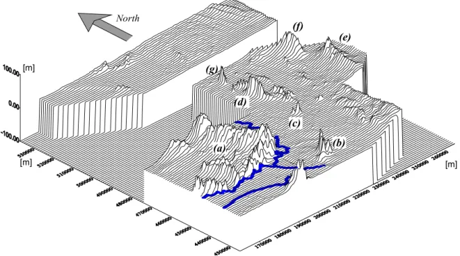
Figure 2 gives a three-dimensional view of the surface elevation with respect to Dutch datum level (NAP). The elevation varies between – 4 and 103 metres (NAP). Notice the presence of several ice-pushed ridges, where the elevation is higher than the direct surroundings.

Figure 2. Three-dimensional view of the surface elevation. (a) Veluwe

(b) Montferland (c) Lochemerberg

(d) Holterberg (Nijverdal) (e) Lonnekerberg (Oldenzaal) (f) Ootmarsum (g) Lemelerberg (g) (f) (e) (d) (c) (b) (a) [m] [m] [m] North

3.2 Surface waters

The Rhine River, some of its branches (IJssel and Waal) and several smaller rivers are running through the southern part of the area. In the east several minor watercourses, such as the Slingebeek, Baakse Beek, Berkel, etc. follow the general descending inclination of the surface in eastwestern direction. All these streams finally discharge into the IJssel. This means that in fact the IJssel takes care of the drainage for most of the eastern section of the area. The part of Twente located north of the Schipbeek/Twente Canal discharges via De Regge and Dinkel into the Overijsselse Vecht along the northern edge of the area (see Figure 3).

The central part of the Veluwe/Achterhoek area consists of the IJssel Valley, where the IJssel River runs northward. The IJssel finally discharges in the lake IJsselmeer (not shown in the figure).

Figure 3. Surface-waters in the study area.

160000 170000 180000 190000 200000 210000 220000 230000 240000 250000 260000 270000 430000 440000 450000 460000 470000 480000 490000 500000 510000 520000 530000 IJss el Slingebeek Oud e IJs_sel

Baakse _{Beek Berkel}

Twente Kanaal IJssel Schipbeek Din kel Re_gg e O. Vecht Schip_beek O. Kana_al

Kanaal Almelo-Noorh.

Neder Rijn Linge Waal Grift [m] [m] Veluwe Twente Achterhoek Hoogeveen

3.3 Aquifer system

The thickness of the Pleistocene complex that comprises the aquifer system varies considerably. At the southeastern side the thickness is between 10 and 30 metres. In the northwestern direction the thickness increases to 300 metres and more. This is due to the rapid decline of the low permeable Breda Formation, which is considered to be the base of the geohydrological system. Figure 4 presents a contourmap of the base elevation. Detailed geological descriptions of the area can be found in Grootjans (1984) and Vermeulen et al. (1996), as well as in the NAGROM/TNO report (Anonymous, 1993).

Figure 4. Contours of the base of the aquifer system.

170000 180000 190000 200000 210000 220000 230000 240000 250000 260000 430000 440000 450000 460000 470000 480000 490000 500000 510000 520000 530000

Depth in metres NAP (Dutch datum level)

[m]

Figures 5 and 6 show the presence and thickness of the first (Eemian-clay) and second aquitard (Drenthe/Tegelen-clay) as modelled in LGM.

Figure 5. Presence and thickness of the first aquitard (Eem-clay).

160000 170000 180000 190000 200000 210000 220000 230000 240000 250000 260000 270000 430000 440000 450000 460000 470000 480000 490000 500000 510000 520000 530000 0 1 2 3 4 5 6 7 8 9 10 11

Thickness first aquitard in metres

[m]

Figure 6. Presence and thickness of second aquitard (Drenthe-clay). 160000 170000 180000 190000 200000 210000 220000 230000 240000 250000 260000 270000 430000 440000 450000 460000 470000 480000 490000 500000 510000 520000 530000

Thickness second aquitard in metres

0 3 6 10 15 20 25 30 35 40 45 50 55 60 65 70 75 80 [m] [m]

3.4 Groundwater heads and velocities

As mentioned in Chapter 2, the groundwater heads and velocities have been determined in a previous study (Kovar et al., 1998) by means of the National Groundwater Model (LGM, see also Chapter 5). The groundwater flow model is applied as a stationary model. Hence, the heads and velocities presented here are considered to be representative for an average situation over a longer period of time (several years). Figure 7 shows the distribution of the groundwater head in the upper aquifer.

Figure 7. Groundwater heads in upper aquifer as determined by LGM in metres with respect to datum level (NAP).

-1 4 9 14 19 24 29 34 39 44 49 54 59

Groundwater head

m

This picture reflects the surface relief in a less pronounced manner. It shows a general decrease from the southeastern edge towards the IJssel valley in the central part. The higher heads under the ice-pushed Veluwe-hills in the southwest are clearly visible. Other ice-pushed ridges (Montferland, Nijverdal, Ootmarsum and Oldenzaal) can also be observed and

associated with higher heads.

Figures 8 and 9 present the groundwater velocities at the depth of 0.1 m below the phreatic surface. The vertical component is displayed as a contourplot (Figure 8). Blue and blue-grey shades are indicative for an upward velocity (seepage), while yellow to red shades denote downward flow (i.e. infiltration). As it appears, the location of the ice-pushed ridges determines the pattern of infiltration for the greater part. Especially the Lemelerberg and Nijverdal emerge as dominant infiltration areas.

The horizontal velocity has been displayed in Figure 9 as a vector plot. The arrows indicate the direction of the flow, while the magnitude of the arrow indicates the magnitude of the velocity.

Figure 8. Vertical groundwater velocity at 0.1 m below phreatic surface. 160000 170000 180000 190000 200000 210000 220000 230000 240000 250000 260000 270000 430000 440000 450000 460000 470000 480000 490000 500000 510000 520000 530000 -0.020 -0.016 -0.012 -0.008 -0.004 0.000 0.005 0.010 0.020 0.200 Infiltration (m/day) [m] [m] Seepage (m/day)

Figure 9. Direction and magnitude of horizontal groundwater velocities at 0.1 m below the phreatic surface. 160000 170000 180000 190000 200000 210000 220000 230000 240000 250000 260000 270000 430000 440000 450000 460000 470000 480000 490000 500000 510000 520000 530000 [m] [m] 0.5 m/day 0.25 m/day

4

Groundwater abstraction

4.1 Rates of discharge

In the study area a large number of industrial wells and private groundwater abstractions are present as well as a number of pumping stations abstracting water for public drinking water supply. The total groundwater abstraction for public water supply has increased substantially during the period 1960-’80. Since then, the level of abstraction more or less remained

constant, while after 1990 a slightly decreasing trend can be observed. Examples are shown in the Figures 10 and 11. These graphs give the total amount of water (in million m3 year-1) abstracted for public water supply by the pumping stations in 2 of the 4 model areas. Industrial and private groundwater abstractions are not included in the graphs, but they are taken into account in the model. In both areas (Achterhoek and Twente) the industrial and private abstractions are approximately 50% of the total abstracted volume.

Figure 10. Yearly abstracted volume of groundwater by pumping stations in model area Achterhoek.

Groundwater Abstraction Achterhoek

0.0 10.0 20.0 30.0 40.0 50.0 1950 1953 1956 1959 1962 1965 1968 1971 1974 1977 1980 1983 1986 1989 1992 1995 1998 year Volume [ M m 3 /y ]

Figure 11. Yearly abstracted volume of groundwater by pumping stations in model area Twente.

4.2 Locations

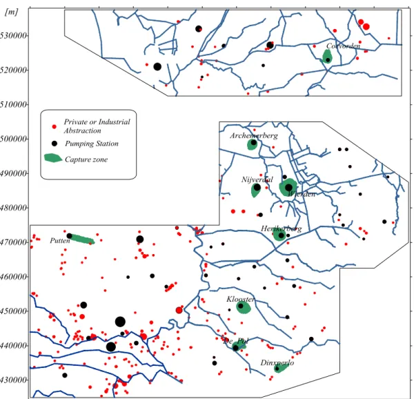
The locations of all groundwater abstractions are displayed in Figure 12. Private and

industrial abstraction wells (with a discharge larger than 50000 m3 year -1) are indicated as red circles, while the public water supply pumping stations are shown as black circles. The sizes of these circles are proportional to the amount of abstraction. In the present report attention is focused on 9 public water supply pumping stations, which were randomly selected throughout the central and eastern part of the Netherlands. In this part of the country the occurrence of nitrate in groundwater is a topical subject. For the selected pumping stations also the capture zone is given in green (Figure 12).

Groundwater Abstraction Twente

0.0 10.0 20.0 30.0 40.0 50.0 1950 1953 1956 1959 1962 1965 1968 1971 1974 1977 1980 1983 1986 1989 1992 1995 1998 Year Volume [ M m 3 /y ]

Figure 12. Location of the groundwater abstractions and the capture zones of selected pumping stations. 160000 170000 180000 190000 200000 210000 220000 230000 240000 250000 260000 270000 430000 440000 450000 460000 470000 480000 490000 500000 510000 520000 530000 Klooster De_Pol Dinxperlo Archemerberg Nijverdal Herikerberg Wierden Putten Coevorden [m] [m] Pumping Station Private or Industrial Abstraction Capture zone

5 Data and models

5.1 Nitrate measurements

Parameter estimation or calibration is the process of fitting measured data with data generated by the model that includes the unknown parameter(s). The set of nitrate measurements used in this report may be divided into two categories. The first category consists of data from

monitoring wells (Monitor Well Data). These data originate from the National Groundwater Monitoring Network, which has been installed during 1979-1984 (Snelting et al., 1990). Groundwater samples are collected at least annually at various filter depths (up to 30 metres below surface). The volume of the water samples is relatively small in comparison to the spatial resolution of the groundwater transport model. For, instance, a calculated

concentration represents a volume 125 × 125 ×10 m3, while the measurements are based on a volume of several litres. Therefore, in practice, the measurements may be regarded as point measurements. From detailed local studies it is known that nitrate levels fluctuate during the year and vary considerably in space as well. The data used in this study are representative for four moments in time, respectively the years 1982, 1990, 1995 and 2000. In order to obtain the data in the right format, some pre-processing and averaging has been applied. For a certain moment t the measurements are averaged over an interval starting at t - 500 days until t + 500 days. In a few cases data from local monitoring networks have been added to the data set. The second category of data (Breakthrough Data) consists of nitrate contents measured at the pumping stations. The main difference with the monitoring data is that breakthrough data refer to a mixture of waters that have infiltrated at different locations and at different times. Therefore, this is a mixture of waters with different ages and origins. Nitrate measurements at the pumping stations should preferably be taken from the water before the purification process. For most pumping stations nitrate contents have been collected since 1992 in the so-called REWAB programme (in Dutch: REgistratie opgaven van WAterleidingBedrijven). These measurements refer to the untreated water as well as the water after purification. A longer series of data is available from the LMD measuring programme (in Dutch: Landelijk Meetnet Drinkwaterkwaliteit), which refers to the nitrates of the water after the purification. In the purification process no specific nitrate decontamination is applied and in a number of cases the measurements in the treated and untreated water hardly differ. However, this does not hold for all pumping stations.

5.2 Leachate model

At present STONE is being used as the standard tool in national scale nutrient leaching studies. STONE (Beusen et al., 2000; Overbeek et al., 2001a) calculates the flux of several

nutrients from the root zone into the groundwater system on a temporal basis of decades (10 days). The spatial differentiation of the model results is obtained by applying the model for a large number of unique combinations of soil type, land use and hydrological features. For the present study area nitrate leaching rates have been calculated by STONE within the

framework of the fifth National Environmental Outlook. These are described in more detail by Overbeek et al. (2001b). The temporal resolution of 1 decade of days of the STONE data is too detailed for the solute transport model. Therefore, the data have been transformed into 15-year averages for the interval from 1950-2000.

5.3 Groundwater model

As mentioned before, Kovar et al. (1998) calculated the groundwater heads and velocities in the area with the groundwater flow model National Groundwater Model LGM (Pastoors, 1992; Kovar et al., 1992). LGM is based on finite elements and describes the groundwater flow in a multi-aquifer system separated by one or more aquitards. Within each aquifer the head distribution is treated two-dimensionally in horizontal direction, while through the aquitards purely vertical flow is assumed. In terms of groundwater velocities the model is quasi-three-dimensional. The horizontal flow components are derived from Darcy’s low, while the vertical flow is obtained by an approximate procedure, known in the literature as Strack’s interpretation of Dupuit-Forchheimer (Strack, 1984). In short, the approximation may be formulated as follows: within the aquifers vertical conductivity is assumed infinitely large, while in the aquitards the horizontal conductivity is assumed to be zero.

At the top of the upper aquifer, interaction occurs between the groundwater and the drainage system of ditches and drainage tiles. This zone is referred to as the top-system. In principle natural recharge infiltrates at the phreatic surface. This vertical groundwater flux is denoted by qre. A portion of this recharge may leave the underground after a relatively short stay (e.g.

several days) and discharge into the drainage system. The latter portion is referred to as the top system discharge, denoted by qts. The top system discharge plays a role in the

determination of the nitrate flux that reaches the groundwater.

The top system discharge is taken into account in the groundwater model via the following expression: 0 ts h q c j -= (1)

where the coefficient c is the so-called drainage resistance (days), h is the zero drainage₀

level (drainage base) and j(x,y) is the groundwater head as calculated by LGM. The amount of water infiltrating into the aquifer system, qas, is qre - qts or:

0 as re h q q c j -= - (2)

Note that qre , h0 and c are all given input parameters, while both j(x,y) and also qas, need to

be calculated by the model. When j is greater than h0 , the aquifer system discharges water

into the drainage system. Irrigation occurs when j is less than h0 , i.e. water infiltrates from

the ditches and drains into the aquifer. Both h0 and c may vary in space, so qts also is a

function of the horizontal co-ordinates x and y. The parameters c, h0 and qre are all given as

model input.

The drainage or irrigation that take place in the top-system is not only relevant for the mass balance of water, but also for the net amount of nitrate that finally enters the aquifer system. Together with the discharge qts an amount of nitrate is removed via the drainage system. This

nitrate term must be taken into account. In case of infiltration/irrigation an additional amount of water enters the aquifer. The nitrate content of this term is unknown. In this study it is assumed to be zero.

Figure 13. Scheme of the Top-system.

In principle, LGM can be applied for non-stationary flow situations, but in the present and previous studies steady conditions have been assumed. The recharge data represent recharge from the year 1988, which is considered to be a rather ‘wet’ year. Model parameters such as aquifer transmissivities and aquitard resistance have been calibrated on measured head data (Leijnse and Pastoors, 1996).

5.4 Solute transport model

The next modelling step concerns the nitrate transport. The LGM-package includes the solute transport module LGMCAD (Uffink, 1996, 1999). LGMCAD uses the particle tracking technique, which means that during the calculating process particles are introduced in the aquifer. The particles are characterised by several time dependent attributes, such as x, y and z co-ordinates and a (solute) mass m, here representing a certain amount of dissolved nitrate. The model calculates the displacement and mass changes for each particle separately. The particle displacement consists of a deterministic component that describes advective transport and a stochastic component that accounts for the dispersive transport. More information on this modelling technique and its application in LGMCAD is found in Uffink (1990) and Kinzelbach and Uffink (1991).

The main input data for the transport model are the (3D) groundwater velocity distribution for the aquifer and the nitrate fluxes at the upper boundary. The groundwater velocity distribution is provided the groundwater flow module (LGMFLOW). Nitrate fluxes at the phreatic surface have been generated with the leaching model STONE. Observations show that in the vertical direction steep nitrate concentration gradients occur. To retain such gradients in the

simulation, special attention is required to the simulation of vertical mixing processes. Numerical dispersion should be avoided by all means, since it would destroy all vertical resolution. The random walk particle technique is an effective procedure in this respect, since numerical dispersion is absent. Small vertical dispersivity values are used.

As stated earlier, nitrate transport in the aquifer can only be simulated when information is available on the amount of nitrate entering the aquifer from the unsaturated zone. This information forms the upper boundary condition in terms of solute fluxes. The leaching data generated by STONE need to be pre-processed before an adequate upper boundary condition can be set up. This is due to the rather complicated situation at the upper boundary (top-system) and the fact that STONE and LGM are based on different modelling concepts for the top-system.

Schematically the situation is as follows. At the bottom of the unsaturated zone a hypothetical surface is considered, through which a downward groundwater flux qre(x, y) occurs. Since the

groundwater flow model is stationary, this term does not depend on time. When the nitrate concentration is denoted by cN(x, y, t), the nitrate flux Fre, through this surface is the product cN × qre. Note that contrary to the water flux, the nitrate flux does depend on time since the

concentrations depend on time. In the absence of the drainage system the product cN × qre

provides the upper boundary solute flux for the transport model. However, due to the drainage system, the actual water flux into the system, may be reduced to qas , as given by eq. (2), and

and solute transport model, since cN is produced by STONE, while qas is determined by

LGM. However, in the leaching model the situation is more complicated since it describes not only the unsaturated zone, but also part of the saturated zone and thus part of the drainage system. Further, instead of the (stationary) hypothetical surface considered in the groundwater we have a fluctuating phreatic surface. Since the model concepts that are used are essentially different, it is not directly clear what depth must be chosen to couple the two models. In the present study we use the STONE data at the so-called GHG-level (mean highest groundwater head). This level is a standard depth for the STONE output. Overestimated nitrate flux may be expected when these data are used, since nitrate concentrations demonstrate a rapid decrease with depth between GHG-level and GLG-level (mean lowest groundwater head). Even directly below GLG-level a rapid decrease of nitrates occurs. Overbeek et al. (2001b) have reported a nitrate reduction with 20-25% in the first 0,5 meter below GLG. The

overestimation in the nitrate flux may be compensated when a reduction factor or zero-order denitrification concept is included in the denitrification module. This is described in more detail in Chapter 6.

6 Denitrification

6.1 General

Denitrification in the unsaturated zone and the upper zone of the aquifer is quite well documented (Mariotti, 1986; Hiscock et al., 1991; Korom, 1992). Also a substantial

denitrification is known to occur in the deeper zones of the aquifers, although the latter has been less frequently reported (e.g. Lawrence and Foster, 1986). Nitrates are generally found to be relatively stable in aerobic groundwater. However, as oxygen is consumed, nitrate may become the source of energy for microbial life. Subsequently, the nitrate content is reduced. On many places where, based on conservative transport, nitrate is expected, it appears to be absent or the concentration has decreased to a level that can not be explained by dilution or dispersion only. Although at present the theoretical mechanism of denitrification is rather well understood, at field situations there is little information on where, when and at what rate denitrification can be expected.

Denitrification refers to the reduction of nitrate first to nitrite and finally into N2. The process

takes place through mediation of bacteria. Generally, the bacteria are assumed to be present always and everywhere in the aquifer. Normally the bacteria use oxygen for their energy supply, but in anaerobic conditions they switch to an anaerobic metabolism using nitrates. Besides anaerobic conditions the presence of an electron donor is required, which can be either organic or inorganic. Furthermore, the bacterial activity is dependent on temperature and pH. In practice, the presence of the electron donor appears to be the limiting factor for the occurrence of denitrification. Usually the electron source consists of organic material.

Inorganic denitrification (e.g. by pyrite) also occurs, but is less common (Hiscock et al., 1991).

Indicative for the occurrence of denitrification is, besides the low oxygen content, a high sulphate content in case of pyrite-oxidation (Kölle et al., 1985), while bi-carbonates contents are increased in case of organic denitrification (Trudell et al., 1986). In the case of reduction of pyrite usually sharp nitrate fronts are found. Therefore, it may be concluded that

denitrification by pyrite occurs almost instantaneously. Denitrification based on reduction of organic material is a much slower process. According to Van Beek et al. (1994) this is due to the slow rate at which organic material becomes available to the bacteria. The greater organic molecules cannot be used directly by the bacteria and first must be transformed into smaller ones. According to Van Beek this so-called decomposition process may be described as a first-order decay process. In that case, it may be modelled by an exponential function of the travel time exp(-lt). Strictly speaking the decay rate l rather reflects the rate of

time, T , which expresses the time needed to reduce the initial concentration by a factor ½._½

Half-life time and decay rate are related by ½

ln 2 0.7

T

l l

= ; (3)

Especially in artificial denitrification projects the biodegradation process has been studied intensively. Artificial denitrification is a technique where on purpose nitrates are added to the groundwater in order to stimulate the bacteria in their degradation process. In those cases the final objective is to reduce the amount of organic contaminants. Often, in these studies the kinetics are described by the so-called Monod equation, which is of the following form:

dc c a

dt = - K c+ (4)

where K and a are constants. Mathematically, this non-linear equation is difficult to model, but for low concentrations (c= K) it may be approximated by a first-order (exponential) equation (Bekins et al., 1998):

dc a c

dt = -K (5)

For higher concentrations, however, the first order approximation leads to an overestimated nitrate reduction.

6.2 Implementation

A first order decay process is easy to implement in a solute transport code that applies particle tracking. Uffink and Römkens (2001) have obtained experience with the exponential

denitrification model. It appeared that results obtained with a single decay parameter (no zones) were not satisfactory. Therefore a spatial (zonal) distribution of the parameter was proposed. At first a constant ‘background’ value is assigned everywhere in the aquifer system. This value is changed in a zone of 5 metre directly above and beneath the major clay-layers (aquitards) and in the direct vicinity of local streams and rivers. The reasoning behind this approach is that in these zones more organic material is present and therefore a higher denitrification capacity may be expected. For instance Meinardi (1999) has observed in a study area in the Achterhoek (Hupsel) that denitrification occurs when the deep groundwater is in contact with the clay inclusions at the base of the aquifer. The decay-parameters found by Uffink and Römkens, expressed as half-life times, are ranging from 200 to 2000 days. In the present transport model, besides a first order decay, an additional type of denitrification has been implemented. Directly after the groundwater (and nitrate) has entered the aquifer an

instantaneous nitrate reduction is considered to occur. This is referred to as the zero-order nitrate reduction. As the groundwater continues its path into the deeper zones, nitrates further decrease according to the exponential first-order equation.

An example of nitrate reduction in time is given in Figure 14. The graph presents the mass change from the moment a particle infiltrates into the aquifer. The moment of infiltration is taken as t=0 , while the initial mass is M . Further, we assume that the aquifer consists of₀

two zones A en B with decay-rates l and _A l , respectively. During simulation, the actualB

moment of infiltration and particle mass is determined from the leaching data. After time t the particle has travelled through zone A during an interval tA, and through zone B during tB,

where t = tA + tB. Then, we may write for the particle mass at time t:

0

( ) exp( _{A A B B})

M t =M e -l t -l t (6)

Figure 14. Changes of particle mass, during transport.

The reduction coefficient e (e < 1) represents a rapid nitrate reduction right before the particle enters the saturated groundwater. To stay in line with the first-order notation we may write this as: 0 0 exp( ) e = -l t (7) 0 0

1

M

_é

_-

e

_ù

ë

û

M

0

where l0 is a (high) denitrification rate that is supposed to occur in a very short time t0. The

concept of a zero order denitrification implies that the product t0l₀ remains constant when

¥ ®

® 0

0 0,l

t . So, with Λ0 =t₀l₀ this leads to:

0 0

( ) exp( _{A A B B})

M t =M - -Λ l t -l t (8)

The concept of exponential decay has also been applied by Wendland (1992) to describe denitrification in similar aquifer types in Germany. However, the decay parameter l should not be associated too closely with the actual denitrification processes. According to Van Beek et al. (1984) it also reflects the decomposition process of the organic material. This also means that its value may not be derived directly from soil-parameters. So far, values can best be guessed or, when data from measurements are available, determined by calibration

techniques, as is done in the present report. Obermann (1982) has applied a reduction factor, similar to the zero order term proposed here. For the lower Rhine region in Germany factors are reported of 0.16, 0.63 and 0.70 (Haag and Kaupenjohann, 2001).

For the spatial distribution of the exponential decay rates a zonal approach is applied, which means that in the model area two zones are defined. One zone covers a default or background zone, where the decay rate is considered to be low. Then, in the aquifer system a second zone is identified, where the decay rate is expected to be higher, e.g. because it may be expected that in this zone more organic material is present. For the present study the high decay rate is applied in a layer of 5-metre thickness above and underneath the claylayer (first aquitard) and in all gridcells adjacent to rivers and minor courses of surface water. The same distribution scheme has been used in Uffink and Römkens (2001) as well as in Uffink and Mülschlegel (2002). The location of the surface water and rivers has been displayed in section 3.2, while the occurrence of the claylayers has been presented in section 3.3.

Finally, a spatial pattern emerges that in vertical direction is composed of three layers. Within each layer a regular grid with 500 x 500 m cells is defined. In each gridcell the decay rate is either equal to l or _A l . The allocation of the decay rate depends on whether a claylayer isB

present or not, or whether the cell is underneath a river or stream. The elevation and thickness of the middle zonal layer is directly related to the Drenthe-clay-layer. In case clay is present, the layer is defined between 5 metres above the top of the clay until 5 metres underneath the bottom. At those location where the clay is absent the actual elevation of the layer is not relevant since here no distinction between the layers exists. The upper zonal layer extends vertically from the surface to the top of the middle layer, while the lower zonal layer runs from the bottom of the middle layer to the base of the aquifer system.

Figure 15 shows schematically the vertical set-put of the layers. The distribution of the decay rate in the upper and middle zonal layer is given in Figure 16 and 17. The horizontal

distribution in the lower zonal layer is identical to the upper layer.

Figure 15. Schematic vertical cross-section with zonal layers. Layer 1

Layer 2 Layer 3

decay rate overwritten decay rate overwritten

- under valleys of brooks/rivers - under and above claylayer(s)

Figure 16. Zonation for calibration of decay rate in layer 1 and 3. 160000 170000 180000 190000 200000 210000 220000 230000 240000 250000 260000 270000 430000 440000 450000 460000 470000 480000 490000 500000 510000 520000 530000 layer 1 and 3 [m] [m]

Figure 17. Zonation for calibration of decay rate in layer 2. 160000 170000 180000 190000 200000 210000 220000 230000 240000 250000 260000 270000 430000 440000 450000 460000 470000 480000 490000 500000 510000 520000 530000 [m] [m]

7 Calibration

7.1 Parameters

The parameters to be estimated during the calibration procedure are the denitrification constants L0 , λA and λB , as given in equation (6). In the simulation programme, however,

these parameters are given in an alternative notation [see eq. (3) and (5)]: - ε : zero order reduction term [-]

- ½

A

T first order decay-rate, zone A [T]: - ½

B

T first order decay-rate, zone B [T]

In this pilot study nine pumping stations have been selected (sect 4.2, Figure 12). For each selected pumping station a separate calibration exercise is performed using nitrate

measurements from the monitoring wells located in a 20´ 20 km2 area around the pumping-station and the breakthrough data from the pumping well itself. Hence, for each pumping station a separate set of the parameters given above is obtained. These parameter values are representative only for the area around the pumping station. Note that the monitoring wells do not exclusively lie inside the capture zone and, consequently, the representative area is not restricted to the capture zone.

7.2 Log transform of concentrations

During a calibration procedure the unknown model parameters are varied, while for each set of values the match between measured data and model outcomes is examined. The parameters that yield the ‘best’ match between model results and measurements are considered as the best estimates. Calibration has been applied successfully to estimate the aquifer transmissivities and hydraulic resistances of aquitards for the groundwater flow model (LGM) for the Netherlands (Leijnse and Pastoors, 1996). Leijnse and Pastoors used observed groundwater heads for their calibration. For the present problem observed groundwater heads are useless, since the unknown denitrification parameters do not affect groundwater heads. For the present calibration exercise the most adequate data consist of measurements of groundwater nitrate concentrations. The user still is still free to choose in what way measured and observed data are expressed, e.g. linear or logarithmic.

The magnitude of the measured nitrated values varies within a wide range. Therefore, a calibration based on the ratios between predicted and measured concentration (or differences of the logarithms of the concentrations) makes more sense than using the concentration

differences directly. The effect of the log-transform is best illustrated by the simple example. Consider two monitoring wells A and B. In well A measured and calculated concentrations are, respectively 102 and 103, while in well B measured and calculated concentrations are 2 and 3. When the difference between measurements and model values to determine the goodness of the match, it appears that the match is equally well for both wells. However, when we want to expressed that at well A the calculated value is less than 1% off, while at well B the model outcome is 50% larger than the measured value, we need to consider

logarithms of measured and calculated values. In general, if one is interested in relative errors rather than absolute errors it is more natural to consider the logarithm of the model outcomes and measurements. In this study we consider the log-transformed concentrations, since we are dealing with a wide range of concentration values and a relative error seems more relevant than an absolute error:

ln m m i i Y = c (9) ln c c i i Y = c (10)

Superscript m (measured) and c are used for observations and calculated values, respectively. The index i denotes an individual measurement, while cic represents the calculated

concentration at the place and time of the ith measurement. The difference between measured value and model outcome at location i is known as the residual. During the calibration procedure an objective function E is optimised, which is defined as the sum of the weighted (squared) residuals:

(

)

_{Y Y}

å

where γi denotes a weight factor and N is the total number of observations. Weights may be

used to express the importance of an observation with respect to the rest of the measurements. Weights may be used in various ways to control and manipulate the calibration process. For instance if one wants to exclude a particular observation from it calibration process, either temporarily or permanently, this can be achieved by a weight factor of zero. The objective function E may be optimised by techniques such as Gauss-Marquardt-Levenberg method. For further details see e.g. Cooley (1983) or Hill (1992).

7.3 Software

Calibration is performed with the programme PEST (Parameter Estimation). PEST is a model independent parameter optimisation programme developed by Doherty of Watermark

field of groundwater flow. It uses a non-linear optimisation technique, based on the Gauss-Marquardt-Levenberg method. Various versions of PEST exist, both commercial and free (but limited) versions. In this study a freeware version has been used that runs on a DOS platform. (Anonymous, 1994). The groundwater nitrate transport simulations, however, are running on UNIX machines. Several tools and scripts have been written to handle command switches between the PC and UNIX machines. The advantage of the use of PEST is that the simulation programme itself does not have to be modified to perform the calibration. A disadvantage is that the programme PEST is used as a ‘black box’. For instance, intermediate results of the calibration process, such as the sensitivity matrix, are not given as output and remain inaccessible. In the present study e.g., the sensitivities would have provided useful information to obtain a stable calibration procedure (see 7.4).

7.4 Procedure

Preliminary runs showed that calibration based on breakthrough data alone did not lead to a unique set of decay-parameters. When only the breakthrough data are used a so-called ill-posed problem arises. The system becomes better defined, when –in addition to the

breakthrough data– measurements from the monitoring wells are included. Problems due to the ‘ill-posed-ness’ may be circumvented by using a step-wise calibration procedure. At each step only a single parameter is free to be varied, while the other are kept constant. Only observations are used with a high sensitivity to the free parameter. For this approach

information on the sensitivity matrix would be helpful. As mentioned above, PEST does not provide this information. As an alternative, observations have been selected based on a more intuitive argument. This has led to the following step-wise procedure.

– Step 1. First, a calibration run is performed without the breakthrough data using only monitor well measurements from the shallow filters. Switching off the breakthrough data can be realised easily by setting the weights equal to zero. The purpose of the first run is to calibrate the zero-order decay term. The nitrate levels measured at shallow depth are the most affected by the zero-order parameter, since the residence times are still relatively short and the first-order decay has not been active very long. In this step, only the zero-order and one of the first-zero-order (the fast one) are allowed to vary. The slow exponential decay is set at a constant value (_T½A _{is 5000 days).}

– Step 2. Accordingly, the zero-order reduction parameter is frozen at the level found in step 1. Both shallow and deep monitoring data are included, while we calibrate only the two exponential decay parameters. The results of this run are given in the appendix. – Step 3. All observations are included. In the final step all parameters are allowed to vary,

but the ratio between _T½A_and

½

B

8 Results

8.1 Calibration results

The transport model LGMCAD combined with PEST has been applied for a 20´20 km2 area around each selected pumping station. The Figures 18 to 26 give the location of the

monitoring wells and capture zone of the pumping station projected on a map of the zonal distribution of the decay parameter. The figures at the left-hand side give the zonal

distribution of the layers 1 and 3 (upper and bottom layer), while at the right-hand side figures show the zonation in layer 2 (middle layer). Note that the middle layer encloses the clay-layer (aquitard). The zonal distribution in this layer only differs from the one in the top layer at the places where the clay layer indeed exists. For each pumping station a set of parameter values has been obtained. The final results are given in Table 2. For the pumping station Putten the final denitrification values could not be obtained. In principle it may be concluded that at

Putten no denitrification occurs. The model residuals for the pumping well data remain

positive, even for extremely high values of the half-life time (very slow denitrification) and a zero-order reduction factor equal to 1.0. In terms of nitrates a positive residual says that model result shows less nitrate than is observed in the real system. In fact, when the zero-order reduction factor is not bounded by an upper limit of 1.0, a value of 1.4 is obtained. This may be an indication that nitrate fluxes are underestimated, while it also demonstrates that the instantaneous (zero-order) reduction does not occur here. At pumping station Klooster the values for the two zones appear to be essentially the same. For an explanation refer to Figure 21. In this figure it is seen that most of the shallow monitoring filters and the entire capture zone of the pumping wells are located in one and the same zone (zone A). Only a few monitoring wells are located in zone B, but very near to the border between the two zones. Note that the exact borders are drawn somewhat arbitrarily. Therefore, for this particular part of zone B a really faster decay parameter is not likely. It may be concluded that this area in fact belongs to zone A. At the pumping station Coevorden the breakthrough data for nitrate are extremely low. Almost all nitrate appears to be removed by denitrification (see also sect. 8.4). The calibration procedure results in a zero order reduction rate of 5%. However, it is doubtful whether this is a realistic, physical value. A final set of half-life times could not be obtained here.

Table 2. Final Calibration Results. Slow-zone (_T½A₎ [days] Fast-zone (_T½B₎ [days] Zero-order (e ) De Pol 4468 3017 0.37 Archemerberg 4063 2804 0.71 Herikerberg 1801 421 0.59 Klooster 2612 2487 0.17 Dinxperlo 2492 843 0.22 Nijverdal 2207 64 0.41 Wierden 5075 634 0.29 Putten ( >20000) ( >20000) (>1.00 ) Coevorden < 0.05

Figure 18. Location of monitoring wells and capture zone for pumping station De Pol with zonation of denitrification parameter as background.

215000 220000 225000 230000 430000 435000 440000 445000 450000 slow fast Middle Layer 215000 220000 225000 230000 430000 435000 440000 445000 450000 Monitoring Well

Top and Bottom Layer

Capture Zone PS

Figure 19. Location of monitoring wells and capture zone for pumping station Archemerberg with zonation of denitrification parameter as background.

Figure 20. Location of monitoring wells and capture zone for pumping station Herikerberg with zonation of denitrification parameter as background.

slow fast

Middle Layer

Monitoring Well Capture Zone PS

225000 230000 235000 240000 245000 465000 470000 475000 480000 485000 225000 230000 235000 240000 245000 465000 470000 475000 480000 485000

Top and Bottom Layer

slow fast

Middle Layer

Monitoring Well Capture Zone PS

220000 225000 230000 235000 490000 495000 500000 505000 220000 230000 490000 495000 500000 505000

Figure 21. Location of monitoring wells and capture zone for pumping station Klooster with zonation of denitrification parameter.

Figure 22. Location of monitoring wells and capture zone for pumping station Dinxperlo with zonation of denitrification parameter.

slow fast

Middle Layer

Monitoring Well Capture Zone PS

215000 220000 225000 230000 440000 445000 450000 455000 460000 215000 220000 225000 230000 440000 445000 450000 455000 460000

Top and Bottom Layer

slow fast

Middle Layer

Monitoring Well Capture Zone PS

230000 235000 240000 245000 425000 430000 435000 440000 445000 230000 235000 240000 245000 425000 430000 435000 440000 445000

Figure 23. Location of monitoring wells and capture zone for pumping station Nijverdal with zonation of denitrification parameter.

Figure 24. Location of monitoring wells and capture zone for pumping station Wierden with zonation of denitrification parameter.

slow fast

Middle Layer

Monitoring Well Capture Zone PS

220000 225000 230000 235000 475000 480000 485000 490000 495000 220000 225000 230000 235000 475000 480000 485000 490000 495000

Top and Bottom Layer

slow fast

Middle Layer

Monitoring Well Capture Zone PS

230000 235000 240000 245000 475000 480000 485000 490000 495000 230000 235000 240000 245000 475000 480000 485000 490000 495000

Figure 25. Location of monitoring wells and capture zone for pumping station Putten with zonation of denitrification parameter.

Figure 26. Location of monitoring wells and capture zone for pumping station Coevorden with zonation of denitrification parameter.

slow fast

Middle Layer

Monitoring Well Capture Zone PS

165000 175000 185000 460000 470000 [m] 165000 175000 185000 460000 470000 [m]

Top and Bottom Layer

slow fast

Middle Layer

Monitoring Well Capture Zone PS

240000 250000 520000 530000 240000 250000 520000 530000