Risk-based standards for PCBs in soil : Proposals for environmental risk limits and maximum values

Hele tekst

(1)Risk-based standards for PCBs in soil Proposals for environmental risk limits and maximum values RIVM report 2014-0119 E.M.J. Verbruggen | E. Brand.

(2)

(3) Risk-based standards for PCBs in soil Proposals for environmental risk limits and maximum values. RIVM Report 2014-0119.

(4) RIVM report 2014-0119. Colophon. © RIVM 2014 Parts of this publication may be reproduced, provided acknowledgement is given to the 'National Institute for Public Health and the Environment', along with the title and year of publication.. Eric M.J. Verbruggen (Senior Risk Assessor), RIVM Ellen Brand (Researcher), RIVM. Contact: Eric Verbruggen Centre for safety of substances and products eric.verbruggen@rivm.nl. This investigation has been performed by order and for the account of the Ministry of Infrastructure and the Environment, department of sustainability, within the framework of soil quality.. This is a publication of: National Institute for Public Health and the Environment P.O. Box 1│3720 BA Bilthoven The Netherlands www.rivm.nl/en Page 2 of 64.

(5) RIVM report 2014-0119. Abstract. Risk-based standards for PCBs in soil Proposals for environmental risk limits and maximum values The RIVM proposes new science-based quality standards for PCB contaminants (polychlorinated biphenyls) in the soil. This is necessary to assess the possibilities for the reuse of excavated soils. The quality of the soil determines the type of land use for which the soil can be reused. If the quality is high enough, this can be the land use ‘residential with garden’, if not it can be reused for the land use 'industrial'. For the reusing of soil it is determined which contaminants are in the soil by use of a standard list. In 2008, PCBs were added to this list of substances. The quality of the soil is determined based on the proposed quality standards (socalled maximum values). To date, however, there have been no scientifically based maximum values for PCBs. The proposed science-based quality standards for PCBs in soil are based on the exposure of mustelids to PCBs. It appears that mustelids are designated as the family of animals that are most sensitive to PCBs. Up to now, the risk limits of PCBs in the soil were based only on the direct toxicity of these substances for humans and ecosystems. However, the accumulation of PCBs in the food chain is a greater risk than direct toxicity. If accumulation in the food chain is not included in risk assessment, the risk is underestimated.. Keywords: Polychlorinated biphenyls (PCBs), maximum values, risk assessment, ecosystems, secondary poisoning, human. Page 3 of 64.

(6) RIVM report 2014-0119. Page 4 of 64.

(7) RIVM report 2014-0119. Publiekssamenvatting. Risico onderbouwde normen voor PCB’s in de bodem Voorstellen voor risicogrenswaarden en maximale waarden Het RIVM doet een voorstel voor nieuwe wetenschappelijk onderbouwde normen voor PCB-verontreinigingen (polychloorbifenylen) in de bodem. Dit is nodig om te beoordelen voor welke doeleinden afgegraven grond kan worden hergebruikt. De kwaliteit van de grond bepaalt óf dat kan en voor welke bestemming het mag worden hergebruikt: bij voldoende kwaliteit voor ‘wonen’, anders voor ‘industrie’. Voor de beoordeling van hergebruik van grond wordt aan de hand van een standaardlijst gemeten welke vervuilende stoffen in de bodem zitten. In 2008 zijn PCB’s aan deze stoffenlijst toegevoegd. De kwaliteit van de grond wordt beoordeeld op basis van de grenswaarden voor deze stoffen (de zogenoemde Maximale Waarden). Tot op heden bestonden er geen wetenschappelijk onderbouwde maximale waarden voor PCB’s. De voorgestelde wetenschappelijk onderbouwde normen voor PCBverontreinigingen zijn gebaseerd op de blootstelling van marterachtigen aan PCB’s. Het blijkt namelijk dat marterachtigen als meest gevoelige soort kunnen worden aangeduid. Tot nu toe waren de risicogrenswaarden van PCB’s in de bodem alleen gebaseerd op de directe giftigheid van deze stoffen voor mens of ecosystemen. Het is echter gebleken dat ophoping van PCB’s in de voedselketen een groter risico vormt dan directe giftigheid. Als ophoping in de voedselketen niet wordt meegenomen, wordt het risico onderschat.. Kernwoorden: Polychloorbifenylen (PCB’s), maximale waarden, risicobeoordeling, ecosystemen, doorvergiftiging humaan. Page 5 of 64.


(9) RIVM report 2014-0119. Contents Summary — 9 1 1.1 1.2 . Introduction — 11 Problem definition — 11 Reading guide — 12 . 2 2.1 2.2 2.3 2.3.1 2.3.2 2.3.3 2.3.4 2.4 2.4.1 2.4.2 2.5 2.6 2.7 2.8 . Ecotoxicological risks — 13 Introduction — 13 Toxicity to mustelids — 13 Biomagnification — 18 Biomagnification in otters — 19 Biomagnification in other mustelids in comparison with otters — 20 Biomagnification from earthworms to shrews — 22 Biomagnification in other birds and mammals — 23 Terrestrial bioaccumulation — 25 Bioaccumulation from soil to earthworms — 25 Bioaccumulation from soil to shrews — 28 Relationship between indicator PCBs and TEQ — 31 Calculation of the final predicted no effect concentration — 34 Direct toxicology — 37 Ecotoxicological reference values — 37 . 3 3.1 3.2 3.2.1 3.2.2 . Human risks — 39 Introduction — 39 Toxicity to humans — 39 Human risk value for PCBs (sum 7) — 40 Human risk value for individual PCB congeners — 41 . 4 4.1 4.2 4.3 . Integration of ecotoxicological and human risk levels — 43 Introduction — 43 Reference values leading to Maximal Values — 43 Intervention values for individual PCB congeners and PCBs (sum 7) — 44 . 5 5.1 5.2 5.2.1 5.2.2 . Conclusion and discussion — 47 General conclusions — 47 Consequences for policy — 48 Maximum value residential — 48 Maximum value industrial — 48 References — 49 Appendix 1: Literature search — 55 Appendix 2: Table with reference values for individual PCB congeners for different scenarios — 57 . Page 7 of 64.


(11) RIVM report 2014-0119. Summary In 2008, polychlorinated biphenyls (PCBs) were added to the list of relevant compounds when preparing soil quality maps. Soil quality maps are used to classify batches of soil for reuse elsewhere. The reuse of soil is allowed if the quality of the soil complies with the Maximum Value belonging to the soil function and if the receiving soil has a comparable quality. For the land use category ‘residential’ and the land use category ‘industrial’, scientifically riskbased values were lacking. In 2010 the soil quality decree was adjusted in such a way that batches of soil or sediments which were contaminated with PCBs up to a maximum of two times the generic background value (equal to 0.040 mg/kg d.w.) could be reused as clean soils or sediments. Still, the need for a more solid foundation remained. Ecotoxicological and human risk assessment Both ecotoxicological and human risk are part of the method used to derive quality standards. Secondary poisoning in the food chain turned out to be the most critical parameter for exposure to PCBs. In previous evaluations, secondary poisoning by PCBs was not included in the quality standards and the risk limits were based on direct toxicity only. As a result, risk values for PCBs determined without the inclusion of secondary poisoning are an underestimation. In the derivation of risk limits, usually a Species Sensitivity Distribution (SSD) is prepared to derive an HC5 (Hazardous Concentration of 5%), HC20 (maximum value for ‘residential’) and HC50 (maximum value for ‘Industrial’) if sufficient data are available. In this study, for pragmatic reasons (the data for PCBs are too numerous), it was decided to use the no observed effect concentration (NOEC) for the mink as a starting point for deriving the reference values. With the chronic reproduction toxicity studies for the mink, a very sensitive species and endpoint have been covered. Because no SSD was constructed as is usually done, an assessment factor (AF = 10) was applied to the lowest NOEC value to derive a value for the predicted no effect concentration (PNEC). The resulting PNEC is 0.046 µg ∑7 PCBs /kgDutch standard soil. Furthermore, the NOEC for mink with an assessment factor of 10 (= PNEC) acts as maximal permissible concentration (MPCeco), the NOEC without an assessment factor acts as a SRCeco (2.8 x10-3 mg/kg d.w.) value (also equal to maximum value for ‘industrial’) and the geometric average of the MPCeco and SRCeco is taken to represent the HC20 (3.6 x 10-4 mg/kg d.w.) (which is also equal to maximum value for ‘residential’). Based on the available information, it can be concluded that a PNEC based on Mink (a very sensitive species) gives sufficient protection for the rest of the ecosystem and to humans. The derived risk limit in soil based on the Maximal permissible risk (MPR) for human exposure derived by Baars et al. in 2001 is higher than the ecotoxicological risk limits in this report. For humans, the reference values (basis for maximal values) for PCBs (sum7) were based on two types of mixtures, Arochlor 1254 and the distribution of the individual PCB congeners in the background concentration of Dutch soils. The derived MPR by Baars et al. in 2001 has not been revised since then. The derived maximal values for ecotoxicology and humans are presented in Table S1.1. Page 9 of 64.

(12) RIVM report 2014-0119. Table S1.1 Background values and the reference values for 'residential with garden', 'residential with vegetable garden', 'green with nature values' and 'industry’ for PCBs (sum7) based on mixtures of Arochlor1254 and a mixture based on distribution as background concentrations in the Netherlands (AW2000). The values given in bold represent the Proposed Maximal Values for ‘residential’ and ‘industrial’. Mixture. Background. Reference value Residential. Residential. Other greens,. value based on. value. with. with. with. infrastructure,. (mg/kg.. garden. vegetable. nature. buildings and. d.w.). (mg/kg.. garden. values. industry. d.w.). (mg/kg. (mg/kg. (mg/kg d.w.). b.w./day) PCBs (sum 7). Reference. Green. 0.02*. 3.6 x 10-4. 3.6 x 10-4. 0.02*. 0.39. 0.08. 0.02*. 0.36. 0.07. b.w./day) 3.6 x 10-4. 2.8 x 10-3. Ecotoxicology. 15.0. 15.0. Human. 15.0. 15.0. Human. based on Arochlor 1254 PCBs (sum 7) based on Arochlor 1254 PCBs (sum 7) based on BC AW2000 * Generic background concentration based on the 95th percentile of measurements in the research of Lame et al. (2008).. Consequences for policy The current maximal value for the land-use category ‘residential’ is 0.04 mg/kg d.w. The proposed maximal value (3.6 x10-4 mg/kg d.w., based on mink) in this report is well below this value. Based on the methodology of using the 95percentile of measured concentrations as the lower boundary for quality standards for reuse, the value of 0.02 mg/kg applies for the Maximal Value for ‘residential’. For the land-use category ‘industrial’, the proposed maximal value is considerably lower than the current maximal value of 0.5 mg/kg d.w. The derived PNEC for mustelids is the reason to lower the maximal value for ‘industrial’, especially when it comes to bare-green areas. Based on the methodology of using the 95-percentile of measured concentrations as the lower boundary for quality standards for reuse, the value of 0.02 mg/kg should also apply for the Maximal Value for ‘industrial’. This derived value for ‘industrial’ would have a great impact on the reuse of soil and sediment. We advise evaluating the Maximal Value for industrial, taking into account the derived risk limits in this report.. Page 10 of 64.

(13) RIVM report 2014-0119. 1. Introduction. Within the framework of the Soil Quality Decree, municipalities must prepare soil quality maps for the reuse of soil and sediments in or on the soil. The soil quality maps form the basis for defining the quality requirements that apply to a location or the reuse of soil. In the ‘Guideline on Soil Quality Maps’, it is described how a soil quality map can be made and which substances are relevant in general. The guideline uses the default compounds listed in NEN 5740 as a starting point to determine which compounds are relevant. This list of compounds, in effect since July 1st 2008, includes polychlorinated biphenyls (PCBs) (sum 7). 1.1. Problem definition The soil quality decree allows the reuse of soil if the quality of the soil complies with the maximum value belonging to the soil function and if the receiving soil has a comparable quality. The maximum values are divided in the soil functions ‘residential with garden’ (hereinafter ‘residential’) and ‘Other greens, infrastructure, buildings and industry’ (hereinafter ‘Industrial’). Furthermore, the classification background value is used for undisturbed areas (e.g. nature areas). To date, no scientifically based maximum value for the soil function ‘residential with garden’ exists for PCBs (sum 7). The maximum value for ‘residential’, therefore, was set equal to the background value AW20001 (0.020 mg /kg d.w.). By a policy decision, it was changed to 0.04 mg/kg in 2013 for practical reasons. The maximum value for the soil function ‘industrial’ is 0.5 mg/kg d.w., which is based on the intervention value for contaminated soils. The derivation of these values is not completely clear, but contains a high level of expert judgment. For many municipalities, the absence of a risk-based maximum value for ‘residential’ posed problems, because batches of soil were classified as quality ‘industrial’ when the concentrations in the soil were only slightly higher than the generic background value AW2000 (0.020 mg /kg d.w.). In 2010, through a policy decision, the soil quality decree was temporarily adjusted in such a way that batches of soil or sediments which were contaminated with PCBs up to a maximum of two times the background concentration (equal to 0.040 mg/kg d.w.) and which, for other compounds, were classified as clean could be reused in all land use categories. The choice to select two times the background concentration as a limit was based on a smallscale study conducted by the RIVM. In this study, it was concluded that there was no risk to humans and probably also not for ecology if two times the background value were used (Lijzen & Verbruggen, 2011). A more thorough evaluation conducted in 2013 learned that this conclusion was incorrect and the need for a more solid foundation remained, which led to this report. This report provides a scientific underpinning for new reference values that form the basis for maximum values. 1. AW2000 stands for background concentrations 2000 and refers to generic background concentrations in soil for different compounds in the Netherlands, based on the 95th percentile of measurements in relatively undisturbed areas. The AW 2000 values are described in Lame et al. (2008).. Page 11 of 64.

(14) RIVM report 2014-0119. 1.2. Reading guide In Chapters 2 and 3, the derivation of the ecotoxicological risk values and human risk values, respectively, is described. In Chapter 4, the human and ecotoxicological risk values are integrated and reference values for different soil functions are proposed according to the standard procedure to derive quality standards for the reuse of soil (Dirven et al. 2007). In Chapter 5, conclusions and consequences for policy are described.. Page 12 of 64.

(15) RIVM report 2014-0119. 2. Ecotoxicological risks. 2.1. Introduction When deriving reference values for ecotoxicology, as was done in 2007 by Dirven-van Breemen et al., a complete literature search is performed. For PCB, however, the available literature was too extensive. In a literature search, approximately 300 references were found with relevant toxicological data for mammals and birds. Because the assessment of all these data for many species would be very time-consuming, it was decided to limit the assessment to the species that is known to be one of the most sensitive organisms (Basu et al. 2007). This selected species is the mink (Mustela vison). Furthermore, secondary poisoning in the food chain is expected to be the most critical parameter for exposure to PCBs. In previous evaluations, the secondary poisoning by PCBs was not included and the risk limits were based on direct toxicity only, as was the procedure at that time (Verbruggen et al. 2001). As a result, the risks presented by PCBs without the inclusion of secondary poisoning are an underestimation. In this study, secondary poisoning is included in the derivation of the risk limits. The toxic effects of PCBs on the mink have been studied extensively. It appears that species that are classified as mustelids are the ones that are most sensitive to the toxicity of PCBs. The sensitivity of the European otter (Lutra lutra) is comparable to that of the mink. The toxicity of PCBs is usually described by its dioxin-like toxicity, in which the potency of individual PCB congeners is expressed in toxic equivalency factors (TEF), which is the relative potency compared to 2,3,7,8-tetrachlorodibenzo-p-dioxin (TCDD). The toxic equivalent (TEQ) is the summation of the product of toxic equivalency factors and concentrations. Concentration addition is thus used to estimate the overall toxicity of the dioxin-like substances (Van den Berg et al. 2006). Sediment quality criteria, reflecting the range of 1 to 50% effect on relative litter size for the otter, were 3 to 7 ng TEQ/kg organic carbon, based on bioaccumulation in otters and reproduction in mink (Traas et al 2001, Smit et al. 1996c), which would be in the order of 17 to 39 µg indicator PCBs/kg organic carbon.. 2.2. Toxicity to mustelids The literature on the toxicity of PCBs2 contains hundreds of toxicity studies on dozens of different mammal and bird species at different stages of the life cycle when exposed to PCB mixtures in many ways. In the field, the animals that are higher in the food chain are more susceptible because of the biomagnification of PCBs in the food chain. Mink is considered a viable sentinel species for the environmental effects of PCBs since it is a high-trophic-level, fish-eating mammal which bioaccumulates PCBs and is sensitive to their toxic effects (Basu et al. 2007). Female mink and ferrets can pass on PCBs to their sucklings (Bleavins et al. 1982, Bleavins et al. 1984) and therefore male mink have higher PCB concentrations and male mink are used in environmental monitoring (Persson et al. 2013). The increased concentrations in males have also been observed in the European otter (Lutra lutra). It appears that female otters lose a. 2. It is noteworthy that not all studies referred to in this chapter include the 7 PCB congeners as used in the Dutch policy framework. Therefore, in this chapter the term PCBs includes various mixtures of PCB, whereas the rest of the report uses PCB (sum 7). Page 13 of 64.

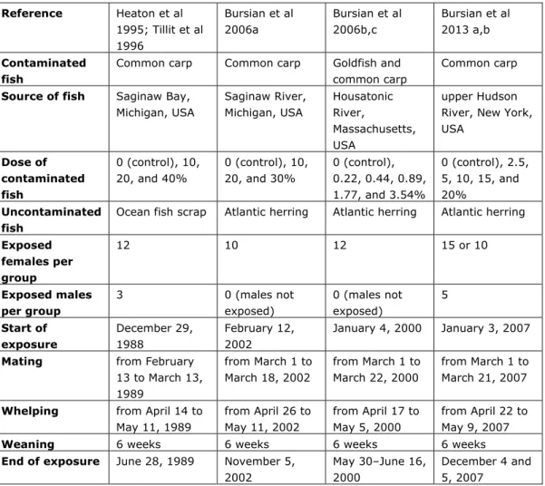
(16) RIVM report 2014-0119. considerable amount of PCBs, especially the toxic planar PCBs, through lactation (Leonards et al. 1996, Smit et al. 1996a, Smit et al. 1996b). A study was performed in which mink were fed with diets containing increasing amounts of contaminated carp from Saginaw Bay instead of uncontaminated marine fish (Heaton et al. 1995, Tillitt et al. 1996). Details for this study and the following studies are summarised in Table 2.1. The study lasted for 182 days, during which period the mink reproduced and nursed the kits. Adults were necropsied after 182 days for organ analysis, including analysis of PCBs in the liver. The survival and body weight of the kits were monitored until six weeks of age (weaning). The survival of the kits at the study’s termination (6 weeks old) was the most sensitive endpoint in the study. In the control group, 85% of the kits survived. In the 10%, 20% and 40% carp diets, 28, 11, and 0% of the kits survived. Thus, a very steep dose-response curve was observed, from which an EC10 (effect concentration) can be obtained with reasonable certainty. Table 2.1 Overview of four toxicity studies involving mink (Mustela vison) given different diets containing fish contaminated with PCBs. Reference. Heaton et al. Bursian et al. Bursian et al. Bursian et al. 1995; Tillit et al. 2006a. 2006b,c. 2013 a,b. Goldfish and. Common carp. 1996 Contaminated. Common carp. Common carp. fish Source of fish. common carp Saginaw Bay,. Saginaw River,. Housatonic. upper Hudson. Michigan, USA. Michigan, USA. River,. River, New York,. Massachusetts,. USA. USA Dose of. 0 (control), 10,. 0 (control), 10,. 0 (control),. 0 (control), 2.5,. contaminated. 20, and 40%. 20, and 30%. 0.22, 0.44, 0.89,. 5, 10, 15, and. fish Uncontaminated. 1.77, and 3.54%. 20%. Ocean fish scrap. Atlantic herring. Atlantic herring. Atlantic herring. 12. 10. 12. 15 or 10. 5. fish Exposed females per group Exposed males. 3. per group. 0 (males not. 0 (males not. exposed). exposed) January 4, 2000. January 3, 2007. Start of. December 29,. February 12,. exposure. 1988. 2002. Mating. from February. from March 1 to. from March 1 to. from March 1 to. 13 to March 13,. March 18, 2002. March 22, 2000. March 21, 2007. from April 14 to. from April 26 to. from April 17 to. from April 22 to. May 11, 1989. May 11, 2002. May 5, 2000. May 9, 2007. Weaning. 6 weeks. 6 weeks. 6 weeks. 6 weeks. End of exposure. June 28, 1989. November 5,. May 30–June 16,. December 4 and. 2002. 2000. 5, 2007. 1989 Whelping. The study results can be expressed in several metrics: as a dose or a diet concentration (diet as such or caloric content) or as internal liver concentration, and as TEQ or as ∑PCB. This will facilitate the calculation of the reference values for PCBs according to the newly developed method for secondary poisoning based on the energy content of the diet (Verbruggen, 2014). However, it will Page 14 of 64.

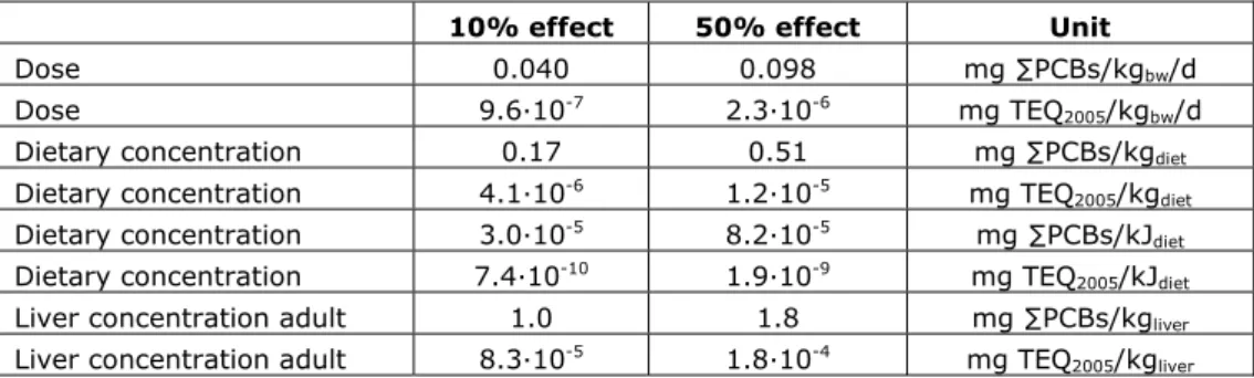
(17) RIVM report 2014-0119. also facilitate the comparison of the toxicity observed for the mink with that for the otter, as will be shown below. The different ways to express the 10% effect level are shown in Table 2.2. Because the composition of the PCB mixtures is given, the data on TEQ can be recalculated using the most recent TEF values (Van den Berg et al. 2006). It should be noted that compounds other than PCBs (polychlorinated dibenzodioxins (PCDDs) and polychlorinated dibenzofurans (PCDF)) do contribute to the overall TEQ as well. PCDDs and PCDF made up 9%, 37%, 26% and 28% of the recalculated TEQ in the control, with 10%, 20% and 40% carp diets, respectively. Table 2.2 10% and 50% effect levels for the survival of mink kits up to 6 weeks of age in the study using contaminated fish from Saginaw Bay (Heaton et al. 1995). Values are expressed in different metrics that are relevant for the assessment of secondary poisoning. 10% effect. 50% effect. Unit. Dose. 0.040. 0.098. mg ∑PCBs/kgbw/d. Dose. 9.6·10-7. 2.3·10-6. mg TEQ2005/kgbw/d. Dietary concentration. 0.17. 0.51. mg ∑PCBs/kgdiet. Dietary concentration. 4.1·10-6. 1.2·10-5. mg TEQ2005/kgdiet. Dietary concentration. 3.0·10-5. 8.2·10-5. mg ∑PCBs/kJdiet. 1.9·10-9. mg TEQ2005/kJdiet. Dietary concentration. -10. 7.4·10. Liver concentration adult. 1.0. 1.8. mg ∑PCBs/kgliver. Liver concentration adult. 8.3·10-5. 1.8·10-4. mg TEQ2005/kgliver. In a second study, carp from the Saginaw River at Bay City, Michigan was added to the diet (Bursian et al, 2006a). The fraction was similar to the first study (10-30% contaminated fish). Males were not exposed. The time between the start of the exposure and the beginning of mating was shorter than in the other studies. In this study too, the composition of the PCB mixtures was given and the TEQ was recalculated using the most recent TEF values (Van den Berg et al., 2006). PCDDs and PCDF made up 94%, 62%, 63% and 60% of the recalculated TEQ in the control, with 10, 20, and 30% carp diets, respectively. The contribution of the non-ortho PCB 126 to the TEQ was around 32% in the contaminated fish, and of the mono-ortho PCB 118 3%. Body weight and food consumption were not given in this study. Consequently, no dose could be derived from the data. The study presented the nutritional information and, therefore, diet concentrations can be expressed on an energy basis. In this study, no effects on survival were found up to the highest concentration. The results are presented in Table 2.3. The lack of effects on survival starkly contrasts with the study from Saginaw Bay (Heaton et al. 1995; Tillit et al. 1996), in which strong effects were observed at equivalent TEQ. The authors indicate that the fish in the present study contain relatively high amounts of PCDDs and PCDFs. They point to the limitations of the TEQ approach, which assumes additivity, while antagonistic and synergistic effects may occur. The fact that the males were not exposed in this study is also considered to be an explanatory factor by the authors. Based on their subsequent studies (Bursian et al. 2006b,c; Bursian et al. 2013a,b), this may indeed be a relevant factor. In the study, in which male mink were not exposed (Bursian et al. 2006b,c), effect levels were higher than in the other two studies. Furthermore, the exposure time before mating is not mentioned by the authors, but this appeared to have been significantly shorter than in the other studies. In Table 2.1 the study details for all studies are compared. Page 15 of 64.

(18) RIVM report 2014-0119. Table 2.3 No observed effect and lowest observed effect levels for the survival of mink kits up to 6 weeks of age in the study using contaminated fish from the Saginaw River (Bursian et al. 2006a). Values are expressed in different metrics that are relevant for the assessment of secondary poisoning. No effect. Lowest. Unit. observed effect Dietary concentration. 1.7. >1,7. mg ∑PCBs/kgdiet. Dietary concentration. 5.7·10-5. >5.7·10-5. mg TEQ2005/kgdiet. Dietary concentration. 2.1·10-4. >2.1·10-4. mg ∑PCBs/kJdiet. Dietary concentration. -9. 7.1·10. >7.1·10-9. mg TEQ2005/kJdiet. Liver concentration 6-w kit. 19. >19. mg ∑PCBs/kgliver. Liver concentration 6-w kit. 2.4·10-4. >2.4·10-4. mg TEQ2005/kgliver. Liver concentration 27-w kit. 18. >18. mg ∑PCBs/kgliver. Liver concentration 27-w kit. 7.8·10-5. >7.8·10-5. mg TEQ2005/kgliver. A third study examined the toxicity of fish from the Housatonic River in Massachusetts (Bursian et al. 2006b,c). The study was very similar to the former one. In this study, as well, males were not exposed. The fraction of contaminated fish was much lower in this study due to the higher contamination. Again, kit mortality after 6 weeks was the most sensitive endpoint relevant for reproduction. Survival was only affected in the highest dose. In this study, too, the composition of the mixtures was given and the TEQ was recalculated using the most recent TEF values (Van den Berg et al. 2006). PCDDs and PCDF made up 39%, 19%, 13%, 9%, 6% and 6% of the recalculated TEQ in the control, with 0.22, 0.44, 0.89, 1.77 and 3.54% carp/goldfish diets, respectively. The contribution of the non-ortho PCBs to the TEQ was around 88% in the contaminated fish, with PCB126 alone accounting for around 81%. Table 2.4 No observed effect and lowest observed effect levels for the survival of mink kits up to 6 weeks of age in the study using contaminated fish from the Housatonic River (Bursian et al. 2006b,c). Values are expressed in different metrics that are relevant for the assessment of secondary poisoning. No effect. Lowest observed effect. Unit. Dose. 0.169. 0.414. mg ∑PCBs/kgbw/d. Dose. 9.6·10-7. 2.3·10-6. mg TEQ2005/kgbw/d. Dietary concentration. 1.6. 3.7. mg ∑PCBs/kgdiet. Dietary concentration. 1.2·10-5. 5.0·10-5. mg TEQ2005/kgdiet. Liver concentration adult. 3.08. 3.13. mg ∑PCBs/kgliver. Liver concentration adult. 5.0·10-5. 1.9·10-4. mg TEQ2005/kgliver. Liver concentration 6-w kit. 1.9. 3.7. mg ∑PCBs/kgliver. Liver concentration 6-w kit. 7.7·10-5. 1.7·10-4. mg TEQ2005/kgliver. Liver concentration 31-w kit. 3.5. 8.6. mg ∑PCBs/kgliver. Liver concentration 31-w kit. 7.7·10-5. 1.5·10-4. mg TEQ2005/kgliver. A similar, but more recent study was performed with mink fed with contaminated food from the upper Hudson River (Bursian et al. 2013). In this study, the contribution of PCBs to the total TEQ in the diet was 97%, with nonortho-PCBs accounting for 75% and PCB126 for 74%. Thus, PCB126 was by far the most important congener for the total TEQ. In the livers of the female mink, these percentages increased to 98%, 82% and 82%, respectively. The lowest Page 16 of 64.

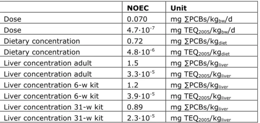
(19) RIVM report 2014-0119. diet concentration is considered as NOEC (No Observed Effect Concentration). It should be noted that, if the number of kits whelped alive per dam is multiplied by the chance of surviving up to six weeks of age (point of weaning) and then by the chance of surviving from the point of weaning to 31 weeks of age, there is still an effect of 23% compared with the control. At all higher concentrations, none of the kids survived up to 31 weeks of age, pointing to a very steep doseresponse relationship. Besides the steep dose-response relationship, the number of kits alive per dam was probably not impacted at the lowest exposure concentration, because it was higher than the control in the next exposure concentration. This leaves an increased mortality from birth until the end of the study of around 15% compared with the control group (there appears to be some inconsistencies between text, tables and figures). With this value being close to 10% and in view of the steep dose-response, it is further considered as a NOEC. It should be noted that at six weeks of age the effect on mortality was not significant in the next higher concentration either. However, the body weight of the kits was significantly reduced at this concentration and higher concentrations at both three and six weeks of age. For a comparison with the other studies, the data based on kit mortality at six weeks of age are presented in Table 2.5. Table 2.5 No observed effect and lowest observed effect levels for the survival of mink kits up to 6 weeks of age in the study using contaminated fish from the upper Hudson River (Bursian et al. 2013a,b). Values are expressed in different metrics that are relevant for the assessment of secondary poisoning. No effect. Lowest. Unit. observed effect Dose. 0.15. 0.27. mg ∑PCBs/kgbw/d. Dose. 9.7·10-7. 1.7·10-6. mg TEQ2005/kgbw/d. Dietary concentration. 1.5. 2.8. mg ∑PCBs/kgdiet. Dietary concentration. 1.0·10-5. 1.8·10-5. mg TEQ2005/kgdiet. Liver concentration adult. 2.9. 3.4. mg ∑PCBs/kgliver. Liver concentration adult. 6.1·10-5. 1.0·10-4. mg TEQ2005/kgliver. The more sensitive NOEC values for juvenile mortality (kit at 31 weeks of age) will be used in the derivation of the risk limits. These no observed effect levels are presented in Table 2.6. Table 2.6 No observed effect levels for the survival of mink kits up to 31 weeks of age in the study using contaminated fish from the upper Hudson River (Bursian et al. 2013a,b). Values are expressed in different metrics that are relevant for the assessment of secondary poisoning. NOEC. Unit. Dose. 0.070. mg ∑PCBs/kgbw/d. Dose. 4.7·10-7. mg TEQ2005/kgbw/d. Dietary concentration. 0.72. mg ∑PCBs/kgdiet. Dietary concentration. 4.8·10-6. mg TEQ2005/kgdiet. Liver concentration adult. 1.5. mg ∑PCBs/kgliver. Liver concentration adult. 3.3·10-5. mg TEQ2005/kgliver. Liver concentration 6-w kit. 1.2. mg ∑PCBs/kgliver. Liver concentration 6-w kit. 3.9·10-5. mg TEQ2005/kgliver. Liver concentration 31-w kit. 0.89. mg ∑PCBs/kgliver. Liver concentration 31-w kit. 2.3·10-5. mg TEQ2005/kgliver Page 17 of 64.

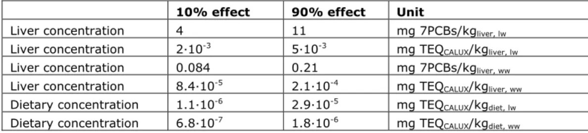
(20) RIVM report 2014-0119. A dose-response relationship was developed between liver vitamin A content and liver concentrations of PCBs in otters (Lutra lutra) that were found dead in the Netherlands (Murk et al. 1998). It appeared that there was a very sharp doseresponse relationship, especially with the TEQ as determined by the CALUX assay. The data are based on measured concentrations in the liver. Data based on the sum of seven indicator PCBs were estimated on the basis of relationships between seven indicator PCBs and TEQ (Smit et al. 1996a). On the basis of the same study, a translation to a concentration in fish was made (Murk et al. 1998), which is also shown in Table 2.7. Table 2.7 Levels corresponding to 10% and 90% reduction in vitamin A levels in livers from otters. 10% effect. 90% effect. Liver concentration. 4. 11. mg 7PCBs/kgliver, lw. Liver concentration. 2·10-3. 5·10-3. mg TEQCALUX/kgliver, lw. Liver concentration. 0.084. 0.21. mg 7PCBs/kgliver, ww. Liver concentration. 8.4·10-5. 2.1·10-4. mg TEQCALUX/kgliver, ww. Dietary concentration. 1.1·10-6. 2.9·10-5. mg TEQCALUX/kgdiet, lw. Dietary concentration. -7. 1.8·10-6. mg TEQCALUX/kgdiet, ww. 6.8·10. Unit. It can be concluded based on a comparison of Tables 2.1 - 2.7 that, especially for the liver concentrations based TEQ concentration (on wet weight), there is a very good correspondence between the effect range in mink and otter:  8.3·10-5 and 1.8·10-4 mg TEQ2005/kgliver in the livers of adult females correspond to 10 and 50% effect in kit mortality at six weeks of age in the first study using fish from Saginaw Bay, and  2.4·10-4 and 7.8·10-5 mg TEQ2005/kgliver in liver of 6-week and 27-week old kits in the highest tested concentration correspond to no effect in kit mortality at six weeks of age in the second study using fish from the Saginaw River, and  5.0·10-5, 7.7·10-5 and 7.7·10-5 mg TEQ2005/kgliver in the liver of an adult female, 6-week and 27-week old kits correspond to no effect in kit mortality at six weeks of age in the third study using fish from the Housatonic River, while 1.9·10-4, 1.7·10-4 and 1.5·10-4 mg TEQ2005/kgliver corresponded to increased mortality for six-week old kits, and  6.1·10-5 mg TEQ2005/kgliver in the liver of an adult female corresponds to the NOEC for kit mortality at six weeks of age in the fourth study for the mink using fish from the upper Hudson River, while 1.0·10-4 mg TEQ2005/kgliver corresponded to an increased mortality at six weeks of age; for the mortality of kits at 31 weeks of age, liver concentration that resulted in no effects were as low as 3.3·10-5 , 3.9·10-5, 2.3·10-5 mg TEQ2005/kgliver in the liver of an adult female, 6-week and 31-week old kits, respectively, and  8.4·10-5 to 2.1·10-4 mg TEQCALUX/kgliver marked the range of liver concentrations corresponding to a 10 to 90% decrease in hepatic vitamin A concentrations in the otter. On the basis of these results, it can be concluded that mink and otter have a similar sensitivity to the toxicity of dioxin-like compounds, such as PCBs. 2.3. Biomagnification Biomagnification expresses the accumulation of substances from lower trophic levels in the food chain to the predators. For an assessment of the exposure of terrestrial predators to these substances, the magnification in the terrestrial Page 18 of 64.

(21) RIVM report 2014-0119. food chain should be known. Biomagnification in mustelids, including the otter, and the rest of the terrestrial predators is described in this section. 2.3.1. Biomagnification in otters In the 1990s, quality objectives for PCBs were developed based on the toxicity for the otter (Lutra lutra), which is considered as a sentinel species, and its closely related relative, the mink (Traas et al. 2001; Smit et al 1996c). Because the quality objectives for otters are based on internal effect concentrations in otter livers, the biomagnification from fish to otters is a key parameter in the derivation of these objectives. The biomagnification factors used are remarkably high, especially for the planar PCBs and consequently also for the TEQ (Smit et al. 1996a, Leonards et al. 1997). The biomagnification studies used for this purpose, however, have some shortcomings. In both studies, the otter samples pre-dated the fish samples by several years. It is necessary, therefore, to verify whether the quality objectives for PCBs derived for the otter (Traas et al. 2001) are not too stringent because of the use of excessively high BMF values, especially for the planar non-ortho substituted PCBs. In the Danish habitat (only freshwater lakes were used by Traas et al. 2001), fish were sampled in the period April-June 1995. Sediment was sampled concurrently. The nine otters (five males, four females) were retrieved from a database and were from 1988 or later (Smit et al. 1996a). In the Dutch habitat, (freshwater lakes) sediment and invertebrates were sampled in June 1993. Fish samples of several species were collected from June 1990 to January 1991. The otters were found dead between 1982 and 1988 and were the last five dead otters found in the Netherlands. Apparently, they are not from the same location as the fish, although all were from the northern part of the Netherlands. Besides that, arithmetic means of concentrations have been used for the prey items, while the geometric mean was calculated for the otters. It is suggested that PCB77 is metabolized by otters because its relative contribution to the TEQ decreases from fish to otter and that PCB126 and PCB169 are increased due to selective retention. The authors conclude from the literature that this specific retention is not observed for other mammals and birds besides the otter (Leonards et al. 1997). Geometric means of lipid normalized concentrations do not show a decrease from fish to otter for PCB77, but there is very strong increase for PCB126 and PCB169. As can be concluded, the temporal scale between the sampling of fish and the otters is large, which makes the resulting biomagnification factors less reliable. In the Dutch study as well, the spatial scale for the sampling is substantial, which makes the biomagnification parameters even less certain. Besides that, the otter itself is a migratory species, which makes it more complicated to link it to a diet in a restricted area. Especially the temporal aspect may lead to erroneously high BMF values if the prey species are sampled several years after the predator species in cases of declining environmental concentrations. With regard to this aspect, it is noteworthy that reductive dechlorination, especially, removes meta and para chlorine atoms which strongly reduce the non-ortho PCBs (i.e. PCB126 and PCB 169) with relatively short half-lives of 6 years, as assumed in the modelling exercises (Traas et al., 2001). On the contrary, it is stated that the concentration and profiles of PCBs have not markedly changed in the Netherlands (Leonards et al. 1998). Besides that, the BMF values obtained Page 19 of 64.

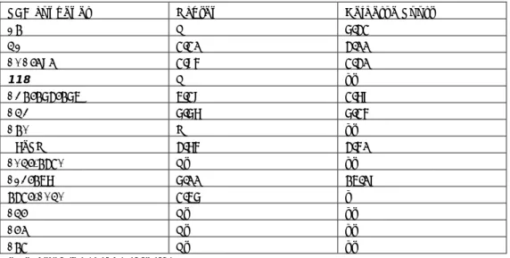
(22) RIVM report 2014-0119. from the Danish otters (Smit et al. 1996a) and from the Dutch otters (Leonards et al. 1997) show the same pattern, with the highest BMFs observed for the planar PCBs. 2.3.2. Biomagnification in other mustelids in comparison with otters A similar biomagnification study was performed for other mustelids. Weasels (Mustela nivalis; 6 animals, 4 males; 2 females), stoats (Mustela erminea; 7 animals, 4 males; 3 females), and polecats (Mustela putorius; 4 animals, 1 male; 3 females) were collected in the period between 1985 and 1993 from the Oude Venen area or within a radius of 7 km (Leonards et al. 1998). The prey species of these terrestrial mustelids were sampled in 1993 in the Oude Venen or in the surrounding area. These prey species consisted of red vole (Clethrionomys glareolus), common vole (Microtus arvalis), wood mouse (Apodemus sylvaticus), common shrew (Sorex araneus), common hare (Lepus europaeus), common frog (Rana temporaria), lake frog (Rana esculenta), common toad (Bufo bufo), and natterjack (Bufo calamita). All mustelids are able to metabolize PCBs with vicinal hydrogen atoms in the meta and para position. Evidence for this comes also from the fact that methylsulphonyl metabolites of these congeners were detected in the liver of various mustelids. Only metabolites of PCB149 were detected in all mustelid species. Metabolites of other congeners were mainly restricted to the otters. Besides that, concentration ratios of the methylsulphonyl metabolites to the parent compound PCB149 were far higher for otters than for the other mustelid species. This is also confirmed by the fact that biomagnification factors for these congeners are much lower in otters than in the other mustelids. It is suggested that only polecats are able to metabolize PCB congeners with five or more chlorine atoms and vicinal hydrogen atoms on the ortho and meta position, such as PCB126. This is deduced from the fact that for polecats the ratio of PCB126 to PCB153 is much lower than it is for the other mustelids. For these other mustelid species, it is suggested that these PCB congeners, such as 126 and 169, are selectively retained in the liver. However, the biomagnification factor for this PCB congener 126 is among the highest for polecats in comparison with the other mustelids. The biomagnification factor for PCB153 and other non-metabolisable congeners is moreover much higher for polecats than it is for the other mustelids. A closer look at the data shows that the relatively low amount of PCB126 in liver of polecats might be partly related to the food items as well. It appears that amphibians contain a much lower amount of PCB126 and the other co-planar PCBs in comparison with other prey organisms. Polecats are the only mustelids that eat substantial amounts of amphibians. In the diet used to calculate the biomagnification factors, this amount was 20%. Yet this was not determined in the study itself, but rather from older data taken from another location and the Oude Venen location from this study is a marsh type of landscape. Data from this study are analysed here for their relative amount of TEQ. The low amount of PCB126 and other coplanar PCBs in amphibians is reflected in the low TEQ value of the PCBs.. Page 20 of 64.

(23) RIVM report 2014-0119. Polecat Weasel Stoat Otter Amphibians Mammals Fish -6. -5. -4. -3. -2. log (TEQ/ PCB) Figure 2.1 Ratio of TEQ values to total PCBs for various species of mustelids and some groups of prey items from the Oude Venen area (data from Leonards et al. 1997, 1998). Filled symbols refer to males for the terrestrial mustelids. Another interesting aspect is the fact that, in the case of stoat and weasel, more than half of the individuals were males, while in the group of polecats there was only one male. For both weasel and stoat, it appeared that the males had relative TEQ concentrations compared with the sum of PCBs that were about twice those of females. For polecats, there is only one male and therefore a meaningful comparison is impossible, especially due to the large variation in the ratio between TEQ and the sum of PCBs. A possible explanation for this large variation up to a factor of 14 could be a difference in diet of the polecat as discussed above. The study on otters did not address the difference between male and female otters explicitly, although the differences caused by lactation were recognized (Leonards et al. 1996; Smit et al. 1996a; Smit et al. 1996b). For the Dutch habitat, the gender of the otters was not given at all (Leonards et al. 1997). For the Danish habitat, the gender and life stage was reported and in the appendix BMF values were given separately for male and female otters. On a TEQ basis, the BMF was 174 for males and 44 for females, while the geometric mean was 95 (Smit et al. 1996a). This means that the data for the stoat and weasel are in line with the data for the otter. In a laboratory toxicity study with mink (Mustela vison), the accumulation of PCBs was determined as well (Tillitt et al. 1996). In such a study, diet concentrations are controlled and the concentration in mink can be directly coupled to the concentrations in the diet. In this way, temporal and spatial variation, as encountered in the field studies, is eliminated. In line with the studies for other mustelids, biomagnification factors were highest for the planar PCB congeners 126 and 169 in comparison with total PCBs (BMF = 8-15 for PCB126 and 12-21 for PCB169 in comparison with 2.4-3.9 for ∑PCB, based on Aroclor standards). Leonards et al. (1998) stated that there was no explanation for the fact that the BMFs for PCB126 were much higher in stoat and otter than they were in mink. However, it should be noted that not only PCB126 but all PCBs had lower biomagnification factors in the mink. There are two plausible explanations for this. First, the mink had been exposed in captivity for a limited exposure time of 182 days, while feral mustelids were exposed their whole life long. Perhaps even more important, however, is the fact that the mink that were Page 21 of 64.

(24) RIVM report 2014-0119. analysed were lactating females. Nursing is known to have a dramatic decreasing effect on the PCB concentration in the parent female (Leonards et al. 1996; Smit et al. 1996a; Smit et al. 1996b). 2.3.3. Biomagnification from earthworms to shrews In a field study, earthworms and shrews were sampled from two different locations in the Kalamazoo River floodplain (Blankenship et al., 2005). One area, Fort Custer State Recreation Area (FC), was a reference site and the other area, Former Trowbridge Impoundment (TB), was a contaminated site. Not all congeners were separated from each other, but the indicator PCBs mostly dominated the non-separated peaks. The BMFs were calculated for the different congeners, including the indicator PCBs, the sum of the seven indicator-PCBs (∑7PCB), the planar PCBs and the sum of the TEQ. For both sites, the worms were rinsed and directly determined (fresh) or allowed to clear their gut for 24 to 48 hours (depurated). In Table 2.8 only the values for the indicator PCBs and the planar PCBs are given. Table 2.8 Lipid-normalized biomagnification factors from earthworms to shrews taken from two sites; Fort Custer reference site, Trowbridge contaminated site, in the Kalamazoo River floodplain (Blankenship et al. 2005). Indicator PCBs are given in bold, (co)planar PCBs are given in italics. PCB congener. Fort Custer. Trowbridge. Fresh. Depurated. Fresh. 28,31. 0.45. 0.02. 0.15. Depurated 0.20. 52. 5.68. 0.74. 0.04. 0.06. 56,92,84,90,101,113. 3.39. 0.80. 0.06. 0.10. 118. 1.62. 0.45. 2.40. 2.72. 138, 158. 1.09. 1.29. 2.62. 3.54. 105,132,153. 2.61. 1.90. 3.07. 4.14. 180. 4.53. 7.84. 12.20. 9.45. ∑7PCB. 2.28. 0.96. 0.85. 1.23. 156,171,202,157,201. 42.02. 2.02. 4.35. 6.73. 128, 167,185. 2.27. 5.16. 3.45. 4.04. 77. 0.79. 0.25. 0.07. 0.13. 81. 1.40. 1.51. 0.50. 0.84. 126. 2.94. 1.38. 22.22. 31.85. 169. 1.44. 1.73. 0.68. 2.13. TEQ. 2.63. 1.41. 12.31. 17.53. In a similar study in the Netherlands, soil, earthworm and shrew samples were collected from two flood plain sites of the Rhine delta (Hendriks et al., 1995). Worms were allowed to clear their gut for 24 hours to remove the soil present in the digestive tract. From these data, BMF values can be calculated. The results for the seven indicator PCBs and, if available, the planar PCBs are tabulated in Table 2.9.. Page 22 of 64.

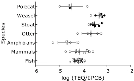
(25) RIVM report 2014-0119. Table 2.9 Lipid-normalized biomagnification factors from earthworms to shrews at two flood plain sites in the Rhine delta (Hendriks et al. 1995). Indicator PCBs are given in bold, (co)planar PCBs are given in italics. PCB congener. Ochten. 28. A. Gelderse Poort 6.32. 52. 2.20. 3.00. 101/090. 2.95. 2.30. 118. A. ab. 138/163/164. 4.29. 2.78. 153. 6.67. 6.25. 180. B. ab. ∑7PCB. 3.75. 3.50. 105/(132). Ab. ab. 123/147. 6.00. 14.08. 132/(105). 2.46. a. 156. Ab. ab. 167. Ab. ab. 189. Ab. ab. a No value for shrews reported b No value for earthworms reported. In another study from the Netherlands (Van den Brink, 2000), the food chain of the little owl was studied in two areas: the Gelderse Poort and the Achterhoek. The data for the Gelderse Poort contained both earthworm and shrew concentrations. BMF values could be derived from these data (Table 2.10). Table 2.10 Lipid-normalized biomagnification factors from earthworms to shrews at two locations in the Gelderse Poort (GP) (Van den Brink, 2000). All PCBs are indicator PCBs, (co)planar PCB 118 is given in italics.. 2.3.4. PCB congener. GP9. GP11. 28. 0.15. 0.18. 52. 0.05. 0.08. 101. 0.04. 0.07. 118. 0.76. 0.08. 138. 0.80. 0.91. 153. 0.41. 0.89. 180. 1.16. 1.67. ∑7PCB. 0.55. 0.78. Biomagnification in other birds and mammals A food web study was performed with tree swallows (Tachycineta bicolor) in the Hudson River area, in New York state, US (Echols et al. 2004). Two of the sites, Remnant Deposit 4 and Special Area 13 are known areas of high PCB contamination. It appeared that congener pattern in food (diptera, collected as food bolus from the swallows), as well as eggs, nestlings, and adult swallows, were different from individual technical Aroclor mixtures, but resembled a combination of Aroclor 1248 and Aroclor 1254 (determined with principle component analysis, PCA). The congener pattern in the eggs was closely related to that in the adults, while that in nestlings was closely related to the food (clusters in the PCA).. Page 23 of 64.

(26) RIVM report 2014-0119. The reported uptake rates from these areas were not equal to the daily dose the nestlings received with the food, because uptake efficiency, metabolism, and elimination also played a role. Metabolism was relatively unimportant, given the fact that the congener patterns in food and nestlings were comparable. However, elimination over 10 days may account for a significant difference between these values and the daily dose received. It is stated that the use of a biomagnifcation factor in this case was not appropriate, because the nestlings were far from a steady state. Indeed, from the supporting information, it is evident that the total lipid normalized PCB concentrations in 5-d, 10-d and 15-d old nestlings was only 7, 12 and 15% of that of adult birds, who might have been exposed elsewhere as well, yet 0.9, 1.5 and 1.9 times higher than the lipid normalized concentration in food (diptera), respectively. This shows that, indeed, the biomagnification process was not in a steady-state after 15 days. The ratio of the seven indicator PCBs as a fraction of total PCBs (103 peaks, 121 congeners) appeared to be rather constant over all four sampling sites and over all biota, varying between 20 and 34%. However, eggs and adults seemed to have a somewhat higher content of indicator PCBs. This was also observed for all samples from the site at Champlain Canal, which is located upstream from the contaminated sites. These eight samples had an average percentage of 31% indicator PCBs. The lower percentages of indicator PCBs might, therefore, be representative of this particular contamination. In another food web study involving tree swallows (Papp et al. 2007), the samples were analysed for 85 congeners. Sixty-six congeners were detected, 59 of which were detected in all nestling samples. In the two groups of insects, Hexagenia and Chironomidae, only 53 and 34 congeners were detected, respectively. Of the seven indicator-PCBs, PCB 28 was not reported, so the sum derived from this study was based on the remaining six congeners. The ratio between the 13-d old nestlings and insects (hexagenia and chironimidae) varied between 0.55 and 1.61 for the six congeners, with a value of 1.05 for the sum of the six congeners. These values were slightly lower than in the other study involving tree swallows. No time trend was available from this study. In a study that examined the magnification from food to great tits (Parus major), it appeared that the main food item for the nestlings (caterpillars) was not the most important source for PCBs, but rather maternal transfer to the eggs. As concentrations of nestlings decreased instead of increased with age, the ratio between PCB concentration in nestlings and caterpillars was not considered to be a good metric for biomagnification (Dauwe et al. 2006). In this study, a total of 22 PCBs were analysed. Of the seven indicator PCBs, PCB 28, PCB 52 and PCB 118 were not reported, but probably belonged to the set of 22 congeners. Based on the studies involving the nestlings of tree swallows and great tits, it appears that the biomagnification was not necessarily representative of the exposure from local food sources, as is reflected by the important role played by the transfer from adult to eggs, the build-up of or the decrease in nestling concentrations dependent on the situation, and the observed variability in congener pattern between adults, eggs and nestlings. These biomagnification studies, therefore, appear to be rather unsuitable for assessing the transfer of PCBs from local soil sources to birds. Page 24 of 64.

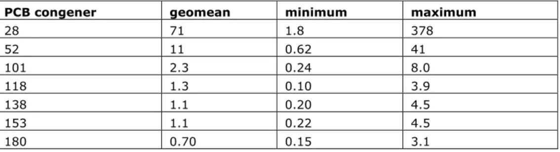
(27) RIVM report 2014-0119. Reported biomagnification factors for PCB congeners between passerine birds and sparrowhawks were around 20, and BMF between rodents and buzzards were around 40, whereas BMF between rodents and fox were somewhat lower (BMF around 3). Woodmouse (Apodemus sylvaticus) and bank vole (Clethrionomys glareolus) were sampled around Antwerp in February and March 2001. The great tits were sampled around Antwerp between 2001 and 2003 (Voorspoels et al. 2007). The foxes (Vulpes vulpes) were from the south of Belgium and were sampled between October 2003 and March 2004 (Voorspoels et al. 2006a), while the buzzards (Buteo buteo) and the sparrowhawks (Accipiter nisus) were from the eastern part of Flanders and were sampled between November 2001 and March 2003 (Voorspoels et al. 2006b). Therefore, the reliability of these BMF values can be argued because prey and predators are not from the same ecosystem. 2.4. Terrestrial bioaccumulation Bioaccumulation in soil is described by biota-to-soil-accumulation-factors (BSAF), which express the ratio of the concentrations of a substance in terrestrial organisms to its concentration in soil. To make a link between the concentrations in the prey organisms for terrestrial predators and the concentration in the soil, the bioaccumulation in terrestrial species must be known. Bioaccumulation from soil in terrestrial species is described in this section.. 2.4.1. Bioaccumulation from soil to earthworms Earthworms (Lumbricus terrestris L.) were exposed to 25 different soils for 15 days (Krauss et al. 2000). The soils were from Bavaria, Germany, and covered a wide range of land use and texture. Preliminary experiments with three soils showed that 15 days was sufficient to approach equilibrium. The worms were allowed to purge their gut for 48 hours on wet filter paper. The BSAF were not given for each soil separately, but presented in a figure with mean, minimum and maximum values. The values that were derived are presented in Table 2.11. Only the values for the seven indicator PBCs are presented here. Table 2.11 Lipid and organic carbon normalized BSAF values for earthworms in 25 soils from Germany (Krauss et al. 2000). PCB congener. geomean. minimum. maximum. 28. 71. 1.8. 378. 52. 11. 0.62. 41. 101. 2.3. 0.24. 8.0. 118. 1.3. 0.10. 3.9. 138. 1.1. 0.20. 4.5. 153. 1.1. 0.22. 4.5. 180. 0.70. 0.15. 3.1. In a field study, soil and earthworms were sampled from two different locations in the Kalamazoo River floodplain (Blankenship et al. 2005). One area, Fort Custer State Recreation Area (FC), was a reference site and the other area, Former Trowbridge Impoundment (TB), was a contaminated site. Not all congeners were separated from each other, but the indicator PCBs mostly dominated the non-separated peaks. The BSAFs were calculated from the presented concentrations for the different congeners, including the indicator PCBs, the sum of the seven indicator-PCBs, the planar PCBs and the sum of the Page 25 of 64.

(28) RIVM report 2014-0119. TEQ. For both sites, the worms were rinsed and directly determined (fresh) or allowed to clear their gut for 24 to 48 hours (depurated). In Table 2.12, only the values for the indicator PCBs and the planar PCBs are given. Table 2.12 Lipid and organic carbon normalized BSAF values for earthworms taken from two sites; Fort Custer reference site, Trowbridge contaminated site in the Kalamazoo River floodplain (Blankenship et al. 2005). Indicator PCBs are given in bold, (co)planar PCBs are given in italics. PCB congener. Fort Custer. Trowbridge. Fresh. Depurated. Fresh. Depurated. 28,31. 0.31. 5.72. 0.61. 0.46. 52. 0.33. 2.54. 0.98. 0.69. 56,92,84,90,101,113. 1.42. 6.02. 0.84. 0.49. 118. 0.83. 3.01. 0.50. 0.44. 138, 158. 2.05. 1.73. 0.77. 0.57. 105,132,153. 1.56. 2.15. 0.58. 0.43. 180. 1.47. 0.85. 0.25. 0.32. ∑7PCB. 1.31. 3.12. 0.75. 0.52. 156,171,202,157,201. 0.10. 2.04. 0.34. 0.22. 128, 167,185. 0.77. 0.34. 0.35. 0.29. 77. 1.41. 4.44. 0.42. 0.23. 81. 2.67. 2.47. 0.55. 0.33. 126. 2.02. 4.31. 0.29. 0.20. 169. 3.10. 2.59. 6.31. 2.01. TEQ. 2.14. 4.01. 0.38. 0.27. In a similar study in the Netherlands, soil and earthworm samples were collected from two flood plain sites in the Rhine delta. Worms were allowed to clear their gut for 24 hours to remove the soil present in the digestive tract. The results for the seven indicator PCBs and some (co)planar PCBs are tabulated in Table 2.13. Table 2.13 Lipid and organic carbon normalized BSAF values for earthworms taken from two flood plain sites in the Rhine delta (Hendriks et al. 1995). Indicator PCBs are given in bold, (co)planar PCBs are given in italics. PCB congener. Ochten. 28. b. Gelderse Poort 0.16. 52. 0.69. 0.20. 101/090. 0.61. 0.31. 118. 0.53. A. 138/163/164. 0.51. 0.35. 153. 0.39. 0.20. 180. a. A. ∑7PCB. 0.45. 0.24. 105/(132). a. A. 123/147. 0.96. 0.42. 132/(105). 0.55. 0.32. 156. a. A. 167. a. A. 189. a. A. a No value for earthworms reported b No value for soil reported. Page 26 of 64.

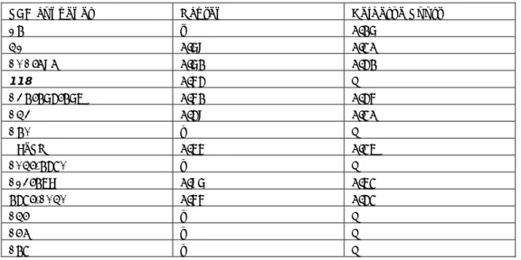
(29) RIVM report 2014-0119. In another study from the Netherlands (Van den Brink, 2000), the food chain of the little owl was studied in two areas: the Gelderse Poort and the Achterhoek. The data for the Gelderse Poort contained both soil and earthworm concentrations. BSAF values could be derived from these data (Table 2.14). Table 2.14 Lipid and organic carbon normalized BSAF values for earthworms from four sites in the Gelderse Poort (GP) floodplain (Van den Brink, 2000). PCB congener. GP1. GP9. GP11. K15. 28. 0.50. 0.29. 0.17. 0.31. 52. 2.42. 1.45. 0.65. 0.92. 101. 3.68. 2.54. 1.44. 1.17. 118. 0.58. 0.37. 0.74. 0.55. 138. 3.73. 3.43. 1.73. 1.60. 153. 3.98. 4.22. 1.50. 1.18. 180. 2.42. 2.30. 1.18. 0.90. ∑7PCB. 2.87. 2.53. 1.27. 1.09. Another field study examined the uptake of worms in open woodland and grassland from two sites near the city of Antwerp in Belgium (Vermeulen et al., 2010). No gut depuration of the earthworms was allowed. The BSAF values calculated from these data are presented in Table 2.15. Table 2.15 Lipid and organic carbon normalized BSAF values for earthworms taken from two sites near the city of Antwerp (Vermeulen et al. 2010). PCB congener. geomean. minimum. maximum. Brasschaat grassland 101. 1.29. 0.79. 1.88. 118. 0.58. 0.36. 0.85. 138. 0.61. 0.37. 0.88. 153. 0.61. 0.37. 0.88. 180. 0.58. 0.36. 0.85. ∑PCB (10 congeners). 1.05. 0.64. 1.53. Brasschaat open woodland 101. 2.31. 1.60. 4.99. 118. 1.35. 0.94. 2.93. 138. 1.64. 1.14. 3.55. 153. 1.40. 0.97. 3.03. 180. 1.71. 1.18. 3.70. ∑PCB (10 congeners). 2.55. 1.76. 5.51. Hoboken grassland 101. 1.22. 0.43. 2.65. 118. 0.55. 0.19. 1.19. 138. 0.57. 0.20. 1.25. 153. 0.57. 0.20. 1.25. 180. 0.55. 0.19. 1.19. 0.99. 0.35. 2.15. ∑PCB (10 congeners). Hoboken woodland 101. 0.68. 0.49. 1.00. 118. 0.40. 0.29. 0.59. 138. 0.49. 0.35. 0.71. 153. 0.42. 0.30. 0.61. 180. 0.51. 0.36. 0.74 Page 27 of 64.

(30) RIVM report 2014-0119. PCB congener. geomean. minimum. maximum. ∑PCB (10 congeners). 0.75. 0.54. 1.10. Another study from China didn’t specify the soil type and both earthworm and soil concentrations were given on the basis of dry weight (Zhao et al. 2006). The BSAF values that were derived from these concentrations are given in Table 2.16. Table 2.16 Dry-weight-based BSAF values for earthworms taken from a polluted farmland (Zhao et al., 2006). Indicator PCBs are given in bold, (co)planar PCBs are given in italics. PCB congener. WenTai area, Zhejiang Province of China. 28. 5.3. 52. 8.4. 101. 12.2. 118. 7.6. 138. 21.7. 153. 16.9. 180. 12.9. ∑7PCB. 8.1. 77. 2.4. 81. A. 105. 6.6. 114. 16.6. 126. 4.4. 156. 13.1. 157. 10.7. 167. 10.2. 169. B. 189. 4.9. WHO-TEQ (probably 1998). 4.8. a Worm concentration below detection limit b Both worm and soil concentrations below detection limit. With standard values (Jager, 1998) for the lipid content and dry-weight content of worms (1% and 16% respectively) and an organic carbon content of 2%, these values should be roughly divided by 3 to obtain a normalized BSAF, but the organic carbon content of paddy fields can be even lower than that (Zhang et al. 2012), leading to lower BSAF values as well. 2.4.2. Bioaccumulation from soil to shrews Because in three studies data for shrews were also available in addition to the concentrations in soil and earthworms, the accumulation can also be expressed as the ratio of the concentration in shrews compared with that in the soil directly. The studies are from the Kalamazoo River floodplain (Blankenship et al. 2005), from two flood plain sites in the Rhine delta, Ochten and Gelderse Poort (Hendriks et al. 1995) and from two sites in the Gelderse Poort floodplain (Van den Brink, 2000) (Tables 2.17-2.19).. Page 28 of 64.

(31) RIVM report 2014-0119. Table 2.17 Lipid and organic carbon normalized BSAF values for short-tailed shrews (Blarina brevicauda) and masked shrews (Sorex cinereus) taken from two sites in the Kalamazoo River floodplain (Blankenship et al. 2005); Fort Custer reference site, Trowbridge contaminated site. PCB congener. Fort Custer. 28,31. 0.14. Trowbridge 0.09. 52. 1.88. 0.04. 56,92,84,90,101,113. 4.81. 0.05. 118. 1.36. 1.20. 138, 158. 2.23. 2.01. 105,132,153. 4.08. 1.77. 180. 6.67. 3.03. ∑7PCB. 2.98. 0.64. 156,171,202,157,201. 4.13. 1.47. 128, 167,185. 1.74. 1.19. 77. 1.12. 0.03. 81. 3.73. 0.28. 126. 5.93. 6.37. 169. 4.46. 4.29. TEQ. 5.64. 4.66. Table 2.18 Lipid and organic carbon normalized BSAF values for white-toothed shrews (Crocidura russula) and common shrews (Sorex araneus) taken from two flood plain sites in the Rhine delta (Hendriks et al. 1995). PCB congener. Ochten. 28. ab. Gelderse Poort 1.04. 52. 1.51. 0.60. 101/090. 1.79. 0.71. 118. a. A. 138/163/164. 2.21. 0.97. 153. 2.57. 1.26. 180. 11.03. A. ∑7PCB. 1.70. 0.82. 105/(132). a. A. 123/147. 5.77. 5.88. 132/(105). 1.36. A. 156. a. A. 167. a. A. 189. a. A. a No value for shrews reported b No value for soil reported. Page 29 of 64.

(32) RIVM report 2014-0119. Table 2.19 Lipid and organic carbon normalized BSAF values for white-toothed shrews (Crocidura russula) taken from two sites in the Gelderse Poort (GP) floodplain (Van den Brink, 2000). PCB congener. GP9. GP11. 28. 0.04. 0.03. 52. 0.07. 0.05. 101. 0.10. 0.10. 118. 0.29. 0.06. 138. 2.74. 1.57. 153. 1.73. 1.34. 180. 2.67. 1.96. ∑7PCB. 1.39. 0.99. The six lipid and organic carbon-normalized BSAF values seem to follow a normal distribution (Figure 2.2). At the same time, however, there appears to be a strong correlation between the log BSAF and the logarithm of the soil concentration. For this reason, the linear relationship between the concentration of the 7 indicator-PCBs in the shrew and that in soil is used for the calculation. Unfortunately, very few data are available for other small prey species, apart from these data for shrews. From the Kalamazoo river floodplain, only additional data for combined small mammals other than shrews and for house wren eggs, nestlings and adults are available (Blankenship et al. 2005). The same pattern as observed in Figure 2.2 was found for these species as well. However, the small mammals have a lower accumulation than the shrews, the house wren nestlings almost had a similar accumulation, but the house wren eggs and adults did have higher accumulation than the shrews. For this reason, the shrews are considered here as representative species for small prey birds and mammals. In the Kalamazoo river project, more species were found, but these data are not available. It is recommended that, in future analysis, accumulation in small terrestrial birds and mammals be more thoroughly investigated.. Page 30 of 64.

(33) RIVM report 2014-0119. Figure 2.2 Lipid and organic carbon-normalized BSAF values for several shrew species taken from six sites in the Kalamazoo River and river Rhine floodplains (Blankenship et al. 2005, Hendriks et al. 1995, Van den Brink, 2000). In the upper figure, the distribution of the BASF values is presented. In the middle figure, the BSAF and, in the lower figure, the concentration in shrews is plotted as a function of the soil concentration. 2.5. Relationship between indicator PCBs and TEQ Dioxin-like PCBs are considered to be responsible for the observed toxicity in mustelid species. This is expressed in the TEQ. However, coplanar PCBs are Page 31 of 64.

(34) RIVM report 2014-0119. usually not measured in environmental samples. Very often the seven indicator PCBs are measured. In this section, it is examined whether correlations exist between TEQ and the indicator PCBs in the terrestrial environment. Such correlations will make it possible to predict the dioxin-like toxicity on the basis of the concentration of the non-planar indicator PCBs. There appears to be a strong correlation between the toxic equivalent (TEQ) and the concentration of the seven indicator-PCBs (∑7PCB) in fish (Babut et al. 2009). The TEQ in this study was based on the former set of TEF values (Van Den Berg et al. 1998), which was slightly revised in 2005 (Van den Berg et al. 2006). Data were expressed on a fresh weight basis. The data in the data set contain only fish. In this report, it was further analysed whether such a correlation exists for other species and compartments as well. For some of the data analysed in this study, values for both the seven indicator PCBs and the non-ortho and mono-ortho PCBs are available. In some studies, it does indeed appear that sometimes there is a very strong correlation between these parameters, e.g. for fish, mustelids (Smit et al. 1996a) and the terrestrial ecosystem (Blankenship et al. 2005). As expected, correlations improve if data are lipid normalized and not expressed on a fresh weight basis, as was observed for all three groups from the two studies mentioned above (data not shown). There is, however, a difference between different groups. This is, for example, shown clearly by the data for fish and otters from the same area (Smit et al. 1996a). The line is higher for otters, indicating a relative increase in the dioxin-like PCB congeners. The data for the terrestrial ecosystem (Blankenship et al. 2005) are somewhere in between the data sets for fish and otters (see Figure 2.3).. Figure 2.3 Correlation between the concentration of the seven indicator-PCBs and the TEQ. Circles are data taken from the terrestrial ecosystem (Blankenship et al., 2005), squares are data for fish and triangles data for otters (Smit et al. 1996a). In general, it seems that predatory birds and mammals, especially, accumulate the planar PCBs to a relatively high content in comparison with the seven indicator PCBs. This was observed not only for the Eurasian otter, but also for Page 32 of 64.

(35) RIVM report 2014-0119. the Eurasian eagle owl (Bubo bubo) (Gómez-Ramírez et al., 2012). This observation seems to be indicative of the metabolism of PCB congeners with vicinal hydrogen atoms and the selective retention of the planar congeners (Gómez-Ramírez et al. 2012, Leonards et al. 1998, Leonards et al. 1997). The TEQ concentration in eggs of the American herring gull (Larus smithsonianus) also appears to be rather high (Metcalfe et al. 1997) and this species cannot be considered as a prey species. After removing these values, a huge data set remains for which data on both the planar PCBs and the indicator PCBs are available and for which concentrations can be expressed on a lipid weight basis. The data for which reasonable estimations can be made comprise several small mammals, several small birds including eggs, many fish, terrestrial and aquatic invertebrates, earthworms, terrestrial plants, and soil (Smit et al. 1996a, Blankenship et al. 2005, Zhao et al. 2006, Çakroǧullar et al. 2010, Echols et al. 2004, Schmid et al. 2007, Metcalfe et al. 1997; Kay et al. 2006). After removing the statistically significant outlier for plankton (Metcalfe et al. 1997), a strong correlation between TEQ and ∑7PCB is found (r2=0.86, Sy.x=0.32, n=97). Although the correlation between TEQ and ∑7PCB for all data is good, the correlation strongly improves by taking the data for birds and mammals only, i.e. the target species for this terrestrial secondary poisoning assessment (r2=0.95, Sy.x=0.20) (see Figure 2.4).. 0 -1 -2 -3 -4 -5 -2. -1. 0. log C. 1 7PCB. 2. 3. 4. [mg/kglipid]. Figure 2.4 Correlation between TEQ and ∑7PCB for bird and mammals species. Open symbols denote the shrews. The few data there are for the shrews seem to be above the line (see Figure 2.4). This would accord with the higher TEQ values for the otter and other predatory birds and mammals. The shrew can be considered as a carnivorous mammal as well. However, the data for the shrew are not outliers in the correlation between TEQ and ∑7PCB, as shown in Figure 2.4. The data from the bioaccumulation studies using mustelids (Leonards et al. 1998), for which the sum of the indicator PCBs could not be calculated, show that the TEQ in relation to the total PCB concentration is relatively low in the only shrew that was measured compared with that of the rest of the terrestrial organisms (. Page 33 of 64.

(36) RIVM report 2014-0119. Figure 2.5). However, the TEQ shown was recalculated using presented data by assuming that the concentrations of all coplanar PCBs below the detection limit were zero. Although this TEQ might have been higher if half of the detection limit had been taken for the concentrations below the detection limit, the value for the shrew is still not above the line for all data.. 0 -2 -4 -6 -8 -10 -2. -1. log C. 0 PCB. 1. 2. [mg/kglipid]. 3. Soil Plants Soil invertebrates Earthworms Small mammals Shrews House wren Fish Otter Aquatic invertebrates Stoat Weasel Polecat Amphibians. Figure 2.5 Correlation between concentrations of the sum of all PCBs and the TEQ, data taken from the terrestrial ecosystem (Blankenship et al. 2005), and data taken from mustelid bioaccumulation studies (Leonards et al. 1998, Leonards et al. 1997). It can be concluded that relationships exist between TEQ and the concentration of the 7 indicator PCBs. These correlations may be variable for different groups of species and the relative TEQ is often higher in predators and lower in aquatic species. There appears to be a good correlation between TEQ and ∑7PCB for small terrestrial birds and mammals. Therefore, this correlation between TEQ and ∑7PCB for all data taken from birds and mammals except predators is used to quantify the dioxin-like toxicity for mustelids based on the ∑7PCB concentration in their prey. 2.6. Calculation of the final, predicted no effect concentration The final reference values for PCBs in soil were calculated from the information evaluated above in several steps. First of all, the no observed effect level for mink was recalculated to indicate a concentration in its prey, e.g. small birds and mammals. For this purpose, the newly developed method to normalize diet concentration to its energy content (Verbruggen, 2014) was applied. Next, the PNEC was calculated from this NOEC value for the mink. Because the PNEC and NOEC are concentrations that are based on TEQ, a recalculation of this TEQ to a ∑7PCB concentration in prey is the next step. In the next step, this ∑7PCB concentration in prey is recalculated to a ∑7PCB concentration in organic carbon of the soil by means of the bioaccumulation metrics that were based on ∑7PCB concentrations. In the final step, these concentrations are normalized to a Dutch standard soil containing 10% organic matter.. Page 34 of 64.

(37) RIVM report 2014-0119. 1. The No Observed Adverse Effect Level (NOAEL) of 4.7·10-7 mg TEQ2005/kgbw/d (obtained from the lowest test concentration of 4.8·10-9 mg TEQ2005/kgfood and the food intake of 97 gdiet/kgbw/d as given in the study) is taken as a starting point for the calculations (Bursian et al. 2013). With the body weight of 1,186 g reported in the study (Bursian et al. 2013) and the regression between Daily Energy Expenditure (DEE) and body weight (BW) for nonmarine, non-desert eutherians (Crocker et al. 2002, DEFRA, 2007), a DEE of 1,026 kJ/d can be calculated. The NOAEL can then be recalculated to a NOEC of 5.4·10-10 mg TEQ2005/kJ (Verbruggen, 2013). With the energy content of 7331 kJ/kgfw for terrestrial vertebrates (Smit, 2005, EFSA, 2009), the NOEC can then be expressed as a concentration in terrestrial vertebrates of 3.9·10-6 mg TEQ2005/kgfw. If this is compared with the initial NOAEL, it means that the mink would eat an amount of birds and mammals equal to 12% of its body weight each day (i.e. calculated as a dose divided by the diet concentration), a value which is comparable to the 9.7% for the diet presented in the study. An alternative to calculating the lipid normalized diet concentrations is presented (Verbruggen, 2013): the diet concentration can be directly normalized to the energy content of the diet if presented. In the study conducted by Bursian et al. (2013a,b) no energy content of the food was given. In the study by conducted Heaton et al. (1995) the energy content was given. The energy normalized diet concentrations and doses were already presented in Table 2.1. From the study, an average body weight of 1,154 g can be derived, comparable to that in the study conducted by Bursian et al. (2013a,b), from which the energy expenditure can be calculated as described above. The values for the EC50s based on the energy expenditure are 138% of the values based on the diet concentrations normalized for the reported energy content of the diet; for the EC10 this is 149%. For hexachlorobenzene, both ways of calculating resulted in very comparable values for the mink as well (100-109%) (Verbruggen, 2013). It can thus be concluded that the new method results in robust values, at least for the mink. 2. In this study, it is assumed that mink is one of the most sensitive species for PCBs. With the chronic reproduction toxicity studies for the mink, a very sensitive species and endpoint have been covered (see Section 2.2). However, because no species sensitivity distribution was constructed, an assessment factor should be applied to this lowest NOEC value to derive a value for the predicted no effect concentration (PNEC). The assessment factor to be applied to fully chronic studies is 10. The PNEC value obtained from the NOEC is 3.9·10-7 mg TEQ2005/kgfw. 3. The values that are derived for terrestrial vertebrates are based on fresh weight. Because most bioaccumulation parameters are based on lipid weight, this value is lipid normalized with the default lipid content of 10% for terrestrial vertebrates (Hendriks et al. 2001, Hendriks et al. 2005). This corresponds to a concentration of 3.9·10-5 and 3.9·10-6 mg TEQ2005/kglw for the NOEC and PNEC, respectively. It should be noted that, in the studies from the Kalamazoo river, it is mentioned that a whole body of shrews was measured (Strause et al. 2008). This means that, given the lower experimental lipid content, varying from 2.2 to 4.5%, compared with what is assumed for whole mammals, i.e. 10%, the lipid normalized concentration based on the default lipid content might be underestimated in this case, leading to lower values . In the two other studies using shrews (Hendriks et Page 35 of 64.

No results found