The Dutch Soil Type Correction : An alternative approach

National Insitute for Public Health and the Environment

P.O. Box 1 | 3720 BA Bilthoven www.rivm.com

The Dutch Soil Type Correction

Colophon

© RIVM 2012

Parts of this publication may be reproduced, provided acknowledgement is given to the 'National Institute for Public Health and the Environment', along with the title and year of publication.

J. Spijker

Contact:

Job Spijker

Environment and Safety Devision; Laboratory for Ecological Risk

Management job.spijker@rivm.nl

This investigation has been performed by order and for the account of the Ministry of Infrastructure and the Environment, within the framework of Soil Quality and Risk Assessment

Abstract

The Dutch soil type correction: An Alternative Approach.

The national Institute for Public Health and the Environment (RIVM) developed an alternative method for the so called ‘soil type correction’ (STC) for metals. Different soil types have varying contents of metals, the so called background values. Using the soil type correction general soil legislative values are recalculated towards the local situation. Last years, a considerable amount of new data and knowledge was published which make it possible to improve this methodology, which is originally based on research of more than 20 years ago. Applying the new data, the alternative method performs equal or better for background values than the current method for soil type correction.

Need for a fundamental discussion about the soil type correction

Following the improved method, the RIVM recommends to discuss for which soil legislative values the soil type correction should be used. This correction works very well at the level of soil background values, but not for values at the level of severe soil contamination. These higher values require another way to normalise for the variability between soil types. From a statistical point of view, the current formula in the Dutch Soil Quality Decree does not correctly describe this

variability.

If it is decided to implement the alternative STC into soil policy, then soil legislative values will change. To derive these values it is necessary to have soil background values and risk levels. The RIVM used the aternative soil type correction to calculate new background values. The data used for risk levels must still be calculated.

Insight in uncertainties

To derive the alternative soil type correction, existing datasets were combined. As a consequence, extra uncertainties are introduced. During this research insight in these uncertainties is obtained by comparing the results with independent data.

Keywords:

Rapport in het kort

De bodemtypecorrectie: Een alternatieve benadering.

Het RIVM heeft een alternatieve methode ontwikkeld voor de zogenoemde bodemtypecorrectie voor metalen. De verschillende bodemtypen in Nederland bevatten van nature namelijk uiteenlopende concentraties van metalen (achtergrondwaarden). Met de bodemtypecorrectie wordt de algemene bodemnorm voor Nederland omgerekend naar de lokale situatie. De laatste jaren zijn veel nieuwe bodemdata en inzichten gepubliceerd die het mogelijk maken om deze methode, die is gebaseerd op onderzoek van twintig jaar geleden, te verbeteren. Met de nieuwe data presteert de alternatieve methode op hetzelfde niveau of beter dan de huidige bodemtypecorrectie voor

achtergrondwaarden.

Fundamentele discussie nodig over bodemtypecorrectie Voortvloeiend uit de herziene methode beveelt het RIVM aan om een fundamentele discussie te voeren waarvoor een bodemtypecorrectie voor bodemnormen wordt gebruikt. Deze werkt namelijk goed om de diversiteit in achtergrondwaarden te bepalen, maar niet voor verontreinigingen op het niveau van de interventiewaarde, de grens voor ernstige bodemverontreiniging.

Hiervoor is een andere manier van corrigeren nodig om de verschillen tussen bodemtypes te kunnen beschrijven. De huidige formule in het Besluit

Bodemkwaliteit beschrijft statistisch gezien deze verschillen niet correct. Als er gekozen wordt om de alternatieve bodemtypecorrectie over te nemen in het bodembeleid, zullen de bodemnormen veranderen. Om de norm te kunnen bepalen zijn de achtergrondwaarden en de risiconiveaus voor mens en milieu nodig. Het RIVM heeft met de alternatieve bodemtypecorrectie de Nederlandse achtergrondwaarden opnieuw berekend. De data waarmee de risico’s voor het ecosysteem zijn berekend, moeten nog worden herzien.

Onzekerheden inzichtelijk gemaakt

Voor de alternatieve bodemtypecorrectie zijn bestaande datasets gecombineerd. Hierdoor zijn extra onzekerheden geïntroduceerd. Deze onzekerheden zijn in het onderzoek inzichtelijk gemaakt door de uiteindelijke resultaten te vergelijken met onafhankelijke data.

Trefwoorden:

Contents

Abstract—3

De bodemtypecorrectie: Een alternative benadering.—5 Summary—9

1 Introduction—13

1.1 Aim—13 1.2 Outline—13

2 Purpose of the soil type correction—15 2.1 Added risk approach—15

2.2 Natural background concentration—16

3 Current problem and possible improvements—21 3.1 Current Soil Type Correction and risk—21

3.2 Improvements—24

4 Geochemical baseline model for Dutch soils—27 4.1 Aim of the baseline model—27

4.2 Regression model—28

4.3 Confirmation of added risk approach—30

5 Method for an alternative model for background concentrations.—33 5.1 Approach for using data from the Geochemical Atlas—34

5.2 Relation between Al2O3 and lutum—34

5.3 Relation between total concentration and aqua regia—34 5.4 Relation between lutum and trace element concentrations—35 5.5 Model error—35

5.6 Consequences—36

6 Results and discussion of the alternative model—39 6.1 Relation between lutum and Al2O3—39

6.2 Relation between total concentration and aqua regia—40 6.3 Relation between lutum and aqua regia—42

6.4 Validation—45

6.5 Consequences for background values (Cb) and the 95-percentile—52 7 Discussion and conclusion—57

7.1 Importance of background concentration and a soil type correction—57 7.2 Improvement of the soil type correction—57

7.3 Model validation—58 7.4 Conclusion—59

8 Recommendations—61

Summary

In 2006 the first results of an inventory study of ambient soil concentrations in the rural, unpolluted, areas were published (Brus et al., 2009). The data from this study was used to derive 95-percentile values for soil concentrations in the Netherlands, which were used as basis for the current legal threshold levels for soil management in the Dutch Soil Quality Decree. For natural occurring substances, i.e. metals and metalloids, the spatial variability of their

concentrations was normalised to a so called standard soil. This normalisation procedure is a standard procedure in Dutch soil legislation for many years and it is based on the so called soil type correction formula. This formula is based on a set of regression lines originating in the eighties of the last century. During the inventory study and the drafting of the new Dutch Soil Quality Decree, it became apparent that these formulas were in need of an update.

The update of the formula is a rather simple exercise compared with questions about how the formula, and the underlying model, should be implemented in soil management and how it can be used for setting soil quality criteria. While a new model and parameters for the formula can be created using current knowledge and data, the way the soil type correction is implemented, is a matter of science and political choice.

Aim

In this report the question around the feasibility of an alternative, updated, model and formula is addressed. The aim of this report is twofold: first to explain the basic principles behind the current soil type correction and show that the current formula, in a strict sense, is improperly implemented; and second, to provide an alternative formula for normalizing soil concentrations, which reflects current knowledge of Dutch soils and is based on recent and more

representative data. Results

The current implementation of the soil type correction (STC) in the Dutch Soil Quality Decree can be explained by dividing this implementation in four parts:

1) a statistical model; 2) a formula;

3) a background concentration; and 4) an added risk level.

Besides a needed update of model parameters, the application of these parameters in the current STC formula leads to two complications. First, legal threshold limits are a sum of the natural background concentration and the added risk level (like a Maximum Permissible Addition, MPA). The current STC also implicitly normalises the added risk level, however, this has no explicit purpose. Although it is often stated that the normalization of the added risk level is a correction for (bio)availability, the underlying model does not incorporate (bio)availability. Secondly, despite that the STC is used to normalise legal values for varying soil types, the current formula only describes soil variability in a proper way at the level of background concentrations. If used for a higher concentration, like a legal limit, the described variability does not reflect reality due to a numerical artefact. Therefore it is needed that besides the model parameters, the formula should be updated also.

As an improvement, an alternative STC is proposed using a robust linear

regression model for the estimation of the (spatially varying) natural background concentrations using the clay fraction. A risk level, e.g. the MPA, is added, without normalisation, to this background concentration.

To generate the model parameters, an engineering solution was used. Practical usability and suitability prevailed over a proper scientific description of soil variability. For the model the clay size fraction was estimated from the Al2O3 concentration from the Dutch Geochemical Atlas using data from literature. The aqua regia based concentration was estimated using unpublished data from the Dutch Soil Monitoring Network containing samples measured with total and aqua regia techniques. From the data of the estimated clay size fraction and element concentrations an alternative model was derived using the same method as for the geochemical baseline models.

To validate the alternative model parameters with field data, the dataset of AW2000 was chosen (Brus et al., 2009). This dataset is the only dataset where the concentrations are determined using commercial aqua regia based methods. These methods are used in the current practice of soil management. When comparing predictions of the alternative model with observed values from AW2000, then for the elements As, Cr, Pb, V, and Zn, the prediction is fairly good (r>=0.80), for Be, Cu, and Ni the model performs moderate (r>0.60). For Cd and Tl the prediction is poor. This is probably caused by the fact that

concentrations for Cd and Tl are below the reported detection limit in the AW2000 dataset.

To see what the effects will be if the alternative model is used within the current STC formula, the data of AW2000 was used. From this data the 95-percentiles, used as threshold values in the current Soil Quality Decree, were recalculated. The 95-percentiles of the current model and the alternative model were compared and the changes are relevant, but within the reported confidence interval of the 95-percentile from AW2000, except for Ba, Mo, and Se. Although the (statistical) significance of implementing the alternative model parameters in the current formula seems limited, in practice the changing values for the 95-percentile, and subsequently the soil quality criteria based on these values, can have a far-reaching impact.

Important to note is that the above comparison between 95-percentiles is hampered. Both models, current and alternative are applied to the current STC formula to generate the 95-precentiles. These 95 percentiles are concentrations which are higher than the background concentrations, hence are sensitive to the aforementioned second problem considering numerical artefacts in the current STC formula. Therefore, the significance of this comparison is limited.

Conclusion

It is concluded that the alternative model parameters implemented in the same way as the current STC, is an improvement compared to the current model. The results indicate that the alternative model performs for all elements, except Ba, better or equal than the current model. For Co no data was available.

It is also shown that with the alternative model an improved formula can be implemented. In this formula a distinction is possible between background variability of soil concentrations and variability in (bio)availability. With such an improved formula a more realistic risk assessment is possible.

Recommendations

Before implementing an alternative soil type correction (STC), or when the one currently used is maintained, we recommend a broad discussion about the role of the STC. Because the current STC is intertwined in many parts of the

derivation of legal soil quality criteria, the implementation, of an alternative STC must be part of a general revision of these criteria. Thus, if one decides to change the model of the STC, this also means that many other values in soil legislation will change. For example, the added risk levels, such as the MPA, are based on ecotoxicological test data. These ecotoxicological data are obtained from tests and the soil concentrations from these tests are normalised using the current STC. Only after the normalisation procedure they are submitted to a statistical evaluation, which obtains the risk limits (Spijker et al., 2012). A change in model parameters or formula of the STC also means senso stricto that the toxicological data for each element should be re-calculated. Re-calculation of these data implies a change of risk assessment of trace metals for soils and sediments. This is beyond the scope of this study.

The alternative STC presented in this report is based on soil data from the rural area of the Netherlands and the alternative STC describes the variability of soil concentrations in this area. It is generally known that the variability of trace element concentrations with bulk geochemistry (like Al2O3) or clay is

distinctively different in urban soils, compared to the rural area. And one can argue if it is even possible to describe this variability in urban soils with a simple formula like the current or alternative STC. The question remains if it is possible to apply a general STC model and formula on natural trace element variability in urban soils. Therefore the role of the STC, both current and alternative, in urban areas should be part of the aforementioned broad discussion.

This work is part of a large evaluation of the current (ecological) soil quality criteria in which such a discussion is pursued.

1

Introduction

In 2006 the first results of an inventory study of ambient soil concentrations in the rural, unpolluted, areas were published (Brus et al., 2009). This study gave an overview of the spatial distribution of concentrations for many compounds, including metals, metalloids, organic substances, PAH, and pesticides.

The data from this study was used to derive 95-percentile values for soil

concentrations, which were used as basis for the current legal threshold levels of background concentrations for soil management in the Dutch Soil Quality

Decree. For natural occurring substances, i.e. metals and metalloids, the spatial variability of their concentrations was normalised to a so called standard soil. This normalisation procedure is a standard procedure in Dutch soil legislation for many years and it is based on the so called soil type correction formula. This formula is based on a set of regression lines originating in the eighties of the last century. Although already known among soil scientists and experts, during the inventory study and the drafting of the new Dutch Soil Quality Decree, it became apparent that these formulas were required an update. Along with this

knowledge, doubt arose if the formula needed to be used anyway. The update of the formula is a rather simple exercise compared with the question whether the formula should still be used. While a new model and parameters for the formula can be created using current knowledge and data, the use of the soil type correction is a matter of science and political choice. In this report the question around the feasibility of an alternative, updated, formula will be addressed. How, and where, this formula should be used within soil legislation is part of a far broader discussion, which is beyond the scope of this report. This work is part of a large evaluation of the current (ecological) soil quality criteria in which such discussion is pursued

1.1 Aim

The aim of this report is twofold: first to explain the basic principles behind the current soil type correction and show that the current formula, in a strict sense, is improperly implemented; and second, to provide an alternative formula for normalizing soil concentrations, which reflects current knowledge and is based on recent and more representative data.

1.2 Outline

In the first place this report gives an in depth technical discussion about the current use of the soil type correction and its role within deriving environmental quality criteria. Secondly, it provides the methodical basis for an alternative soil type correction using current available datasets.

The soil type correction is needed for the use of backgroundconcentrations in soil management. Secondly it is used within the so called added risk approach, This approach and the role of the soil type correction is discussed in chapter 2. The present-day use and drawbacks of the current soil type correction are discussed in chapter 3, including possible improvements. In chapter 4 it is demonstrated that the data from the Dutch Geochemical Atlas can be used to create an update of the soil type correction and that these data confirm the validity of the added risk approach discussed in chapter 3. Based on the

discussion in previous chapters, a method to obtain an alternative soil correction is presented in chapter 5. This alternative soil type correction, its validity, and its consequences when incorporated in current soil practice is demonstrated in chapter 6. This report ends with a conclusion (chapter 7) and some

2

Purpose of the soil type correction

The current soil type correction (STC) was originally derived to obtain an estimate of natural background concentrations of metals and metalloids in soils. The estimation of this natural background concentration is not a fixed value but varies over geographical space, acknowledging the natural variability in soils. A variable natural background concentration is prerequisite for risk based soil management. If a fixed value is used, soils with high natural concentrations might exceed legal risk levels while for soils with low natural concentrations the risk level overestimates the actual risk.

The STC is a series of mathematical relations between the concentrations of elements of interest (such as Pb, Zn, Cr, Cd) with the clay size fraction (<2 µm, lutum, in wt-%, weight percentage) and the organic matter content (in wt-%). The current relations are derived about 25 years ago and are based on soil concentrations in `relatively clean areas’ (Crommentuin et al., 2000). In the following sections we will explain 1) why the natural background concentration is of importance for risk assessment of concentrations of metals and metalloids and 2) why this natural background concentration is a

geographically variable value. 2.1 Added risk approach

Distinguishing between natural and anthropogenically enhanced levels of chemical elements is a necessity for the proper execution of the Dutch

environmental legislation. This legislation is based on the stand still principle of (background) concentrations and the so-called added risk approach. This

principle and the added risk approach are used for setting risk limits for chemical soil quality (Struijs et al., 1997). In the added risk approach only risks resulting from anthropogenic addition are considered, the natural concentration does by definition not add to the perceived risk, the local ecosystem is considered to be adapted to the local circumstances.

The separation of the metal concentration in a soil sample is illustrated in Figure 2.1. This figure also shows these concentrations (natural, Cb and anthropogenic, Ca) can differ in availability (inactive and active part). The concentrations can be split into two fractions, an available fraction (φ and γ) and a non-available fraction (1-φ, 1-γ). Within the added risk approach it is assumed that only the available anthropogenic concentrations result in negative effects on soil organisms.

Figure 2.1: Illustration of differences in availability between natural background and anthropogenic concentrations (figure from Struijs et al., 1997).

Figure 2.1 is a simplification of reality. For example the aspects of aging, sometimes resulting in lower availability, are not taken into account. Also, the aspect weathering, resulting in higher availability, is also neglected. By definition, the toxic effects of the natural background concentrations are not considered a risk.

Struijs et al. (1997) further simplified Figure 2.1 by assuming that the available fraction in the natural background concentration is zero (i.e. φ=0) and that the anthropogenic addition is fully available (i.e. γ=1). These simplifications can be regarded as a worst case approach towards the availability of the anthropogenic addition. Figure 2.2 depicts how the added risk approach is used during the derivation of soil quality criteria. The added concentration (Ca) is now assumed to be fully available. From toxicity experiments a Maximum Permissible Addition (MPA) for metals is derived. This is a criterion where no adverse effects are to be expected. The environmental risk limit is the sum of the MPA and the natural background concentration (Cb).

Figure 2.2: Illustration of differences in presumed availability used in the added risk approach.

2.2 Natural background concentration

The natural background concentration varies for the different soil types occurring in the Netherlands. In general Dutch soils comprise four major

lithologies: sand, peat, marine and fluvial clays. These lithologies are depicted in Figure 2.3.

inactive

inactive

C

C

Natural background

Anthropogenic addition

Non-available

(1-φ)Cb

Non-available

(1-γ)Ca

γCa

φCb

inactive

C

SRC

C

MPA

Figure 2.3: Map showing the spatial distribution of Al2O3 in the Netherlands in

relation with the four major soil lithologies and loess.

These lithologies differ both in mineralogy and structural characteristics. For the Netherlands the variability in soils is for the largest part explained by the variability in clay content. Figure 2.3 also shows the spatial variance of clay content, expressed as weight percent Al2O3. The similarity with the soil lithology map is apparent, sandy areas with low Al2O3 concentrations can be easily discerned from clay areas with high Al2O3. Spijker (2005) and Van Helvoort (2003) showed that there is a good relation between the clay size fraction (‘lutum’) and Al2O3.

Concentrations of natural occurring metals and metalloids vary with this mineralogy and these characteristics of soils, as can be seen in Figures 2.4 and 2.5. Here the spatial variability of Cr is shown (Figure 2.4) and the variability of Cr with Al2O3 (Figure 2.5).

The original STC was thus derived as a regression model using the clay fraction and organic matter as predictors of the natural background concentration. These two parameters were regarded representative for the soil lithology and

variability within the lithology for the area of the Netherlands (de Bruijn et al., 1992).

With the spatial variable STC it was possible to generate an estimate of the background concentration for a sample from a specific geographical location.

Figure 2.4: Map showing the spatial distribution of Cr in the Netherlands in relation with the four major soil lithologies and loess.

Figure 2.5: Scatterplot of the top- and sub soil concentration of Al2O3 [wt-%]

3

Current problem and possible improvements

As mentioned in chapter 2 the background concentrations are playing a vital role in the Dutch soil legislation. However these data were derived from small areas in the Netherlands, in general sandy soils, using non-current analytical

methodology (Edelman, 1984). In the year 2000 the Ministry of Environment commissioned an update of these data. Now, the prevailing Dutch legislation on soil pollution is based on normative or reference values that are taken from an inventory study, the so called AW2000 study, in which the concentrations of many substances including organic compounds and inorganic elements were determined (Brus et al.,2009). The sampling area consisted of the natural and agricultural areas on the four major soil groups (sand, peat, marine- and fluviatile clay). The resulting background concentrations are actually ambient concentrations as they include diffuse anthropogenic pollution. (For more details on this inventory see Brus et al.(2009)). Despite the update of the data, the current STC is still the same and based on the former inventory from the nineties of last century (Van den Hoop, 1995, Crommentuijn et al., 2000). Legally, soils are considered clean when measured concentrations do not exceed the legal threshold values based on the AW2000 inventory study. Although this approach is apparently effective for addressing legal issues, it does not

necessarily reflect reality. Particularly not because the threshold values that have been determined are based on the 95-percentiles of the distributions found in the inventory study. To calculate these 95-percentiles the sample were statistically weighted based on the spatial surface area of the sample stratum (See Brus et al., 2009). The 95-percentiles guarantee that the reference values will not be exceeded very often (on average in 5% of the cases), but, foremost, it means that these values for many soils are (much) higher than the natural background values which will lead to data-artefacts when the original STC is used. These artefacts are demonstrated in the next section.

3.1 Current Soil Type Correction and risk

The STC normalizes soil concentrations to a concentration in so called ‘standard soil’. This standard soil is arbitrarily defined as a soil with a clay fraction (lutum) of 25 wt-% and 10 wt-% organic matter, although soil with these characteristics can only be expected in a very small area in the Netherlands. Soil concentrations are expressed as concentrations in this standard soil. Both concentrations as measured in field samples and soil concentrations used during the derivation of soil quality criteria are expressed as a concentration in standard soil. When soil quality criteria are derived from toxicity experiments, the concentrations in these experiments are also recalculated as a concentration in standard soil. Figure 3.1 shows the hypothetical effect of the current STC. The bars indicate the concentration in soil with a specific clay size fraction, for the sake of simplicity the variation of the fraction of organic matter is neglected in this example. This soil concentration is the sum of the natural background

concentration and an added part, either being a Maximum Permissible Addition, conform the legal soil limits, or enrichment in the field sample due to human activity. This represents the added risk approach as depicted in Figure 2.2. Two soil concentrations are depicted, one in the so called standard soil with a clay

Figure 3.1: Current situation as used in the derivation of the environmental quality criteria. Bars indicate hypothetical soil concentration in standard soil (right) and an arbitrarily chosen soil (left), the bleu part of the bars indicate the natural background concentration, orange is the added part. Lines indicate the current STC model without variability in organic matter (see equation 3.1).

size fraction of 25 wt-% and another in an arbitrarily chosen soil with a clay size fraction of 12 wt-%.

The line AB depicts the model which estimates the natural background concentration, following the equation (Van den Hoop, 1995):

(3.1)

C









L





O





In which Cb is the natural background concentration, L is the clay size fraction in wt-% (lutum) and O is the organic matter fraction in wt-%. The regression parameters of this bivariate regression are given as 0,1,2 with 0 as intercept. The  is the regression error.

The final regression line used in the current STC is adjusted, by increasing the intercept, until 90% of the observed values were below the line. The rationale of this step is that the line now presents the upper limit of the variation of the background concentration.

L=25%

L=12%

A’

B’

C

C

C

C

Clay fraction

C

(mg.kg

)

C

C

= C

*

C

Current situation

model C

, metal X

A’

A

B

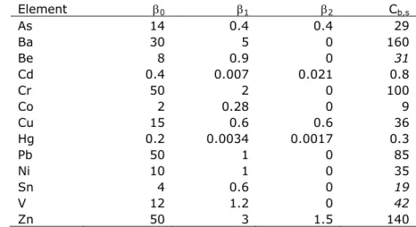
Table 3.1: Model parameters (see eq. 3,2) and Cb,s for the current soil type correction. Element 0 1 2 Cb,s As 14 0.4 0.4 29 Ba 30 5 0 160 Be 8 0.9 0 31 Cd 0.4 0.007 0.021 0.8 Cr 50 2 0 100 Co 2 0.28 0 9 Cu 15 0.6 0.6 36 Hg 0.2 0.0034 0.0017 0.3 Pb 50 1 0 85 Ni 10 1 0 35 Sn 4 0.6 0 19 V 12 1.2 0 42 Zn 50 3 1.5 140

The background value for standard soil (Cb,s) with 25 wt-% clay and 10 wt-% organic matter is thus given as

(3.2)

C





 25

10

Where Cb,s is the background concentration in standard soil. Model parameters for equation 3.2 are given in Table 3.1.

Normative values, e.g. from the Dutch Soil Quality Decree (VROM, 2007), are expressed as concentrations in standard soil (i.e. 25 wt-% clay and 10wt-% organic matter). To assess if soil concentrations measured in the field comply to a normative value, either the normative value should be expressed as a soil type specific value (i.e. left bar in Figure 3.1) or the measured soil concentration should be expressed as concentration in standard soil (i.e. right bar in Figure 3.1). By decree the formula to relate standard soil concentrations with soil type specific concentrations is (Anonymous, 2007):

(3.3) 2 1 0 2 1 0 ,

_

₂₅

_

₁₀

_



















C

L

O

C

Where Cb,s is the concentration in standard soil and C the concentration in a specific soil, L and O are the clay and organic matter fractions for this specific soil.

Looking at Figure 3.1, the line A'B' depicts the correction of a legislative value (B') in standard soil into a soil type specific value (A'). It is immediately clear that the slope of the line differs from the slope of the model, i.e. line AB. Despite the use of the added risk approach, the current use of the STC does not only result in correction for the background concentration, but also the added part is implicitly corrected. This can be numerically demonstrated: let us assume that the organic matter content in the specific soil is 10 wt-%, with this choice we neglect the variability in organic matter; then let 102+0=k, thus:

(3.4)

k

L

k

L

C

C









25



Which can be rewritten as:

(3.5)

k

kC

k

C

L

C











25

25







Equation (3.5) can be regarded as a linear function in the form y=ax+b, with x as the independent variable and a and b respectively the slope and intercept of the line described by this function. This line is depicted in Figure 3.1 as line A’B’ and it is clear that both slope and intercept depend on the choice of Cb,s, hence each normative value has its own line A’B’ with a slope and intercept different from AB.

The implication is as follows: the line AB and equation (3.1) depict the variability of a natural background concentration in a geographical area, or for differences in lithology, which spatially varies. It is this variability for which the STC is used and the relation underlying the STC is derived as a regression model based on field data. However, from equation (3.3) to (3.5), it is clear that the current STC formula describes a model (A’B’) with a different slope and intercept than equation (3.1), hence a model which is not representative for the observed variation in the field. This defies the original purpose of the STC.

So, if a soil quality criterion, a normative value, is recalculated from a standard soil into a concentration for the specific soil, then both background concentration (Cb) and the MPA are normalized. The implicit normalization of the MPA has no explicit purpose. It will be shown in section 4.3 that the anthropogenic addition is independent of soil variability, so there is no need to correct the MPA for background variability.

Sometimes it is stated that the correction of the MPA can be considered as a implicit correction for bioavailability, but this is not proper reasoning since the underlying model, equation (3.3), does not include bioavailability. Even more, the underlying model for the background concentrations (see Figure 2.2) assumes no adverse concentration by definition.

In summary, the STC formula from equation (3.3) only reflects reality when the natural background concentration is used. Any other value for Cs,b leads to a numerical artefact, and as a result the explained variability does not reflect reality. For these other values of Cs,b, the formula can be improved.

3.2 Improvements

To understand the improvements, one must understand the building blocks of the use of a soil type correction within soil management and their function in the creation of soil quality guidelines.

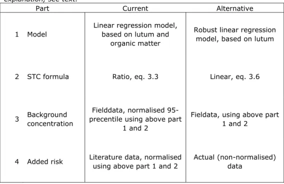
Table 3.2 shows the different parts, the building blocks, of the soil type correction. There are four parts:

1. The model is the statistical model, which describes the soil variability and gives the parameters (x) for the soil type correction formula. 2. The formula is the equation to normalise the soil concentration using the

3. In the added risk approach the background concentration and the added concentration are needed. The background concentration (Cb) is the third part. This background concentration can be derived by normalising field data using using the STC formula or it can be calculated directly from the model and STC formula.

4. The added risk can be normalised using the STC formula. But it is also possible to use actual data from literature, without normalisation. Table 3.2 contains options for each part. The options of the current STC are given and explained in section 3.1. In this section an alternative is proposed and its options are also given.

Figure 3.2 graphically represents the alternative from Table 3.2. In this scenario only the background concentration (Cb,, blue) is normalised. The MPA is kept constant. This reflects the option that the background concentration varies while the risk associated with the added concentration will not vary. This risk is regarded independent of soil type. This alternative neglects variability in availability as the concentration of many elements is only partial available for certain (bio)chemical reactions in soils. These partial concentrations include so called bio-available or potential (chemical) available concentrations

Table 3.2: The four parts for a soil type correction. For both the current STC and the proposed alternative STC the content of each part is given. For further explanation, see text.

Part Current Alternative

1 Model

Linear regression model, based on lutum and

organic matter

Robust linear regression model, based on lutum

2 STC formula Ratio, eq. 3.3 Linear, eq. 3.6

3 Background concentration

Fielddata, normalised 95-precentile using above part

1 and 2

Fieldata, using above part 1 and 2

4 Added risk Literature data, normalised using above part 1 and 2

Actual (non-normalised) data

Figure 3.2: scenario were only a correction is applied on the natural background variation.

From Figure 3.2 it is clear that a model for the variability in the background concentration is needed, like the current model as described in equation (3.1). Only the intercept of line A’B’ changes with changing the value for the MPA, in formula:

(3.6)

C









L

 C

Where L is the clay size fraction, Ca is the added concentration (see Figure 2.2) and 0,1 are respectively the intercept and the slope. This formula reflects the situation depicted in Figure 3.2, where 0.+Ca form the intercept of line A’B’. In the next chapters of this report the model parameters for the model in equation 3.6 will be derived and discussed. Using equation 3.6 as soil type correction formula for the background concentration, together with the derived parameters, it provides the data for the options in part 1 to 3 of the alternative STC in Table 3.2.

L=25%

L=12%

A’

B’

C

Cx, standardsoil

C

Cb, standardsoil

C

= C

Model C

, metal X

Clay fraction

C

(mg.kg

)

A

4

Geochemical baseline model for Dutch soils

In the previous chapter it was explained that the soil type correction (STC) is based on a model which predicts (natural) background concentrations in soil. This model was derived about 20 years ago. More recently, the Geochemical Atlas of the Netherlands was published (Mol et al., 2012) and based on the original work of Van der Veer (2006). This is a study into the geochemical composition of Dutch soils. One of the objectives of the study was to reduce variability as a result of sampling and analytical procedures. With this reduction subtle patterns in the geochemical composition of Dutch soils can be discerned, like spatial variability of natural trace element concentrations with the major soil composition.

While the first edition of the Geochemical Atlas aimed at presenting total concentrations (Van der Veer, 2006), as measured by X-ray Fluorescence (XRF) and HF-digested soil samples analysed with Inductive Coupled Plasma-Mass Spectrometry (ICP-MS), the latest edition also contained reactive concentrations (0.43 M HNO3 extracted soil samples analysed with ICP-MS and ICP-OES, Optical Emission Spectrometry) and available concentrations based on 0.01 M CaCl2 extractions of the soil samples. This means that the dataset of the Geochemical Atlas provides a nation wide overview of total, reactive and exchangeable concentrations of major and trace elements which gives

information about soil composition, soil reactivity and (bio)availability. By using this dataset, the derived models can be related to other soil processes than soil composition alone. For example relations with soil leaching or risks for the ecosystem.

From the data of the Geochemical Atlas a relation between soil composition and trace element concentrations is derived. This relation, a geochemical baseline model, was developed to estimate the natural background concentration in a diffusely polluted soil (Spijker et al., 2012). This model is applicable for the whole area of the Netherlands. Since the natural background concentration is the basis of the normalization of soil concentrations (like the STC) and because the baseline model describes the spatial variability of the natural background concentration, it was chosen to use this model as an alternative for the STC. In the next sections we will explain some details about this geochemical baseline model and how this model can be used to 1) obtain the natural concentrations as needed the for the scenario in Figure 3.2 and 2) to confirm the added risk approach mentioned in chapter 2.

4.1 Aim of the baseline model

The aim of the baseline model is to describe the natural variability between the bulk geochemistry and trace elements in a simple statistical manner. Like the relations currently used in the STC. However, the model is not based on clay size fraction but on Al2O3. Some authors already pointed out that there is a close relation between trace elements and this bulk geochemistry. Spijker (2005) and Van Gaans et al. (2007) have shown that for the marine clayey soils in the South-West of the Netherlands a strong relation exists between trace element geochemistry and Al2O3 as measured by XRF. Spijker (2005) used a relation where the trace element content was expressed as function of Al2O3, using an ordinary least square linear regression model. Van der Veer (2006) showed that the same method of regression as used by Spijker (2005) applies to all major

soil types in the Netherlands. It is therefore that Al2O3 was chosen as predicting variable for the baseline model.

Organic matter is not part of the model. Van der Veer (2006) showed that organic matter content is partly related to mineral organoclay aggregates in soil. This means that a part of the variability of trace elements with organic matter is explained by the variability in clay content, which is covered by the variability in Al2O3. Spijker et al. (2008, 2012) showed that adding organic matter as variable to the baseline model does not improve the estimation of the natural

background concentration, hence organic matter was excluded from the model. 4.2 Regression model

The baseline model is, like the STC, a regression model using Al2O3 as predicting variable. This regression model is described in Spijker et al., (2012). It is a robust regression model using the Least Quantiles of Squares (LQS) algorithm (Leroy and Rousseeuw, 1986) Based on the results of Spijker (2005) and Van der Veer (2006), the following linear model was used for the LQS regression: (4.1)

C









C





Where C is the estimated total trace element concentration, using CAl expressed as Al2O3 in wt-%. The regression parameters 0,1 are calculated using the LQS method mentioned above. The regression error ε gives the deviation of the residuals, which represents the variation not explained by the variability in Al content.

According to Leroy and Rousseeuw (1986) the linear interval of 2.5ε compares to the range of the normal distributed residuals. Since the LQS method does not assume normality of the data, no values determining significance of the

regression are derived.

Spijker et al. (2012) showed that the baseline model gives a good prediction of the variability in natural background concentrations. These baseline models were created for As, Ba, Be, Cd, Cr, Cu, Pb, V, Zn, Ni, Sb, Sn and are shown in Figure 4.1. From this figure the good prediction of the baselines is clear. For each distinct soil lithology in the Netherlands (peat, sand, fluvial clays, and marine clays) a model was created and also a generic model for all soil types together. This generic model, the lines depicted in Figure 4.1, complies to the wish for a simple model to describe the Dutch soil geochemistry, and can be used as an alternative normalization procedure. From Figure 4.1 it is apparent that this generic model describes the soil variability very well, with Ba being an exception.

Figure 4.1: plots of each element (y-axis) against Al2O3 (x-axis).

Element concentrations are in mg/kg, Al2O3 concentrations is in wt-%. The black dots are sub soil concentrations. The lines denote the generic regression model, solid line is the LQS regression line, dashed lines are the regression error (2.5ε). From Spijker et al., 2012

From the study of Spijker et al. (2012) it was apparent that the covariability of trace elements with Al2O3 in sandy soils (i.e. soils with low Al2O3) was far less than the covariability in clayey and peaty soils (see Figure 4.1). Although the generic baseline model described the overall variation very well, if one is interested in trace element concentrations in sandy soils, a sandy soil specific baseline model seems more appropriate. Geochemical baseline models for specific soil lithologies (e.g. sand, peat and clay) are available from Spijker et al.

(2012) but deriving a lithology specific STC model is beyond the scope of this study.

4.3 Confirmation of added risk approach

Using these baseline models the estimated concentration can be compared with the actual measured concentration; this gives the enrichment of elements compared to the baseline. Based on the ratio between estimated baseline concentrations and enrichment, the elements Cd, Pb, Sb, Zn and Cu are in general considered as enriched.

Figure 4.2 gives four examples of the baseline models of Cd, Cu, Pb and Zn (Spijker et al., 2011.). In the left part of the figure it can be seen that the top soil concentrations (black circles) are enriched compared to the sub soil concentrations (green crosses). Considering that the baseline model gives the natural background concentration, Cb within the added risk approach (see Figure 2.2), the enrichment then compares with the soil concentrations associated with risk. An assumption in the added risk approach is that this added fraction, the enrichment, is fully reactive while the background is inert. In the right part of Figure 4.2 the relation between reactivity (i.e. potential

availability) and enrichment is depicted. The 1:1 line is shown for comparison. From the figure it is apparent that the reactivity of these four metals is indeed comparable with the enrichment. This agrees with the assumption behind the added risk approach, see Figure 2.2. Hence, the principles behind the baseline model are suitable to predict the Cb.

Remarkably, organic matter is not part of the geochemical baseline model. As Spijker et al. (2008) and Spijker et al. (2012) explained, organic matter has limited value in the prediction of background concentrations. Adding organic matter to the model does not improve the prediction compared with a model without organic matter as variable.

Unfortunately the model of Spijker et al. (2012) is based on a relation of Al2O3 and total metal content, while the soil type correction and normative values are based on a regression model based on clay fraction, organic matter and

concentrations based on aqua regia digestions. Therefore, it can not directly be applied as replacement of the soil type correction, despite the fact that it is very suitable, see Mol and Spijker (2009) for a more detailed explanation. In the next chapters we will show how the model can be adapted so it can be used as an alternative for the STC.

Figure 4.2: (Left) Scatter plots depicting the way in which metal enrichments in the topsoil are estimated with a geochemical baseline model; green crosses subsoil sample metal concentrations; lines Al2O3 baseline models; black circles

topsoil sample metal concentrations. (Right) Linear relationships between reactive metal concentrations (0.43 M HNO3 extractable metal concentrations)

and enrichments (topsoil concentrations minus baseline-estimate

5

Method for an alternative model for background

concentrations.

One of the aims of this study is to obtain a practical and uncomplicated method to predict the Cb of a field sample. This Cb is the basis of the Added Risk Approach, discussed in chapter 2. The results presented in chapter 4, based on Spijker et al. (2012), indicate that it is indeed possible to get an estimate of the natural background.

An alternative method should be based on variables and measurements that are currently used in the field of soil management and sanitation, like the digestion of soil samples with aqua regia. Although there are state of the art techniques, like the geochemical baseline model of chapter 4, they are not widely used due to reasons related to laboratory infrastructure, safe working conditions, and costs. The alternative method or model should be simple and easy to apply to soil concentrations as well. This means for example that the method preferably should be relevant to the whole area of the Netherlands, instead of having several methods for different areas or lithologies.

With the geochemical baseline model it is possible to predict the background concentration of a field sample, likewise the current STC. However, this

geochemical baseline model is based on variables not used in common practice, i.e. total metal content and Al2O3. There are similarities though: the Al2O3 content is related to the clay content while the total metal content is related to the aqua regia digested concentrations used within the current practice.

Considering that 1) the geochemical baseline model is based on the total area of the Netherlands, 2) the sampling and analytical variance provide sufficient accuracy to describe the relations between major and trace elements, 3) the data can be related to not only composition but also to soil processes, and 4) the data is publicly available through the Dutch Geochemical Atlas, it was chosen to use this dataset for the alternative STC.

From literature and unpublished data it is possible to derive regression models of the relations between clay fraction and Al2O3. Also models can be derived for the relation of total metal content and aqua regia digested concentrations. By combining these models a model which relates clay content to trace element variability can be created. However, this means that by combining different regression models, the variability of some variables is explained solely based on these models rather then on data. From a statistical point of view this is

questionable, but from a pragmatic viewpoint it is sensible to base the new method on existing data and models. By combining these existing data and models one must be aware of the consequences. The resulting model should only be used, if used at all, as an engineering solution that just fits the current problem, and not as a scientific model to explain variability and significance. The resulting model will be validated against a fully independent dataset to see if it proper fits its purpose or that it results in a biased assessment.

This chapter shows the methodology behind an alternative STC model. This method is applied to the data of the Dutch Geochemical Atlas and the results are given in chapter 6.

5.1 Approach for using data from the Geochemical Atlas

As explained above, to derive a STC model from the geochemical baseline model, based on data from the Geochemical Atlas, three steps are necessary:

1. Create a model to expres Al2O3 as clay fraction (i.e. lutum).

2. Create a model to express total concentrations as concentrations based on aqua regia.

3. Combine both models to create a model in which the background concentration is expressed as function of clay fraction.

After creating the final model, the model should be validated to see of the model does explain the natural variability of trace element concentrations in a

satisfying way. In the next sections these steps will be discussed. 5.2 Relation between Al2O3 and lutum

Clay size fraction in the Netherlands is measured as ‘lutum’, the clay fraction with grain size <2 μm. Two methods are currently in use, one is the pipette method, the other is based on laser diffraction. Both methods are described in Buurman et al. (2001). Buurman et al. (2001) have noted that the methods are not comparable. Although measurements of the clay fraction in both methods are highly correlated (R2_{>0.95), the absolute clay fractions differ by a factor up} to 2. Both methods are also dependent on the exact laboratory procedure. To our knowledge there is no good dataset available, which relates lutum with Al2O3. For this study the data of Edelman (1984) and the National Soil Monitoring Network were available and contained both total Al concentrations and clay size fractions. However, they did not contain sufficient information about the method used for measuring lutum. Therefore the relation between Al2O3 and clay size fraction in these datasets were hard to interpret. As a result, it was chosen to select a relation of Al2O3 and clay size fraction from literature. In Spijker (2005) a relation is described between Al2O3 and clay size using the same method for Al2O3 as the Geochemical Atlas and a method applied in commercial laboratory, using pipettes, for the clay size fraction. The latter method reflects the common method as used in Dutch practice. This relation is given as:

(5.1) Clay = 4.76 Al2O3 -15.47

Equation (5.1) does not apply for sandy soils, which contain approximate 2 to 3 wt% Al2O3 (Mol et al., 2012). Using equation (5.1) the Al2O3 concentrations for other soils are expressed as wt-% clay (see section 6.1).

5.3 Relation between total concentration and aqua regia

Common practice requires that soil concentrations of metals and metalloids within the frame work of the Dutch Soil Quality Decree are expressed as

concentration after an aqua regia extraction, an extraction with a hot mixture of three parts hydrocholoro-acid and one part concentrated nitric acid. With this extraction only partial concentrations are obtained. The data of the Geochemical Atlas was analysed using so called total methods, either using X-Ray

fluorescence or digestion in a hydrofluro-acid mixture. These latter concentrations are generally higher than the aqua regia extracted

concentrations. Hence, for the alternative STC the total concentrations of the atlas should be expressed as concentrations measureded by aqua regia extractions.

We selected unpublished data from the Dutch Soil Monitoring Network in which samples of Dutch soil were analysed using both total and aqua regia methods. The total method uses the same analytical procedure as for the data from the Geochemical Atlas. The aqua regia method is an in house method of the laboratory of the Dutch Geological Survey/TNO, comparable with commercial methods.

For each element, a robust LQS regression model was created were the aqua regia concentration (Car) was expressed as function of the total

concentration(Ct), according to: (5.2)

C









C





In equation (5.2) 0,1 are respectively the intercept and slope of the regression and  is the regression error. The statistical method, the LQS regression, was the same as for the geochemical baseline (see chapter 4).

Using the model in equation (5.2) the total concentrations of the Geochemical Atlas are expressed as aqua regia concentrations (see chapter 6.2).

5.4 Relation between lutum and trace element concentrations In the two steps described above the data of the Geochemical Atlas are expressed in concentrations which are comparable with concentrations as demanded in de Soil Quality Decree. Metals and metalloids are expressed as concentrations measured using an aqua regia extraction, and Al2O3 is expressed as clay size fraction. These data are now suitable to create a relation of clay size with trace element concentrations. This is likewise the estimation of the

background concentration in the current STC (see chapter 2).

Again a regression model was created based on the sub soil data of the

Geochemical Atlas, using the same method and LQS regression model as Spijker (2012). Clay size (lutum) was used as independent variable. However, as discussed in section 4.2 the covariation of Al2O3 with trace elements is low in sandy soils and, discussed in section 5.2, there is no suitable model available for the relation between Al2O3 and lutum for small lutum values (<5 wt-%).

Therefore the model is assumed to be variable for clayey and peaty soils, and constant for sandy soils. In the model soils with a clay size fraction lower than 5 wt-% are defined as sandy soils. This results in the following formula:

(5.3)































5

5

.

2

5

5

5

.

2

L

L

L

C













Where C is the concentration of the metal or metalloid and L is the clay size fraction. The parameters 0,1 are respectively the intercept and slope, and  is the regression error. By using 2.5ε the upper limit of the error interval is chosen and 90% of the values fall below this level (see Leroy and Rousseeuw 1986) 5.5 Model error

Ideally, the fitted model of equation (5.3) is validated against an independent dataset. Unfortunately, for this study there are no datasets available which use the same method for measuring trace element concentrations and grain size as used with the datasets for which the above model was derived. To get an

impression of the residual variability of the model compared with field data, three datasets were selected for comparison.

The first dataset is the dataset of the inventory study of Brus et al. (2009), this is the so called ‘AW2000’ dataset. This dataset was chosen for two reasons. First, these data are based on metal and metalloid concentrations measured after an aqua regia extraction using commercial available methods. Clay size fractions were also measured using commercial methods. Secondly, legislative threshold values of the Dutch Soil Quality Decree are based on this dataset. The second study is the dataset of the Dutch Soil Monitoring Network, this dataset has a slightly different analytical procedure based on extraction with fleischman acid (a mixture of concentrated sulphuric and nitric acid) and clay size fraction using the pipette method. This dataset is, like the dataset of Brus et al. (2009), based on a nationwide sampling and in comparison with AW2000 gives an indication of analytical variability.

Additionally an unpublished dataset from the area of Zuid-Holland is used. This dataset was chosen because it was sampled from peaty soils, containing high organic matter. This dataset is more representative for soils with high organic matter than the other two datasets.

All three datasets contain trace element concentrations and grain size fractions. However, the methodology for measuring trace elements concentrations can differ between the studies.

In chapter 6 the alternative STC is compared with the field data in two ways. First the trace element concentrations are plotted against the clay size fraction. This gives an indication of the covariability between clay size fractions and trace elements as obtained by the different analytical techniques. Second the natural trace element background concentration is estimated by 1) the alternative STC (see equation (5.3)) and 2) the original STC (see equation (3.5)) and plotted against the observed concentrations. Data used for this step are the sub soil concentrations from the inventory study of Brus et al. (2009). This gives an indication of how the alternative STC perform in comparison with the original STC. Since the intercept of the regression model of the original STC was increased to an upper level, the 90-percentile, of the residual variance of the regression, it is expected that in comparison with observed values the predicted values are an overestimation. The covariance between observed and predicted however, should be comparable.

Although this method is not a validation common in statistical analysis, it gives an impression of the fit of the model for the chosen datasets.

5.6 Consequences

The current normative values form metals and metalloids, as defined in the Soil Quality Decree (VROM, 2007), are based on the 95-percentile from the

inventory study (Brus et al., 2009) together with an ecological risk level, as explained in chapter 2. These 95-percentiles are derived after normalising the measured top soil concentrations in the field using the current STC. Again, a change in model of the STC means that the data of the inventory study also should be re-evaluated. Luckily, normalising the data of the inventory study using the alternative STC and calculating the 95-percentile, using the same weights as Brus et al. (2009), can be easily performed. So, to obtain an

impression of the consequences when the alternative STC model parameters are used, the resulting weighted 95-percentiles are calculated based on normalised data. For this normalisation the following formula is used (see equation (3.3)):

(5.4)

C

 C

C

C

Where Cs is the normalised concentration, Cf is the measured concentration, Cb is the concentration calculated with equation (5.2) using L=25 wt-%. Cb,f is the concentration calculated with the same equation (5.2) but then with L being the measured grain size fraction of the field sample.

The method of equation (5.4) is equal to the current formula of the STC (see equation (3.3)) and shows what happens if the current STC model parameters are exchanged by the alternative parameters. This ignores the fact the 95-percentile is a different property than the natural background concentration and is subject to the problem presented in equation (3.5). Both current and the alternative STC of equation (5.4) are, senso stricto, not representative for the soil concentrations in the range of the 95-percentile. However, it will give an indication of the consequences.

6

Results and discussion of the alternative model

6.1 Relation between lutum and Al2O3

For the relation between the clay size fraction (‘lutum’, grain size <2m) a fixed relation was used (see equation 5.1). This relation is plotted in Figure 6.1 together with data from two independent datasets as comparison. The first dataset is the one from Edelman (1984), where lutum was measured with the pipette method and Al using Instrumental Neutron Activation Analyses (INAA). The other dataset is unpublished data from the National Soil Monitoring Network (Landelijk Meetnet Bodem , LMB). In this dataset lutum was measured using laser diffraction and Al was determined using X-Ray Fluorescence.

In Figure 6.1 the line of the used relation of lutum vs. Al seems to fit the Edelman data better then the LMB data, the latter showing lower values for lutum (or higher values for Al2O3) and less variance in Al2O3.

Figure 6.1: The relation of Al2O3 with lutum (line) together depicted with data

from two independet datasets (Edelman and LMB). For explanation, see text.

Figure 6.1 also shows no apparent relation between Al2O3 and clay size for clay size fractions lower than 5 wt-%. This confirms the choice not to derive a alternative STC for soil with clay size fractions below 5 wt-%.

6.2 Relation between total concentration and aqua regia

From the unpublished dataset of the National Soil Monitoring Network 22 data points were selected where each element was both analysed using aqua regia and total methods. The relation between total and aqua regia method is depicted in Figure 6.2. The regression parameters are given in Table 6.1.

Opposite page: Figure 6.2: Relation between total concentrations (x-axis) and aqua regia extracted concentrations (y-axis) for 15 trace elements. The dashed lines indicate the 1:1 line, the solid line is the regression model, dotted lines indicate the 2.5ε range.

Table 6.1 Regression parameter (0,1), regression error () and robust

correlation coefficient (r) of the relation between total metal concentrations and aqua regia extraction (see equation (5.2)).

Element 1 0  r As 0.81 1.15 0.57 0.98 Ba 0.50 -84.0 12 0.52 Be 1.0 -0.350 0.052 0.99 Cd 1.1 -0.107 0.018 0.74 Cr 1.4 -56.0 2.9 0.99 Cu 1.00 -0.00167 0.11 0.91 Pb 1.2 -6.52 0.93 0.98 V 0.85 -2.25 1.6 0.99 Zn 0.98 13.1 1.4 1.00 Mo 1.0 -0.115 0.038 0.97 Ni 0.92 0.486 0.85 0.98 Sb 0.47 0.00730 0.028 0.82 Se 0.89 -0.268 0.037 0.97 Sn 0.78 -0.260 0.12 0.84 Tl 0.96 -0.081 0.046 0.82

Figure 6.2 shows in general a good relation between the aqua regia and the total methods The robust correlation coefficient confirms these good relations, in general r>0.90. Exceptions are Ba, Cd, Sb, Sn and Tl. For Ba r=0.52, for Cd r=0.74 and for Sb, Sn and Tl r>0.80.

For Ba it is generally known that the total concentration of this element can not be properly measured using an aqua regia extraction. For Cd, Sn Tl and Sb it is known that the reproducibility is relatively large, i.e. less accurate, for both the aqua regia extraction and the HF digestion (see Mol and Spijker, 2009, for a detailed discussion about the analytical methods).

6.3 Relation between lutum and aqua regia

In the above two sections regression models were derived which express aqua regia concentrations and grain size fraction as function of total concentrations and Al2O3 respectively. With these regression models the metal and metalloid concentrations of the Dutch Geochemical Atlas were recalculated as data expressed in aqua regia concentrations and Al2O3 was expressed as lutum. The trace element concentration can be expressed as function of lutum using a regression model cf. equation (5.3). These results are shown in Figure 6.3 and Table 6.2.

Table 6.2: constants for the STC regression, including regression error, see equation (5.3). R is the robust correlation coefficient based on the Minimum Volume Ellipsiod. The range of predicted concentrations is given in Table 6.3.

Element 0 1 error r As 3.72 0.207 2.93 0.81 Ba 36.6 0.779 17.21 0.60 Be 0.142 0.0439 0.137 0.96 Cd -0.0390 0.00317 0.0607 0.65 Cr -9.05 2.10 7.30 0.97 Cu 0.679 0.256 3.21 0.88 Pb 2.45 0.417 2.52 0.94 V 9.59 1.80 6.64 0.96 Zn 17.66 1.99 6.70 0.97 Mo -0.00683 0.0146 0.225 0.69 Ni 2.363 0.773 3.01 0.97 Sb 0.149 0.00347 0.0349 0.84 Se 0.099 0.0214 0.226 0.77 Sn 0.145 0.0442 0.133 0.98 Tl 0.0931 0.0108 0.0454 0.95

Table 6.2 shows that the correlation between the clay size fraction and the trace element concentration is good (R>0.9). The elements As, Cu, Sb, Se have somewhat lesser correlation coefficients (0.77<R<0.88). Barium, Cd, and Mo have a R of respectively 0.60, 0.65 and 0.69. For Ba it is already stated that this element is difficult to analyse using aqua regia. For Cd and Mo relatively large values for duplicate precision are reported (Van der Veer, 2006).

In Figure 6.3 the model prediction is shown graphically. The robustness of the model is clear when, for example, if one looks at Cd and Cu. Higher, more outlieing values, have minor impact on the direction of the regression line. Barium clearly shows that a generic model is in some cases not favourable. Figure 6.3 shows that for Ba the generic model follows the variability in clayey soils which is distinctively different from sandy soils (i.e. the grey dots).

Figure 6.3:Regression models of lutum, recalculated from Al2O3, and trace

element concentration, recalculated from total concentrations. Regression parameters are given in Table 6.3.