Probabilistic risk assessment for new and existing chemicals: Example calculations | RIVM

Hele tekst

(1)research for man and environment. RIJKSINSTITUUT VOOR VOLKSGEZONDHEID EN MILIEU NATIONAL INSTITUTE OF PUBLIC HEALTH AND THE ENVIRONMENT. RIVM report 679102 049 Probabilistic risk assessment for new and existing chemicals: Sample calculations T. Jager, H.A. den Hollander, G.B. Janssen, P. van der Poel, M.G.J. Rikken, T.G. Vermeire January 2000. This investigation has been performed by order and for the account of the Directorate-General for Environmental Protection, Directorate of Chemicals, External Safety and Radiation Protection of the Ministry of Housing, Spatial planning and the Environment, within the framework of project 679102 "Risk assessment methodology".. RIVM, P.O. Box 1, 3720 BA Bilthoven, telephone: 31 - 30 - 274 91 11; telefax: 31 - 30 - 274 29 71.

(2) page 2 of 60. RIVM report 679102 049. Abstract In the risk assessment methods for new and existing chemicals in the EU, "risk" is characterised by the deterministic quotient of exposure and effects (PEC/PNEC or Margin of Safety). From a scientific viewpoint, the uncertainty in the risk quotient should be accounted for explicitly in the decision making. The advantages and disadvantages of probabilistic risk assessment in this legal framework have been extensively discussed in earlier work. To demonstrate the benefits of a probabilistic risk framework, sample assessments for two substances, an existing chemical (dibutylphthalate, DBP) and a new chemical notification (anonymous), are presented in this report. The two examples worked out here show a probabilistic risk framework to be feasible with relatively little extra effort; such a framework also provides more relevant information. The deterministic risk quotients turned out to be worst cases at generally higher than the 95th percentile of the probability distributions. Sensitivity analysis has proven to be a powerful tool in identifying the main sources of uncertainty and thus will be effective for efficient further testing..

(3) RIVM report 679102 049. page 3 of 60. Contents Summary .................................................................................................................... 4 Samenvatting ............................................................................................................. 6 1.. Introduction ................................................................................................................. 8. 2.. Method for uncertainty analysis ................................................................................. 9. 3.. Alternative scenarios ................................................................................................. 11. 4.. Interpretation of probability distributions ............................................................... 12. 5.. Probabilistic assessment of DBP ................................................................................ 14 5.1 Introduction to DBP ................................................................................................ 14 5.2 Conclusions of the dossier and EUSES .................................................................... 14 5.3 Probabilistic risk assessment ................................................................................... 15 5.4 Conclusions for DBP ............................................................................................... 21 5.5 New data for DBP .................................................................................................... 21 5.6 Alternative scenarios for DBP (new data) ................................................................ 26 5.7 Conclusions new data .............................................................................................. 30. 6.. Probabilistic assessment of a new chemical .............................................................. 32 6.1 Introduction to the new chemical ............................................................................. 32 6.2 Conclusions of the dossier and EUSES .................................................................... 32 6.3 Probabilistic risk assessment ................................................................................... 33 6.4 Conclusions for the new chemical ............................................................................ 37. 7.. Conclusions ................................................................................................................ 38. References .......................................................................................................................... 41 Appendix 1 Mailing list ..................................................................................................... 42 Appendix 2 Parameter distributions ................................................................................. 43 2.1 Default distributions ................................................................................................ 43 2.2 Release estimation ................................................................................................... 45 2.3 Partition coefficients, degradation, BCFs and environmental exposure ................... 54 2.4 Ecological effects assessment ................................................................................... 55 2.5 Human health effects assessment ............................................................................. 57 2.6 Parameters for Spain and Finland ........................................................................... 60.

(4) page 4 of 60. RIVM report 679102 049. Summary Risk assessment of new and existing chemicals in the EU is performed according to a harmonised methodology, laid down in technical guidance documents (TGDs), and implemented in the decision support system EUSES. In this framework, “risk” is characterised by the deterministic quotient of exposure and effects (PEC/PNEC or Margin of Safety). As the data basis of these risk assessments is usually narrow, a considerable degree of uncertainty accompanies these calculations. From a scientific viewpoint, this uncertainty should be accounted for explicitly in the decision making. The advantages and disadvantages of probabilistic risk assessment in this legal framework have been extensively discussed in earlier work. Nevertheless, the people involved in risk assessment and risk management in the EU are hesitant to support these developments. To demonstrate the benefits of a probabilistic risk framework, sample assessments for two substances are presented in this report: an existing chemical (dibutylphthalate, DBP) and a new chemical notification (anonymous). In uncertainty analysis, the choice for a certain parameter distribution is quite important. As this is not a trivial matter, there is a clear need for agreed default parameter distributions for the purpose of risk assessment. For this study, probability distributions were assigned to “chemical-specific” parameters (e.g. emissions, partition coefficients) and not to “environmental” or “scenario-dependent” parameters (e.g. organic matter content in soil, wind speed, dilution factors in surface water). The reason for the omission of this source of uncertainty is that it is virtually impossible to transparently capture this variability in a probability distribution. For these calculations, it was judged more appropriate to tackle this source by using alternative plausible scenarios (e.g. a real worst case and a best case) to provide a feel for the impact of these uncertainties. The examples demonstrate that environmental variability may well dominate the total uncertainty in a risk assessment and should be explicitly addressed. This is especially true for the local aquatic system, caused by the large range of the dilution factor in surface water. It should, however, be noted that the models in the TGD do not always allow for alternative scenarios. The flexibility of the models should therefore be considered in the update of the TGD. The worked-out examples for DBP and the new chemical demonstrate that a probabilistic risk assessment is feasible with relatively little extra effort and provides more relevant information. The width of the risk quotient distribution (5th-95th percentile) varied between chemicals and endpoints from 1 to 5 orders of magnitude in extreme cases (usually, less than 3 orders). The deterministic risk quotient of EUSES turned out to be worst case (generally higher than the 95th percentile) although this is not necessarily a general rule for all chemicals and depends on our particular choices for input distributions. The use of a sensitivity analysis to identify the main sources of uncertainty proves to be a powerful tool to decide where further testing is most efficient. The distributions assigned to the assessment factors (derivation of the PNEC) proved to dominate the total uncertainty in the risk assessment of these sample chemicals. Uncertainties in the release estimates come second. The effects assessment remains a critical stage when we want a probabilistic risk framework that is scientifically justifiable; the uncertainties in this part need to be addressed but the concept of the PNEC forms a problem in itself. A PNEC is not a measure of ecosystem damage but a conservative trigger value. Furthermore, the exceedance of the PNEC is not a risk level, in fact, the absolute value of the PEC/PNEC ratio cannot be interpreted as the shape of the (theoretical) relationship between exposure level and ecosystem damage is unknown..

(5) RIVM report 679102 049. page 5 of 60. Risk assessment is a process where we use limited information to predict the potential of chemicals to cause some toxic effect on different kinds of biotic endpoints. Large uncertainties are an inherent part of this process that we have to deal with. If we want a more realistic and defensible risk assessment, we have to get rid of protective and worst-case thinking in the risk assessment itself. Risk assessment should be as scientific and realistic as possible and that implies that we must admit what we don’t know. Attempting to quantify uncertainties is a good step in that direction; we believe that even a rough quantification of uncertainties is better than giving a false sense of accuracy. Further work is necessary in the following areas: • Guidelines how to perform an uncertainty analysis. • Agreed default distributions for basic parameters, especially in the release estimation and effects assessment. • Serious revision of the effects assessment (attempt to quantify real impacts). • Choice of alternative scenarios or other ways to address variability. • Thoughts on how to implement uncertainty analysis in risk characterisation and in risk management in the (near) future (e.g. which percentiles to take). It is the intention to present this report as contribution to the update programme of the EUTechnical Guidance Documents in 2000..

(6) page 6 of 60. RIVM report 679102 049. Samenvatting De risicobeoordeling van nieuwe en bestaande stoffen wordt in de EU gedaan met een geharmoniseerde methodologie, vastgelegd in technische leidraden (TGDs) en geïmplementeerd in het beslissings-ondersteunende systeem EUSES. In dit kader wordt “risico” gekarakteriseerd door het deterministische quotiënt van blootstelling en effect (PEC/PNEC of een Margin Of Safety). Een aanzienlijke hoeveelheid onzekerheid begeleidt deze berekeningen omdat de databasis gewoonlijk beperkt is. Vanuit wetenschappelijk oogpunt is het aan te bevelen deze onzekerheid expliciet in de besluitvorming mee te nemen. De vooren nadelen van een probabilistische risicobeoordeling in dit wettelijke kader zijn in eerder werk uitgebreid besproken. Desondanks zijn de mensen betrokken in risicobeoordeling en risicomanagement weinig enthousiast over deze ontwikkelingen. In dit rapport zijn daarom twee voorbeeldstoffen doorgerekend om de voordelen van een probabilistisch risicokader te demonstreren: een bestaande stof (dibutylftalaat, DBP) en een notificatie van een nieuwe stof. De keuze voor parameterverdelingen is enorm belangrijk in onzekerheidsanalyse. Omdat dit geen triviale zaak is, is er een duidelijke behoefte aan geaccepteerde defaultverdelingen voor risicobeoordeling. Voor deze studie is de keuze gemaakt om verdelingen toe te wijzen aan “stof-specifieke” parameters (bijv. emissies, partitiecoëfficiënten) en niet aan “milieu” of “scenario-afhankelijke” parameters (bijv. organisch stofgehalte van de bodem, windsnelheid, verdunningsfactoren in oppervlaktewater). De reden voor deze omissie is dat deze bron van onzekerheid vrijwel onmogelijk op een transparante manier in een verdeling kan worden beschreven. Voor deze berekeningen is gekozen voor het laten zien van alternatieve plausibele scenario’s (bijv. een echte worst-case en een best-case) om een idee te krijgen van de invloed van deze onzekerheden. De voorbeeldberekeningen tonen aan dat natuurlijke variabiliteit heel goed de totale onzekerheid kan domineren en dus meegenomen moet worden. Dit is speciaal het geval voor het lokale aquatische systeem door de grote spreiding in de verdunning in oppervlaktewater. De modellen in de TGD laten het gebruik van alternatieve scenario’s echter niet altijd toe. De flexibiliteit van de modellen moet dus worden meegenomen in de update van de TGD. De uitgewerkte voorbeelden voor DBP en de nieuwe stof laten zien dat een probabilistische risicobeoordeling met weinig extra moeite haalbaar is en meer relevante informatie geeft. De breedte van de risicoverdeling (5e-95e percentiel) verschilt tussen stoffen van 1 tot 5 ordegroottes in extreme gevallen (meestal minder dan 3 ordes). Het deterministische risicoquotiënt van EUSES blijkt behoorlijk worst-case te zijn (i.h.a. groter dan het 95e percentiel) hoewel dit afhangt van onze specifieke keuze van invoerverdelingen. Het gebruik van gevoeligheidsanalyse voor het identificeren van de belangrijkste bronnen van onzekerheid is een krachtig instrument om te besluiten waar verder testen het meest efficiënt is. De verdelingen toegewezen aan de “assessment” factoren (in de afleiding van de PNEC) blijken de totale onzekerheid te domineren in de risicoschatting van deze voorbeeldstoffen. Onzekerheden in de emissieschatting komen op de tweede plaats. De effectbeoordeling blijft een kritische stap als we een wetenschappelijk verantwoord probabilistisch risicokader willen; niet alleen moeten de onzekerheden worden gekwantificeerd, het concept van de PNEC vormt zelf een probleem. Een PNEC is slechts een conservatieve limietwaarde, geen maat voor schade aan ecosystemen. Verder is de mate van overschrijding van de PNEC geen risicomaat; in feite kan de absolute waarde van het PEC/PNEC quotiënt niet geïnterpreteerd worden omdat de vorm van de (theoretische) relatie tussen blootstelling en ecosysteemschade.

(7) RIVM report 679102 049. page 7 of 60. onbekend is. Risicobeoordeling is een proces waarbij we beperkte informatie gebruiken om de potentie van een stof in te schatten om toxische effecten te bewerkstelligen op allerlei organismen. Grote onzekerheden zijn een inherent deel van dit proces waar we rekening mee moeten houden. Als we een meer realistische en verdedigbare risicobeoordeling willen moeten we af van het beschermende worst-case denken in de risicobeoordeling zelf. Risicobeoordeling moet zo wetenschappelijk en realistisch mogelijk zijn en dat houdt in dat we moeten toegeven wat we niet weten. Volgens ons is zelfs een ruwe inschatting van de onzekerheid beter dan het geven van een vals gevoel van nauwkeurigheid. Proberen de onzekerheden te kwantificeren is een stap in de goede richting, maar vervolgonderzoek is nodig op de volgende gebieden: • Richtlijnen hoe onzekerheidsanalyse uit te voeren. • Geaccepteerde defaultverdelingen voor basale parameters, speciaal voor de emissieschattingen en de effectbeoordeling. • Ingrijpende revisie van de effectbeoordeling (pogen echte schade te kwantificeren). • Keuze voor alternatieve scenario’s (of andere manier om variabiliteit te behandelen). • Overweging hoe onzekerheidsanalyse kan worden geimplementeerd in de risicokarakterisering en risicomanagament in de (nabije) toekomst (bijv. welke percentielen te nemen). Het is de bedoeling om dit rapport in te brengen bij de revisie van de EU-technische richtlijnen (TGD) in 2000..

(8) page 8 of 60. 1.. RIVM report 679102 049. Introduction. Risk assessment of new and existing chemicals in the EU is performed according to a harmonised methodology which is laid down in so-called technical guidance documents (TGDs) (EC, 1996b). These TGDs are implemented in the decision support system EUSES (EC, 1996a). In this framework, it is agreed to characterise the level of “risk” by means of the deterministic quotient of exposure and effects (PEC/PNEC or Margin of Safety). As the data basis of these risk assessments is usually narrow, a considerable degree of uncertainty accompanies these calculations. From a scientific viewpoint, this uncertainty should be accounted for explicitly in the decision making. The advantages and disadvantages of probabilistic risk assessment in this legal framework have been extensively discussed (Slob & De Nijs, 1989; Jager & Slob, 1995; Jager, 1995; Jager et al., 1997) Nevertheless, the people involved in risk assessment and risk management in the EU are hesitant to support these developments. A series of interviews was conducted with ten representatives from Member States and chemical industry to learn about their viewpoints on uncertainty analysis and probabilistic risk assessment (Jager, 1998). These interviews were especially important to investigate whether a probabilistic framework is feasible and what types of further studies are necessary in this respect. Summarising, there seemed to be a guarded interest in uncertainty analysis among most of the people interviewed although it does not receive high priority at this moment. These interviews made clear that there is a gap between the scientist and the risk managers. In the scientific community, it is broadly accepted a necessity to provide confidence intervals when presenting secondary data. As a logical consequence, uncertainty analysis is broadly accepted as a necessity when presenting model results in a scientific manner. The risk manager, however, has to deal with the legal aspects and a decision must be reached within a certain time constraint. A series of probability distributions, although very scientific, does not seem to be an obvious help in this process. The best way to proceed with the work on uncertainty analysis is to try to bring together these two fields: it must be demonstrated how risk management can benefit from the extra work needed in performing and understanding probabilities. In our opinion, the best way to demonstrate this is by performing a few probabilistic risk assessments as examples and compare the results to the current TGD approach. At this moment, it is clear from the interviews that the uncertainty analysis must be kept as simple and transparent as possible to allow interpretation by non-statisticians. The first chapters of this report expand on the introduction by giving the framework for the uncertainty analysis (Chapter 2), discussing the use of alternative scenarios to tackle environmental variability (Chapter 3), and a short explanation on probability distributions (Chapter 4). Further in the report, sample risk assessments for two substances are presented. The first is dibutylphthalate (DBP, Chapter 5), an existing chemical for which a draft risk assessment has been prepared by the Netherlands in the existing chemicals programme of the EU. The second is a new chemical notification (name withheld, Chapter 6). The difference between the two data sets is large: for DBP, a large and evaluated data set is available whereas for the new chemical the data set is limited to the EU base set. This also means that the uncertainty in the final model results can be different. As much as possible, the parameter distributions were based on the data available for the compound, in other cases, general rules had to be used (Jager et al., 1997). Finally, Chapter 7 gives the general conclusions. It is the intention to present this report as contribution to the update programme of the EUTechnical Guidance Documents in 2000..

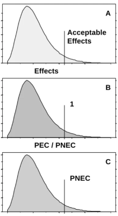
(9) RIVM report 679102 049. 2.. page 9 of 60. Method for uncertainty analysis. Before an uncertainty analysis can be done a choice must be made which uncertainties to represent in the analysis and in what way (the underlying assumptions). This is a crucial step as the interpretation of the resulting probabilistic risk measure will depend on it. For the purpose of these calculations, probability distributions were assigned to “chemical-specific” parameters (e.g. emissions, partition coefficients) and not to “environmental” or “scenario-dependent” parameters (e.g. organic matter content in soil, wind speed, dilution factors in surface water) (Jager et al., 1997). This distinction is not always straightforward; e.g. degradation rates depend on the chemical properties but also on the environmental temperature and bacterial populations. The use of “chemical-specific” uncertainties only, implies that environmental variability is not covered in the probability distributions. The reason for the omission of this source of uncertainty is that it is virtually impossible to capture this variability in a probability distribution in a transparent manner (Jager et al., 1997). Furthermore, several models in the TGD (and thus in EUSES) are not suited for including variability as they are tailored to a specific scenario (especially the local air model). Nevertheless, variability may be an important source of uncertainty. For these calculations, it was judged more appropriate to tackle this source by using alternative plausible scenarios (e.g. a real worst case and a best case) to provide a feel for the impact of these uncertainties (see Chapter 3). A source of uncertainty that is not addressed is the fundamental uncertainty in the model concepts (e.g. the assumption of well-mixed compartments in SimpleBox) and the choices for scenarios (e.g. exposure to air at 100 m from the source). It should be acknowledged that these uncertainties may well compromise the accuracy and precision of a risk assessment. From the interviews (Jager, 1998), it became clear that there is currently little support for quantifying Acceptable the uncertainties in the effects assessment. The Effects scientific understanding of this part of the assessment was judged insufficient to warrant even a limited Effects quantification. The uncertainties in the effects assessment may, however, well dominate the B assessment (Jager et al., 1997). Therefore, two 1 options for probabilistic risk assessment will be worked out in this report: 1. Probabilistic risk estimate where the PEC is PEC / PNEC uncertain and the PNEC, or the NOAEL for C humans, fixed (option C in Figure 1). The result is a probability distribution of the PEC and “risk” PNEC is interpreted as the position of the curve in relation to the vertical line, the PNEC. 2. Probabilistic risk estimate where both PEC and PEC PNEC are uncertain (option B in Figure 1). Figure 1 Options for probabilistic risk Uncertainty in the PNEC results from uncertainty assessment. in the extrapolation steps (assessment factors). For humans, a comparable extrapolation to a probability density. A.

(10) page 10 of 60. RIVM report 679102 049. PNEL1 is performed. The result is a probability distribution of the PEC/PNEC quotient. “Risk” is interpreted as the position of the curve in relation to the vertical line PEC/PNEC=1. The effects assessment remains the critical stage when we want a probabilistic risk framework that is scientifically justifiable (Jager et al., 1997). The uncertainties in this part need to be addressed but the concept of the PNEC forms a problem in itself. A PNEC is not a measure of ecosystem damage but a conservative trigger value and the exceedance of the PNEC is not a risk level2. In fact, the absolute value of the PEC/PNEC ratio is difficult to interpret as the shape of the (theoretical) relationship between exposure level and ecosystem damage is unknown. A further limitation of the PNEC derivation is that only a part of the available toxicological information is used: only the lowest LC50 or NOEC. Unfortunately, our options to revise this stage are limited as the current state of knowledge is insufficient to estimate dose-response relationships of ecosystems or human populations with any degree of realism. The PAF approach as worked out earlier (option A in Figure 1) is a step in that direction but the support for this approach in the EU is currently limited. Further study in this area is however desirable. Uncertainty analysis was performed with the EUSES 1.00 equations programmed in Microsoft Excel™. This version was programmed for the purpose of testing the development of the official version of EUSES and includes the SimpleBox and SimpleTreat spreadsheets. Uncertainty analysis was performed using Crystal Ball™ version 4.0c, an add-in for Excel. Sampling was performed according to the Latin-Hypercube option, 2000 runs were sufficient to obtain smooth distributions. Crystal Ball contains a large gallery of distributions including lognormal, triangular and uniform (the assumed distributions for the sample calculations).. 1. Predicted No-Effect Level. This parameter is called a level as it is usually given as a dose (mg/kg BW/d) and not as a concentration. This approach differs from that in the TGD as in the TGD, no explicit extrapolation to a “safe” level is performed. 2 “Risk” is generally defined in the scientific community as an “impact” times the probability or frequency that this impact will actually occur. A clear example is the risk associated with flying in an airplane: risk is the expected number of casualties times the frequency of a plane crash (e.g. expressed as expected number of casualties per kilometer of air travel). In risk assessment we have two problems: probabilities are not routinely quantified and impacts are poorly defined (exceeding a PNEC says nothing about the impact on ecosystems)..

(11) RIVM report 679102 049. 3.. page 11 of 60. Alternative scenarios. For some parameters, the uncertainty caused by environmental variability is relatively straightforward to quantify. Examples are human consumption rates where distributions can be fitted on results of consumer surveys. Other sources of variability are much more difficult to capture in distributions. As an example, the fish for human consumption is caught in fresh surface water at the point of complete mixing of the effluent with the receiving water body. In reality, the fish moves around and fish may be caught at different distances from an STP. When considering one river it may be possible to capture this variability in an acceptable distribution but since most chemicals have more sources from which they enter the environment, the situation becomes complicated. One has to assume a distribution for the distance between the catch and the STP and a distribution for the probability that a fish is caught from a water where a certain source is located. Clearly, we enter in a web of interconnecting uncertainties which is extremely complicated to resolve. In the earlier calculations (Jager, 1995; Jager et al., 1997), we ignored this source of uncertainty entirely. For this report, we chose to handle variability by calculating alternative plausible scenarios for several endpoints. Although this is a poor way to represent the total influence of variability it provides some clues as to whether variability plays a role in the risk assessment. The following scenarios were selected: Surface water (local). Soil (local). Regional. STP discharging on a large river (dilution factor=10000) STP discharging on a small ditch (dilution factor=2) Releases to waste water discharged directly to surface water: in this case also a small ditch (dilution factor=2). High fraction organic carbon in soil (30%), high rain rate (4 times normal) Low fraction organic carbon in soil (0.1%), low rain rate (1/4 times normal) Normal organic carbon content but no sludge applied as fertiliser Spain vs. Finland (see Appendix 2.5). For the aquatic endpoints, we changed the dilution factor as most important scenario property: ranging from 2 (a small ditch) to 10,000 (a large river). Furthermore, a scenario is presented were the effluent is discharged directly into the surface water without STP. The connection percentage in the EU-Member States ranges from 45 to 100% which makes this scenario not unrealistic. Changing the organic carbon fraction in soil has several effects. A higher sorption coefficient in soil leads to lower degradation rates. This is incorporated in the TGD in the form of degradation classes; here, a linear relationship is assumed. A second effect is that terrestrial ecotoxicity data should be normalised to a standard soil. Here, we also assumed a linear relationship between the fraction organic carbon (Foc) and PNEC. The percentage of sludge used as fertiliser in agriculture ranges between 10 and 80%, therefore, also a scenario were no sludge is applied will be shown. Due to the way that the air module in EUSES is implemented, it was not possible to make different scenarios for deposition or atmospheric concentrations. For the regional scenarios, the differences in temperature between the model countries Spain and Finland were accounted for. This required the implementation of temperature dependencies of degradation rates and physico-chemical properties (Brandes et al., 1996) which is not part of EUSES..

(12) page 12 of 60. 4.. RIVM report 679102 049. Interpretation of probability distributions. Risk managers are not usually experienced statisticians, which may be a reason for the lack of enthusiasm for uncertainty analysis. The interpretation of distributions requires some knowledge of statistics and probability calculus. Therefore, we provide a short introduction in this chapter. Most people will be familiar with probability distributions for discrete stochastic variables. In the example of Figure 2: the sum of one throw with a pair of dice. The height of a bar means the probability of a certain outcome and the sum of all bars equals a probability of 1 or 100%. The probability of a sum of 2 is 1/36 (of the 36 possible outcomes, only one will yield a sum of 2; i.e. 1 and 1), the probability of 7 is highest: 6/36 or 1/6 (6 possible outcomes with a sum of 7). The right part of Figure 2 shows the same distribution in a cumulative form. Over the range of possible outcomes, the cumulative function rises from 0 to 1. At an x value of 8, the cumulative probability is 0.72. This means that when throwing a pair of dice, the probability of obtaining a sum lower or equal to 8 is 72%. The probability of getting a value higher than 8 is the reciproque value: 28%. 0.18. 1. 0.16 cumulative probability. 0.14 probability. 0.12 0.1 0.08 0.06 0.04. 0.8. 0.6. 0.4. 0.2. 0.02 0. 0 2. 3. 4. 5. 6. 7. 8. sum of dice. 9. 10. 11. 12. 0. 2. 4. 6. 8. 10. 12. 14. sum of dice. Figure 2 Probability distribution of a discrete variable (the sum of one throw with a pair of dice) shown left; the cumulative function shown on the right. For a continuous variable like our RCR1, the cumulative distribution (the right part of Figure 3) allows a similar interpretation although the cumulative is now a smooth curve. The probability function is, however, a different situation. Other than in the dice example, there are an infinite number of possible RCRs and the probability of any single RCR is infinitesimally small. A useful analogue for continuous functions is the probability density function (left part of Figure 3) which is the derivative (slope) of the cumulative function just as the probability distribution for the sum of the dice is defined by the “jumps” in the cumulative function in Figure 2. In contrast with probabilities, the probability density can take values larger than one but the area under the total curve is always one (or 100%). Probabilities are found by taking the area under a part of the density curve (as shown with the area in the left Figure 3).. 1. The term RCR (Risk Characterisation Ratio) is used in the context of the TGD and EUSES to cover all the quotients of exposure and effects, thus including both PEC/PNEC as well as the Margin Of Safety for human health assessments..

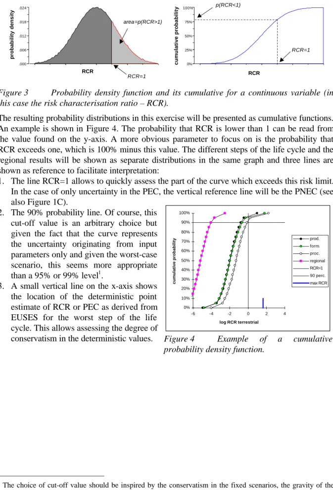
(13) page 13 of 60. probability density. .024. area=p(RCR>1). .018. .012. .006. .000. cumulative probability. RIVM report 679102 049. RCR. 100%. p(RCR<1). 75%. 50%. RCR=1. 25%. 0%. RCR. RCR=1. Figure 3 Probability density function and its cumulative for a continuous variable (in this case the risk characterisation ratio – RCR).. cumulative probability. The resulting probability distributions in this exercise will be presented as cumulative functions. An example is shown in Figure 4. The probability that RCR is lower than 1 can be read from the value found on the y-axis. A more obvious parameter to focus on is the probability that RCR exceeds one, which is 100% minus this value. The different steps of the life cycle and the regional results will be shown as separate distributions in the same graph and three lines are shown as reference to facilitate interpretation: 1. The line RCR=1 allows to quickly assess the part of the curve which exceeds this risk limit. In the case of only uncertainty in the PEC, the vertical reference line will be the PNEC (see also Figure 1C). 100% 2. The 90% probability line. Of course, this 90% cut-off value is an arbitrary choice but 80% given the fact that the curve represents prod. 70% the uncertainty originating from input form. 60% proc. parameters only and given the worst-case 50% regional scenario, this seems more appropriate RCR=1 40% 90 perc. than a 95% or 99% level1. 30% max RCR 3. A small vertical line on the x-axis shows 20% the location of the deterministic point 10% 0% estimate of RCR or PEC as derived from -6 -4 -2 0 2 4 EUSES for the worst step of the life log RCR terrestrial cycle. This allows assessing the degree of conservatism in the deterministic values. Figure 4 Example of a cumulative probability density function.. 1. The choice of cut-off value should be inspired by the conservatism in the fixed scenarios, the gravity of the expected impacts, and perhaps also socio-economical considerations. This is the responsibility of the risk manager, not the risk assessor. As the local scenarios are far more worst-case than the regional one, a stricter cut off seems appropriate for the latter..

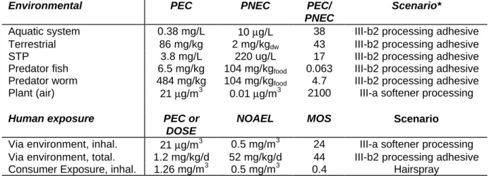
(14) page 14 of 60. RIVM report 679102 049. 5.. Probabilistic assessment of DBP. 5.1. Introduction to DBP. DBP is a high-production volume chemical that is used mainly as plasticiser in resins and polymers such as polyvinyl chloride. Other usages include the use in printing inks, adhesives, sealants, nitrocellulose paints, film coatings and glass fibres. Furthermore, DBP is ubiquitous in cosmetic consumer products. This chemical was selected as it is currently discussed in the existing chemicals framework and because it does not pose too many problems for EUSES (it is a neutral organic chemical). The analysis presented in Section 5.2 to 5.4 is based on the draft risk assessment report (RAR) of November 1998. In this draft, the emission data for 1997 were used. Our calculations, however, were made with the production and use figures from 1994 (as these were more complete at the time). To allow for a comparison between probabilistic and deterministic risk assessments, we recalculated the deterministic data with EUSES. The values in Table 1 therefore differ from the values given in the draft RAR. In Sections 5.5-5.6, a new risk assessment is made using the latest available data (RAR of 3 May 1999) was used with the emission data for 1998. More information on the probability distributions that were used can be found in Appendix 2.. 5.2. Conclusions of the dossier and EUSES. In Table 1 the highest risk ratios and lowest MOS values for DBP are shown as calculated with 1994 production data. Clearly, on the basis of this data set, there is reason for concern for all endpoints except fish-eating predators. Especially effects on plants through the atmosphere is a crucial endpoint. Table 1 Deterministic risk characterisation ratios (RCR) from EUSES for DBP calculated with 1994 data from RAR 17 November 1998. Environmental. PEC. PNEC. Aquatic system Terrestrial STP Predator fish Predator worm Plant (air). 0.38 mg/L 86 mg/kg 3.8 mg/L 6.5 mg/kg 484 mg/kg 3 21 µg/m. Human exposure. PEC or DOSE 21 µg/m3 1.2 mg/kg/d 1.26 mg/m3. Via environment, inhal. Via environment, total. Consumer Exposure, inhal.. 10 µg/L 2 mg/kgdw 220 ug/L 104 mg/kgfood 104 mg/kgfood 3 0.01 µg/m. PEC/ PNEC 38 43 17 0.063 4.7 2100. III-b2 processing adhesive III-b2 processing adhesive III-b2 processing adhesive III-b2 processing adhesive III-b2 processing adhesive III-a softener processing. NOAEL. MOS. Scenario. 24 44 0.4. III-a softener processing III-b2 processing adhesive Hairspray. 3. 0.5 mg/m 52 mg/kg/d 0.5 mg/m3. * The scenario code is the one that is used in the RAR.. Scenario*.

(15) RIVM report 679102 049. 5.3. page 15 of 60. Probabilistic risk assessment. Separate probability distributions are made for the local risk assessments (for each step of the life-cycle) and the regional assessment. Furthermore, where appropriate, the RCR on the basis of the available measured data is also shown in the same figure. The distribution of the measured values was taken as the best fitting log-normal distribution through all available data as given in the RAR. This distribution must be interpreted with care as the geographical relation between sources and sample sites was not clear. In the risk assessment report they were considered as “regional” concentrations. For each endpoint, a sensitivity analysis is given for the standard local scenario with the worst step of the life cycle (in this case processing). The sensitivities are presented as contribution of an input parameter’s uncertainty to the total uncertainty. Calculation is done by Crystal Ball by calculating the correlations between input sampling and the corresponding output. The parameters contributing at least 1% to the total variation of the RCR or PEC are shown. 5.3.1. Aquatic ecosystem. 100%. 100%. 90%. 90% 80%. prod.. 70%. form.. 60%. proc. regional. 50%. measured. 40%. RCR=1. 30%. 90 perc. max RCR. 20% 10%. cumulative probability. cumulative probability. 80%. prod.. 70%. form.. 60%. proc. regional. 50%. measured. 40%. PNEC. 30%. 90 perc. max PEC. 20% 10%. 0%. 0% -6. -4. -2. 0. 2. 4. -10. log RCR aquatic. Sensitivities Assessment factor lab-eco Local emission to water Biodegradation in STP. -8. -6. -4. -2. log PEC water (kg/m3). 57.3% 35.2% 4.7%. Local emission to water Biodegradation in STP Koc. 86.8% 9.9% 1.0%. The probability distributions of the RCR are for the most part to the left of the vertical line RCR=1 (left figure). This means that it is unlikely (p < 5%) that the RCR will exceed unity1. Processing is the most critical life-cycle stage (this distribution is most to the right of the graph) and the regional model leads to the lowest RCRs. The main source of uncertainty in the RCR for the processing step is the assessment factor on the data used to extrapolate from the NOEC of the most sensitive species to an ecosystem in the field. Second important, and dominating uncertainty in the PEC, is the uncertainty in the emission to water. The PEC distribution seems to be a bit more critical (closer to the vertical PNEC line; right figure)) than the RCR distribution. This is a response to the fact that the deterministic PNEC is quite conservative (at the lower end of its assumed distribution). For the stage of processing, 1. One has to realise that this interpretation must be made given the realism of the scenario and given the appropriateness of the model assumptions. In case a processing facility is located on a river that runs dry each summer, the probability of RCR exceeding 1 is no longer negligible. These limitations must be kept in mind when interpreting these distributions..

(16) page 16 of 60. RIVM report 679102 049. the probability that PEC exceeds this PNEC is approximately 10%. The measured PEC is more or less comparable to the local assessments although the risk assessment report claims them to be not point-source related. This implies that the local scenarios are not extreme worst cases. In conclusion, there seems to be little reason for concern for the aquatic system considering that the applied scenario is a conservative one. For the standard exposure scenario, the processing step indicates borderline risk when the assessment is based on uncertainties in the PEC only. The RCR and the PEC calculated with EUSES (the short lines in the figures) are above the highest percentile of the distributions. This indicates that the degree of compounded conservatism in the EUSES estimate is high. 5.3.2. Terrestrial ecosystem. 100%. 100%. 90%. 90% 80% prod.. 70%. form. 60%. proc.. 50%. regional. 40%. RCR=1 90 perc.. 30%. max RCR. cumulative probability. cumulative probability. 80%. form. 60%. proc.. 50%. regional. 40%. PNEC 90 perc.. 30%. 20%. 20%. 10%. 10%. 0%. prod.. 70%. max PEC. 0% -6. -4. -2. 0. 2. 4. -12. log RCR terrestrial. Sensitivities Assessment factor inter-species Assessment factor lab-eco Koc Local emission to water Biodegradation in soil. -10. -8. -6. -4. log PEC soil (kg/kg). 35.9% 29.8% 15.1% 14.3% 2.0%. Local emission to water Koc Biodegradation in soil. 48.1% 44.8% 3.9%. The situation with regard to the terrestrial ecosystem is largely similar to the aquatic: little reason for concern although the processing step is borderline. The 90th percentile of the processing distribution is close to the risk limit in both graphs: the probability of RCR>1 (left figure) and PEC>PNEC (right figure) are both slightly less than 10%. The regional results are far below the critical levels. Uncertainties in the effects assessment dominate the total uncertainty. Of the uncertain parameters in the exposure assessment for processing, the local emission to water and Koc are most important. This implies that the uncertainty in the route via sludge is more important than via deposition from air. Again, EUSES estimates are conservative (close to, or exceeding the 100th percentile of the Monte Carlo samples generated by Crystal Ball)..

(17) RIVM report 679102 049. Micro organisms in the STP. 100%. 100%. 90%. 90%. 80%. 80%. 70%. prod.. 60%. form. proc.. 50%. RCR=1. 40%. 90 perc.. 30%. max RCR. cumulative probability. cumulative probability. 5.3.3. page 17 of 60. 70%. prod.. 60%. form. proc.. 50%. 90 perc.. 30%. max PEC. 20%. 20%. 10%. 10%. 0%. PNEC. 40%. 0% -6. -4. -2. 0. 2. 4. -7. log RCR micro-organisms. -6. -5. -4. -3. -2. log PEC effluent (kg/m3). Sensitivities Assessment factor acute-chronic Local emission to water Biodegradation in STP. 57.1% 35.6% 4.0%. Local emission to water Biodegradation in STP. 86.9% 9.9%. The estimated risk for micro-organisms is rather low. The probability that RCR>1 (left figure) or PEC>PNEC (right figure) is less than 5%. Nevertheless, the EUSES estimates indicate more reason for concern. Major uncertainties are in the effects assessment and the emission to water. 5.3.4. Atmospheric exposure of plants. 100%. 100%. 90%. 90%. form. 60%. proc. regional. 50%. measured. 40%. RCR=1. 30%. 90 perc. max RCR. 20% 10%. prod.. 80%. prod.. 70%. cumulative probability. cumulative probability. 80%. form.. 70%. proc. 60%. regional. 50%. measured. 40%. PNEC 90 perc.. 30%. max PEC. 20%. NEL (AF 1000). 10%. 0%. 0% -6. -4. -2. 0. 2. 4. -14. log RCR atmosphere. Sensitivities Assessment factor lab-eco Local emission to air. -12. -10. -8. -6. log PEC air (kg/m3). 61.7% 35.3%. Local emission to air. 97.6%. This endpoint is where the highest risks are, as indicated by EUSES (see Table 1). For the stage of processing, the probability that RCR>1 is more than 95% (left figure), the probability of PEC>PNEC is essentially 100% (right figure). Also the formulation stage is important: p(RCR>1)≈50%, and possibly the production stage: p(RCR>1)≈10%. These percentages are even higher when the exceedance of the deterministic PNEC are considered. This reason for concern is not an artefact of the exposure scenario: when the measured data are considered, the 90th percentile of the RCR is close to 1 and the probability that PEC>PNEC is 30%. The measured data are largely intermediate between the local and the.

(18) page 18 of 60. RIVM report 679102 049. regional estimates. Since the scenario for these measurements is not necessarily worst case, a 95th percentile may be more suitable than a 90th percentile1. The most important source of uncertainty lies with the assessment factor from laboratory data to the field situation. In the exposure assessment, the uncertainty in the local emissions to air dominates. Also shown in the right figure is a human NEL (the inhalatory NOAEL divided by 1000). Humans exposed via inhalation seems to be a less critical endpoint than toxic effects in plants. Nevertheless, the PEC distribution for processing exceeds this NEL for 95%. Even an assessment factor of 100 would lead to unacceptable RCRs. In conclusion, this endpoint can clearly be considered at risk and since the risk estimate is so high, refinement will be difficult. Most useful in refinement seems to be more detailed toxicity testing with plants to lower the uncertainty about the no-effect level. Second important, and dominating the exposure assessment is the emission to air. 5.3.5. Fish-eating predators. 100%. 100%. 90%. 90% 80% prod.. 70%. form. 60%. proc.. 50%. regional RCR=1. 40%. cumulative probability. cumulative probability. 80%. prod.. 70%. form.. 60%. proc. regional. 50%. PNEC (AF 10). 40%. 90 perc.. 30%. PNEC (CED5). 20%. 20%. max PEC. 10%. 10%. 90 perc. 30%. max RCR. 0%. 0% -6. -4. -2. 0. 2. 4. -12. log RCR fish-eaters (CED). Sensitivities fish-eater BCF fish Assessment factor inter-species Local emission to waste water Assessment factor lab-field. -10. -8. -6. -4. -2. log PEC fish (kg/kg). 80.6% 8.9% 5.2% 1.8%. BCF fish Local emission to waste water Biodegradation in STP. 90.5% 6.1% 1.0%. For the predating birds and mammals, the exposure scenario is such that half of the diet is sourced from the local environment and the other half from the region2. The distributions in the figures representing steps of the life cycle therefore include 50% from the region. An additional calculation shows the contribution from the region only. Although the distributions are very broad (owing mainly to a high uncertainty in the BCF) 1. The interpretation of the percentiles hinges on the underlying uncertainties and scenarios. The local estimates represent a hypothetical worst case situation (100 m from the main point source). Measured data represent a more realistic scenario and one may want to have more certainty that this does not lead to exceedance of the PNEC. For the rather optimistic, highly averaged, scenario of the regional model a much higher percentile (e.g. 95 or 99%) should be considered. Please note that the distribution of the measured PEC represents mostly spatial and temporal variability whereas the uncertainty in the estimates represents operational uncertainty from the input parameters. 2 This was done to accommodate the fact that the feeding range of many species will exceed the boundaries of the local scale. The 50-50 division is quite arbitrary..

(19) RIVM report 679102 049. page 19 of 60. the probability of RCR>1 (left figure) or PEC>PNEC (right figure) is 5% or less1. This means that there is little reason for concern for these endpoints. Interestingly, the EUSES estimate for fish-eating predators is not very conservative. This is mainly due to the fact that we took all the available BCFs in a distribution whereas the dossier selects a very low one as most appropriate (see Appendix 2.2). The BCF distribution is the main source of uncertainty. This is not surprising as reported BCFs range from 10 to 7000 L/kg. 5.3.6. Worm-eating predators. 100%. 100%. 90%. 90% 80% prod.. 70%. form. 60%. proc.. 50%. regional RCR=1. 40%. cumulative probability. cumulative probability. 80%. prod.. 70%. form.. 60%. proc. regional. 50%. PNEC (AF 10). 40%. 90 perc.. 30%. PNEC (CED5). 20%. 20%. max PEC. 10%. 10%. 90 perc. 30%. max RCR. 0%. 0% -6. -4. -2. 0. 2. 4. -10. log RCR worm-eater (CED). Sensitivities worm-eater BCF worm Assessment factor inter-species Local emission to water Biodegradation in soil Koc Assessment factor lab-field. -8. -6. -4. -2. log PEC worm (kg/kg). 44.5% 27.1% 10.1% 5.6% 4.4% 3.2%. BCF worm Local emission to water Biodegradation in soil Koc. 66.1% 15.0% 8.2% 6.6%. For this endpoint, the local scenarios include 50% of the diet sourced from the region. The contribution of the region is also shown as a separate distribution. The probabilities for RCR>1, PEC>PNEC are 5% or less, indicating little reason for concern. The EUSES estimate is quite conservative and is located between the 95th and 100th percentile. The same PNECs are used as for the fish eating predators. These distributions are narrower than those for the fish-eating predators but are still quite broad (three orders of magnitude between 5th and 95th percentile). Main source of uncertainty is the BCF for earthworms which is derived from the QSAR training set.. 1. CED5 is the lower 5th percentile of the critical effects dose as estimated from the toxicological data. The PNEC (CED5) is based on this value with an assessment factor of 10. In this case, the difference between the PNEC and the CED5 is only a factor of four. The probabilistic RCR is based on the entire distribution of the CED and assessment factors for inter-species and lab-field differences. More information can be found in Appendix 2.3/2.4..

(20) page 20 of 60. 5.3.7. RIVM report 679102 049. Humans via the environment. 100%. 100%. 90%. 90% 80% prod.. 70%. form. 60%. proc.. 50%. regional. 40%. RCR=1 90 perc.. 30%. RCR (AF 1000). cumulative probability. cumulative probability. 80%. form.. 60%. proc. regional. 50%. NEL (AF 1000). 40%. NEL (CED5). 30%. 90 perc.. 20%. 20%. 10%. 10%. 0%. prod.. 70%. max DOSE. 0% -6. -4. -2. 0. 2. 4. -12. log RCR human (CED). Sensitivities Assessment factor time-scale Assessment factor inter-species Local emission to air Assessment factor intra-species Leaf conductance. -10. -8. -6. -4. log DOSE total (kg/kg/d). 44.4% 25.8% 15.4% 6.5% 4.4%. Local emission to air Leaf conductance BCF fish BAF meat. 70.3% 22.0% 2.4% 1.0%. The distribution of the RCR reveals a borderline situation for the step of processing. The 90th percentile of the RCR is just below 1 (left figure), but the distribution has a long tail that extends all the way up to 26001. This means that there is a 10% probability that the (uncertain) critical effect dose (see Appendix 2.4) is exceeded in an adult person of 70 kg, consuming 1.2 kg of leaf crops per day, all derived from the soils at 100m from the processing facility (the main route of exposure is through leaf crops which in turn are mainly exposed through air). This is not a highly unlikely scenario when there are vegetable gardens in the neighbourhood. When there are no agricultural areas or gardens in the vicinity of this source, a 90% protection level can be considered acceptable. The deterministic MOS is in this case 44, indicating insufficient protection (see Table 1). Based on a fixed NEL (either using an AF of 1000 as used in the RAR or the lower 5% confidence level of the critical effects dose) the situation is worse, in particular for the stage of processing (right figure). The 5th percentile of the CED crosses the curve for processing at the 30th percentile. This means that there is a 70% probability that this level is exceeded in our hypothetical adult. If we adhere to the NOAEL and use an assessment factor of 1000, the probability of exceeding this NEL is more than 95%. The main sources of uncertainty are formed by the assessment factors to extrapolate from the experimental study to the human situation. In the exposure assessment, the main uncertainty is the local emission to air followed by the conductance of the leaf crops. In conclusion, whether there is a high risk depends on whether or not uncertainties in the effects assessment are accounted for as these dominate the total uncertainty. Nevertheless, because of the extreme right tail of the distribution, caution is required and more information seems desirable.. 1. This a-symmetric shape after log-transformation is probably related to the fact that human exposure via the environment sums the contributions from several food sources. Summing of (nearly) log-normal distributions could lead to such strangely skewed distributions..

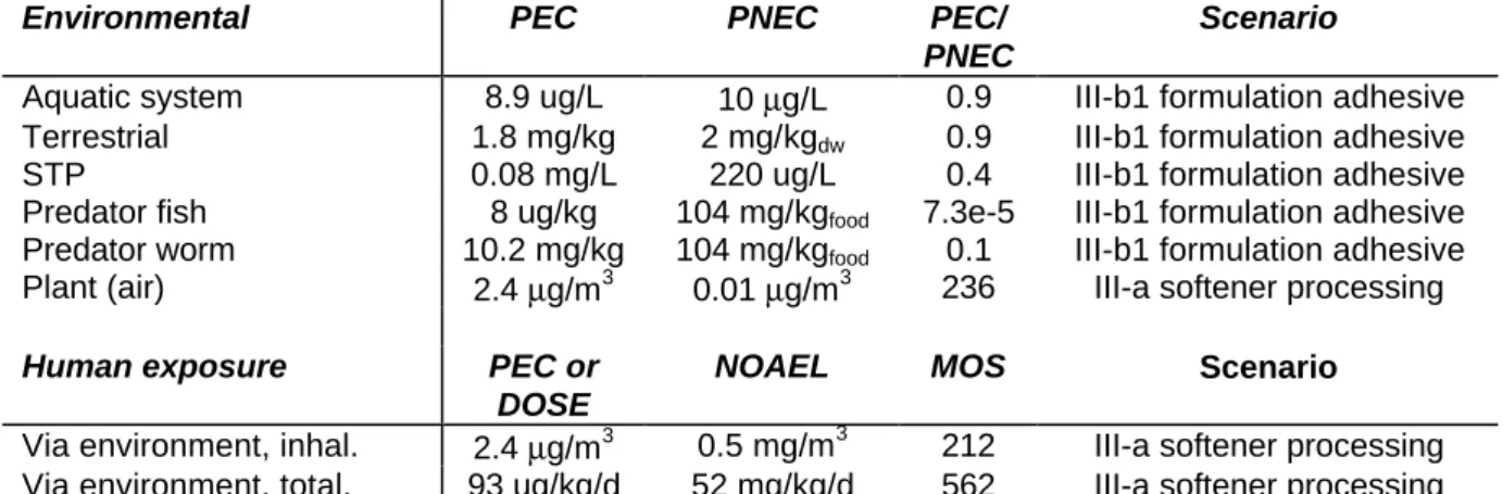
(21) RIVM report 679102 049. 5.4. page 21 of 60. Conclusions for DBP. Especially the risk assessment for the atmosphere (i.e. toxicity for plants via gas-phase exposure) and, to a lesser extent, exposure of humans via leaf crops are leading to serious concerns. Main possibilities for refinement can be found in the effects assessment for plants and humans and the local emissions to air at processing. Given the extent of risk observed for the atmospheric compartment, refinement must be quite extensive in order to achieve an acceptable risk. For the other endpoints, the probability that RCR exceeds 1 is less than 10%. In view of the conservatism of the exposure scenario, this seems acceptable. The EUSES estimates are quite worst case, (far) above the 95th percentile. This does not immediately imply that EUSES is too conservative. It depends on the uncertainties that we accounted for and the selected distributions. Nevertheless, the present results indicate that the TGD may be too protective, or at least, it must be considered that the results are certainly on the safe side.. 5.5. New data for DBP. The production and use of DBP has declined over the past years. In this section, the latest available data (RAR of 3 May 1999) was used and the emission data for 1998. Human effects data is currently being revised, therefore, no new data for this endpoint are used. For most of the endpoints, the RCRs could be pushed back below zero. Only the atmospheric exposure of plants remains a serious problem. Whereas in the previous Risk Assessment Report, processing was most important, now formulation has become the stage in the life cycle of highest concern. Only for plants, the processing step still dominates. In this section, the distributions will not be discussed in detail again as this was already done in the previous section. Here, the focus will be on the changes due to the newer data. Table 2 Deterministic risk characterisation ratios (RCR) from EUSES for DBP calculated with 1998 emission data (RAR version 3 May 1999). Environmental. PEC. PNEC. Aquatic system Terrestrial STP Predator fish Predator worm Plant (air). 8.9 ug/L 1.8 mg/kg 0.08 mg/L 8 ug/kg 10.2 mg/kg 2.4 µg/m3. Human exposure. PEC or DOSE 2.4 µg/m3 93 ug/kg/d. Via environment, inhal. Via environment, total.. 10 µg/L 2 mg/kgdw 220 ug/L 104 mg/kgfood 104 mg/kgfood 0.01 µg/m3. PEC/ PNEC 0.9 0.9 0.4 7.3e-5 0.1 236. Scenario III-b1 formulation adhesive III-b1 formulation adhesive III-b1 formulation adhesive III-b1 formulation adhesive III-b1 formulation adhesive III-a softener processing. NOAEL. MOS. Scenario. 0.5 mg/m3 52 mg/kg/d. 212 562. III-a softener processing III-a softener processing.

(22) page 22 of 60. 5.5.1. RIVM report 679102 049. Aquatic ecosystem. 100%. 100%. 90%. 90% prod.. 70%. form.. 60%. proc. regional. 50%. measured. 40%. RCR=1. 30%. 90 perc.. cumulative probability. cumulative probability. 80%. max RCR. 20%. prod.. 80%. form.. 70%. proc. regional. 60%. measured. 50%. PNEC. 40%. 90 perc.. 30%. max PEC. 20% 10%. 10%. 0%. 0% -6. -4. -2. 0. 2. -10. 4. -8. -6. -4. -2. log PEC water (kg/m3). log RCR aquatic. Sensitivities Assessment factor lab-eco Local emission to water Biodegradation in STP Koc. 62.6% 28.7% 4.6% 1.5%. Local emission to water Biodegradation in STP Koc. 84.3% 11.7% 1.4%. Risk is limited as the probability of RCR>1 and the probability that PEC>PNEC are less than 5%. The distributions have only been very slightly shifted to the left. 5.5.2. Terrestrial ecosystem. 100%. 100%. 90%. 90% prod.. 80% prod.. 70%. proc. 60%. form.. 50%. regional. 40%. RCR=1 90 perc.. 30%. max RCR 20%. cumulative probability. cumulative probability. 80%. form.. 70%. proc. 60%. regional. 50%. PNEC. 40%. 90 perc. max PEC. 30% 20% 10%. 10%. 0%. 0% -6. -4. -2. 0. 2. -12. 4. -8. -6. -4. log PEC soil (kg/kg). log RCR terrestrial. Sensitivities Assessment factor inter-species Assessment factor lab-eco Koc Local emission to water Biodegradation in soil. -10. 35.9% 32.4% 13.7% 12.2% 2.4%. Koc Local emission to water Biodegradation in soil. 49.0% 41.8% 6.1%. These distributions have also moved slightly to the left. The maximum exceedance of RCR=1 or the PNEC is less than 5%, which can be interpreted as “no reason for concern”..

(23) RIVM report 679102 049. Micro-organisms in STP. 100%. 100%. 90%. 90%. 80%. 80%. 70%. prod.. 60%. form. proc.. 50%. RCR=1. 40%. 90 perc.. 30%. max RCR. cumulative probability. cumulative probability. 5.5.3. page 23 of 60. 70%. prod.. 60%. form. proc.. 50%. 90 perc.. 30%. max PEC. 20%. 20%. 10%. 10%. 0%. PNEC. 40%. 0% -6. -4. -2. 0. 2. 4. -7. log RCR micro-organisms. -6. -5. -4. -3. -2. log PEC effluent (kg/m3). Sensitivities Assessment factor acute-chronic Local emission to water Biodegradation in STP. 62.7% 30.0% 4.3%. Local emission to water Biodegradation in STP Koc. 84.5% 11.7% 1.2%. Again, slightly shifted distributions which sets the maximum risk levels at less than 5%. 5.5.4. Atmospheric exposure of plants. 100%. 100%. 90%. 90%. form. 60%. proc. regional. 50%. measured. 40%. RCR=1. 30%. 90 perc. max RCR. 20% 10%. prod.. 80%. prod.. 70%. cumulative probability. cumulative probability. 80%. form.. 70%. proc. 60%. regional. 50%. measured. 40%. PNEC 90 perc.. 30%. max PEC. 20%. NEL (AF 1000). 10%. 0%. 0% -6. -4. -2. 0. 2. 4. -14. log RCR atmosphere. Sensitivities Assessment factor lab-eco Local emission to air. -12. -10. -8. -6. log PEC air (kg/m3). 67.4% 29.7%. Local emission to air. 97.6%. Analysis of the new data improves the situation only marginally. This endpoint is still of highest concern, especially for the stage of processing (although the other stages, as well as the measured data, do not provide an entirely safe situation). For processing, the probability of RCR>1 is approximately 95%, the probability that PEC>PNEC is effectively 100%. Clearly, there is a need for further study on this endpoint. The main uncertainty is in the lab-eco assessment factor and the emission to air but it should be noted that the total uncertainty is not very large. In fact, an acceptable risk can only be achieved when further studies yield parameter values beyond the range of the probability distributions currently applied. One should note that the PEC for this endpoint is not very conservative (at the 75th percentile). Also shown is a human NEL (the inhalatory NOAEL divided by 1000), which is less stringent than the plant PNEC, but is also exceeded at the stage of processing..

(24) page 24 of 60. 5.5.5. RIVM report 679102 049. Fish-eating predators. 100%. 100%. 90%. 90% 80% prod.. 70%. form. 60%. proc.. 50%. regional RCR=1. 40%. 90 perc. 30%. max RCR. cumulative probability. cumulative probability. 80%. form.. 60%. proc. regional. 50%. PNEC (AF 10). 40%. 90 perc.. 30%. PNEC (CED5). 20%. 20%. 10%. 10%. 0%. prod.. 70%. max PEC. 0% -6. -4. -2. 0. 2. 4. -12. log RCR fish-eaters (CED). -10. -8. -6. -4. -2. 0. log PEC fish (kg/kg). Sensitivities BCF fish Assessment factor inter-species Local emission to water Assessment factor lab-field. 82.4% 9.3% 4.4% 1.3%. BCF fish Local emission to water Biodegradation in STP. 92.2% 4.9% 1.0%. Again, we see the distributions shifted slightly to the left. The distributions are very broad but the probability of RCR>1 and PEC>PNEC are <5%. In this assessment, EUSES is definitely not conservative, as the deterministic quotient lies at the 25th percentile. This is caused by the fact that a very low BCF was selected in the update of the dossier (1.8 instead of 41.8 L/kg). The reasons for this choice are not entirely clear from the RAR. 5.5.6. Worm-eating predators. 100%. 100%. 90%. 90% 80% prod.. 70%. form. 60%. proc.. 50%. regional RCR=1. 40%. 90 perc. 30%. max RCR. cumulative probability. cumulative probability. 80%. form.. 60%. proc. regional. 50%. PNEC (AF 10). 40%. 90 perc.. 30%. PNEC (CED5). 20%. 20%. 10%. 10%. 0%. prod.. 70%. max PEC. 0% -6. -4. -2. 0. 2. 4. -10. log RCR worm-eater (CED). Sensitivities BCF worm Assessment factor inter-species Local emission to water Biodegradation in soil Koc Assessment factor lab-field Deposition rate gas phase. -8. -6. -4. -2. log PEC worm (kg/kg). 44.5% 27.7% 9.9% 5.1% 4.7% 2.9% 1.0%. BCF worm Local emission to water Koc Biodegradation in soil Deposition rate gas phase. The distributions are very broad but the probability of RCR>1 and PEC>PNEC are <5%.. 65.3% 13.2% 8.4% 6.7% 1.9%.

(25) RIVM report 679102 049. 5.5.7. page 25 of 60. Humans. 100%. 100%. 90%. 90% 80% prod.. 70%. form. 60%. proc.. 50%. regional. 40%. RCR=1 90 perc.. 30%. RCR (AF 1000). cumulative probability. cumulative probability. 80%. form.. 60%. proc. regional. 50%. NEL (AF 1000). 40%. NEL (CED 5%). 30%. 90 perc.. 20%. 20%. 10%. 10%. 0%. prod.. 70%. max DOSE. 0% -6. -4. -2. 0. 2. 4. -12. log RCR human (CED). Sensitivities Assessment factor time scale Assessment factor inter-species Local emission to air Assessment factor intra-species Leaf conductance. -10. -8. -6. -4. log DOSE total (kg/kg/d). 47.2% 26.8% 11.1% 6.0% 5.1%. Local emission to air Leaf conductance BCF fish BAF meat. 61.9% 29.8% 2.1% 1.5%. The situation for humans has improved slightly. For the processing stage, the probability of RCR>1 has gone below 5% although the tail extends up to an RCR of 130. When adhering to the fixed NELs, there is still an obvious risk situation for this chemical for processing (the probability that the CED5 is exceeded is approximately 40%). The reason for this diverging conclusions is the large uncertainty in the effects assessment. The other stages give little reason for concern. The deterministic PEC is very optimistic at 25th percentile of the distribution. Air is the main exposure of plant, which is the main source for human exposure, but the PEC for air was at the 75th percentile. The reason for this discrepancy is that we selected distributions for water solubility and vapour pressure. The medians of these parameters differ from those in the dossier in such a way that we got a much lower air-water partition coefficient (more than a factor of 10 with the median parameters values). This is a very important parameter for the airplant partitioning, leading to higher values in plants than the value in the dossier. It should be noted that the median value of our plant-water partition coefficient is very high (at the top of the experimental range reported in a validation study (Polder et al., 1997) and may be unrealistic as it is extremely dependent on small changes in physico-chemical properties. Nevertheless, this stresses the importance of uncertainty analysis since the choice of vapour pressure and water solubility is so important!.

(26) page 26 of 60. 5.6. RIVM report 679102 049. Alternative scenarios for DBP (new data). 5.6.1. Aquatic ecosystem. 100%. 100% 90%. proc.. 80%. regional. 70%. Dil=2. 60%. no STP/Dil=2 Dil=1e4. 50%. RCR=1 40%. 90 perc.. 30%. max RCR. cumulative probability. cumulative probability. 90%. regional. 70%. Dil=2 no STP/Dil=2. 60%. Dil=1E4 50%. PNEC. 40%. 90 perc.. 30%. max PEC. 20%. 20%. 10%. 10%. 0%. proc.. 80%. 0% -6. -4. -2. 0. log RCR aquatic. 2. 4. -10. -8. -6. -4. -2. log PEC water (kg/m3). Alternative scenarios are: Dil=2 dilution factor set to 2; indicating a very small stream no STP/Dil=2 dilution factor set to 2 and no sewage treatment; absolute worst case Dil=1e4 dilution factor set to 10000; indicating a large river Only the stage of processing is used for the alternative scenarios; the regional values are shown as reference. The choice of a dilution factor is quite important. The absolute worst-case scenario without STP is a definite risk situation. This means that we may have a problem when a processing site (or probably the also a formulation or production site) would discharge his effluent directly on such a small stream. With an STP, however, the RCR will stay below one but there is still a 30% probability that PEC exceeds the fixed PNEC. Interestingly, the width of the probability distributions is approximately two orders of magnitude (5-95%) but the difference between the best and worst-case scenarios is four orders of magnitude. This implies that the choice for an exposure scenario is potentially more important than the operational uncertainty in the input parameters..

(27) RIVM report 679102 049. 5.6.2. page 27 of 60. Terrestrial ecosystem. 100%. 100% 90%. proc.. 80%. regional. 70%. foc h/rain h foc l/rain l. 60%. no sludge 50%. RCR=1. 40%. 90 perc.. 30%. max RCR. cumulative probability. cumulative probability. 90%. regional. 70%. foc h/rain h foc l/rain l. 60%. no sludge 50%. PNEC. 40%. 90 perc.. 30%. max PEC. 20%. 20%. 10%. 10%. 0%. proc.. 80%. 0% -6. -4. -2. 0. log RCR terrestrial. 2. 4. -12. -10. -8. -6. -4. log PEC soil (kg/kg). Alternative scenarios are: foc h/rain h high fraction organic carbon in soil (30%), high rain rate (4 times normal) foc l/rain l low fraction organic carbon in soil (0.1%), low rain rate (1/4 times normal) no sludge normal Foc content but no sludge applied as fertiliser Changing the rain rate had no influence on the model results whatsoever as degradation was the primary removal process in soil. The scenario with high rain rate is combined with high organic carbon content (Foc) as these both tended to work to decrease the RCR. Changing Foc changes the soil sorption and hence the bioavailability of the compound. In the assessment, we assumed that Foc effects biodegradation and the PNEC linearly. A high Foc therefore leads to higher PECs (lower degradation) but high Foc leads to lower RCRs as the PNEC is lowered. In this way, the effects nearly cancel each other out in the RCR, but not in the PEC (in this graph, the vertical line representing the PNEC should shift with Foc which is not shown). The different scenarios affect the distributions less than for the aquatic environment..

(28) page 28 of 60. 5.6.3. RIVM report 679102 049. Regional systems. Alternative scenarios are (see Appendix 2.5): regional 2 same as regional but with temperature correction Spain Spanish country definition Finland Finnish country definition Aquatic ecosystem 100%. 100% 90%. proc.. 80%. regional. 70%. regional 2 Spain. 60%. Finland 50%. RCR=1. 40%. 90 perc.. 30%. max RCR. 80% cumulative probability. cumulative probability. 90%. regional 2. 60%. Spain. 50%. Finland. 40%. 90 perc.. 30%. 20%. 20%. 10%. 10%. 0%. regional. 70%. 0% -7. -6. -5. -4. -3. -2. -10. log RCR aquatic. -9. -8. -7. log PEC water (kg/m3). The result of the regional 2 scenario are virtually the same as the standard regional scenario. This implies that the temperature correction for vapour pressure and water solubility do not affect the fate of this chemical significantly. The difference between the countries is not very large. Finland is the most optimistic, a factor of 10 less than the standard regional system. Spain is somewhat worse than Finland which can be caused by the lower connection percentage to STPs, but still better than the standard region. Playing with the system settings revealed that the standard regional scenario is a kind of worst case because the emission is relocated to such a small area. This implies that size of the system needs to be carefully considered. Country borders may not be the most ideal choice, as national borders do not hamper the distribution of the chemical. To allow for a better comparison, another assessment was made with these extreme countries but with the same size as the standard region (Spain 2 and Finland 2 in the figures below). 100%. 100%. 90%. 90% proc. regional. 70%. Spain 2. 60%. Finland 2. 50%. RCR=1. 40%. 90 perc. max RCR. 30%. 80% cumulative probability. cumulative probability. 80%. 70%. regional. 60%. Spain 2. 90 perc. 40% 30%. 20%. 20%. 10%. 10%. 0%. Finland 2. 50%. 0% -7. -6. -5. -4. log RCR aquatic. -3. -2. -10. -9. -8. log PEC water (kg/m3). -7.

(29) RIVM report 679102 049. page 29 of 60. From these figures it is clear that the Spanish system is more at risk because of the low connection percentage to STPs. The Finnish system has lower concentrations because of the slightly higher connection percentage and probably because the water is much deeper. Still, the difference between the average concentrations in these systems is only a factor of 5.5. Terrestrial ecosystem 100%. 90%. proc.. 90%. 80%. regional. 80%. 70%. regional 2 Spain. 60%. Finland 50%. RCR=1. 40%. 90 perc.. 30%. max RCR. cumulative probability. cumulative probability. 100%. regional 2 60%. Spain. 50%. Finland. 40%. 90 perc.. 30%. 20%. 20%. 10%. 10%. 0%. regional. 70%. 0% -8. -7. -6. -5. -4. -3. -2. -13. log RCR terrestrial. -12. -11. -10. -9. log PEC soil (kg/kg). Again, the differences are not very large. The standard regional system is similar to Finland with respect to the distributions, Spain is a factor of 10 lower. This is probably caused by fact that degradation is more rapid and because there are less STPs and thus less sludge can be applied to soil as fertiliser. Again, these results are confounded with the different size of the system. When the standard regional size is used for the two countries (see Figure below), Spain has only slightly lower concentrations, but Finland is somewhat higher (due to the slower degradation rates). The difference in average PEC between the countries is a factor of 8.8. 100%. 100%. 90%. 90% proc. regional. 70%. Spain 2. 60%. Finland 2. 50%. RCR=1 90 perc.. 40%. max RCR 30%. 80% cumulative probability. cumulative probability. 80%. 70%. regional. 60%. Spain 2. 90 perc. 40% 30%. 20%. 20%. 10%. 10%. 0%. Finland 2. 50%. 0% -8. -7. -6. -5. -4. log RCR terrestrial. -3. -2. -13. -12. -11. -10. log PEC soil (kg/kg). -9.

(30) page 30 of 60. RIVM report 679102 049. Atmosphere 100%. 100%. 90%. 90% 80%. proc.. 70%. regional. 60%. regional 2 Spain. 50%. Finland. 40%. RCR=1. 30%. 90 perc.. cumulative probability. cumulative probability. 80%. max RCR. 20%. 70% regional 60%. regional 2. 50%. Spain. 40%. Finland 90 perc.. 30% 20%. 10%. 10%. 0%. 0% -6. -5. -4. -3. -2. -1. 0. 1. -14. log RCR atmosphere. -13. -12. -11. log PEC air (kg/m3). Here, Finland and Spain give similar results but the standard region is a factor of 5 worse. The main cause of this difference is probably that the regional system is smaller than the others. This is supported by the figures below where the all countries are the same size (figures below): since wind is the only removal mechanism and as the wind speeds are set equal in all countries, the concentrations in air are not affected. 100%. 100%. 90%. 90% 80% proc.. 70%. regional 60%. Spain 2. 50%. Finland 2. 40%. RCR=1 90 perc.. 30%. max RCR. 70% regional. 60%. Spain 2 50%. Finland 2. 40%. 90 perc.. 30%. 20%. 20%. 10%. 10%. 0%. 0% -6. -5. -4. -3. -2. -1. 0. 1. log RCR atmosphere. 5.7. cumulative probability. cumulative probability. 80%. -14. -13. -12. -11. log PEC air (kg/m3). Conclusions new data. With the new data, the situation for most endpoints has improved to an acceptable level of risk. However, for plants via the atmosphere, the situation still gives serious reason for concern. The probability of RCR>1 is very large (approximately 95%) which implies that serious study is required to see whether a reduction is possible by refining parameters. When the selected parameter distributions are a fair representation of the uncertainty, further studies will not get the RCR below one and emission reduction should be considered. However, when a more reliable study with plants can yield a toxicity value that is less stringent than the lower bounds of the current distribution, refinement of the assessment is possible. For humans, there may also be a problem when looking at the fixed no-effect levels and refinement is desirable. Additional scenarios provide insight in the role of variability, which turned out to be especially relevant for the aquatic system. For the aquatic ecosystem, an unacceptable risk will occur when a processing facility is discharging its effluent directly on a small water body. It depends.

(31) RIVM report 679102 049. page 31 of 60. on the realism of this scenario whether this gives reason for concern. For this endpoint, the scenario choice is dominating the total uncertainty. For the terrestrial ecosystem, the RCR distribution is not influenced much by the different scenarios since PEC and PNEC are affected in different directions by a change in organic matter content. Non of the scenarios leads to an unacceptable risk in this preliminary assessment. The differences between the standard region and two extreme countries (Spain and Finland) remain within a factor of 10. The standard region is worse than the other countries due to its small size. When the sizes are set equal, the regional system is between the others. Spain is the worst case for water, Finland for soil, for the air compartment, the differences are negligible. It must, however, be noted that not all country-specific defaults were adjusted in this assessment (see Appendix 2.5)..

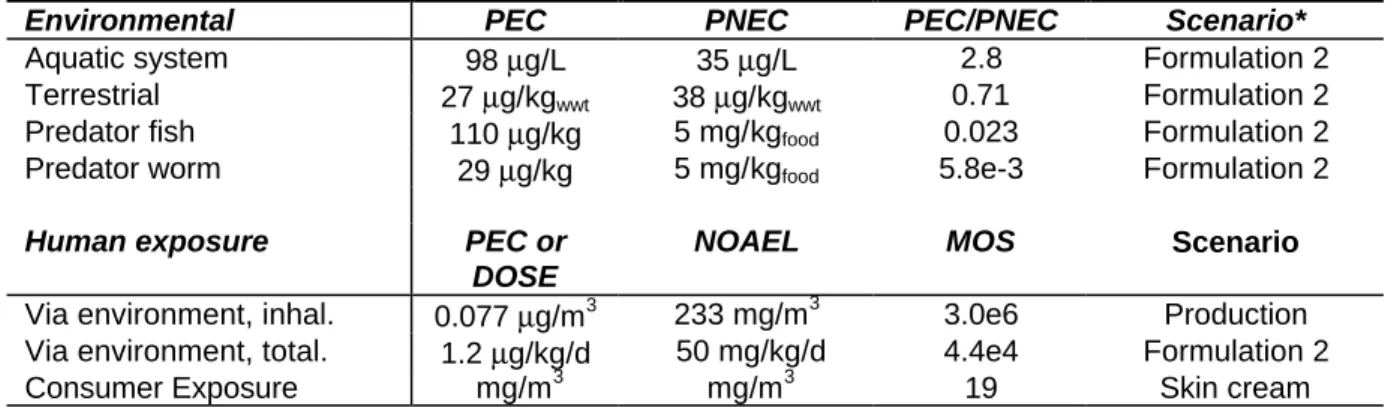
(32) page 32 of 60. RIVM report 679102 049. 6.. Probabilistic assessment of a new chemical. 6.1. Introduction to the new chemical. The selected chemical has recently been notified in the Netherlands. The chemical is used in the production of fragrances for soaps, cleaners and air fresheners. Apart from production and formulation, private use is a relevant life-cycle step. For production and formulation, 1 source is considered, for private use the 10% rule is applied (assuming 10% of the tonnage is used in the region and 90% in the continent).. 6.2. Conclusions of the dossier and EUSES. The exposure levels and the no-effect levels for this chemical are summarised in Table 3. For environment, conclusion ii was drawn (reason for concern, further information required at next tonnage threshold) because of the RCRs for the aquatic ecosystem and sediment 1 at production but especially at formulation. With regard to consumer exposure, immediate further information was required. Table 3 Deterministic risk characterisation ratios (RCR) from EUSES for the new chemical. Environmental Aquatic system Terrestrial Predator fish Predator worm. PEC 98 µg/L 27 µg/kgwwt 110 µg/kg 29 µg/kg. PNEC 35 µg/L 38 µg/kgwwt 5 mg/kgfood 5 mg/kgfood. PEC/PNEC 2.8 0.71 0.023 5.8e-3. Scenario* Formulation 2 Formulation 2 Formulation 2 Formulation 2. Human exposure. PEC or DOSE 0.077 µg/m3 1.2 µg/kg/d mg/m3. NOAEL. MOS. Scenario. 233 mg/m3 50 mg/kg/d mg/m3. 3.0e6 4.4e4 19. Production Formulation 2 Skin cream. Via environment, inhal. Via environment, total. Consumer Exposure. * For this chemical three formulation steps were identified. More information in Appendix 2.1.. Please note that the EUSES calculation is based on a production volume of 10 tons per year whereas the probabilistic assessment applies the current production volume.. 1. The sediment RCR is not shown in the table as it provides no extra information: both the concentration in sediment as well as the PNEC are derived by equilibrium partitioning from the water compartment. The reason that the RCRs for the aquatic and sediment are not entirely equal is that the PNEC is calculated with sediment properties whereas the PEC is calculated with the properties of suspended matter (i.e. freshly deposited matter)..

No results found