Fragmenting public transport timetables on the web in tiles for serverless route planning

(1)

in tiles for serverless route planning

Fragmenting public transport timetables on the web

Academic year 2019-2020

Master of Science in Computer Science Engineering

Master's dissertation submitted in order to obtain the academic degree of

Delva

Counsellors: Brecht Van de Vyvere, Julian Andres Rojas Melendez, Harm

Supervisors: Prof. dr. ir. Ruben Verborgh, Dr. Pieter Colpaert

Student number: 01401218

(2)

(3)

in tiles for serverless route planning

Fragmenting public transport timetables on the web

Academic year 2019-2020

Master of Science in Computer Science Engineering

Master's dissertation submitted in order to obtain the academic degree of

Delva

Counsellors: Brecht Van de Vyvere, Julian Andres Rojas Melendez, Harm

Supervisors: Prof. dr. ir. Ruben Verborgh, Dr. Pieter Colpaert

Student number: 01401218

(4)

Acknowledgements

First and foremost I would like to thank Dr. Pieter Colpaert for the inspiration his research gave me, his enthusiastic and passionate speeches and his continued motivational support. Next, also a thank you to Julian Rojas Melendez for his work on the Linked Connections Server and his patience when I got stuck. Thank you Harm Delva for always being available to answer my questions. Thank you Dylan Van Assche for providing me with your query set in an easy to use format. Thank you Pieter-Jan Vandeberghe for sharing his ideas on his thesis and letting me use his work as inspiration. Thank you to the research group for providing a space where I could work on my thesis and an endless supply of coffee. Thank you to Ghent University for granting me this opportunity. Thank you to everybody in my environment for supporting me throughout the past year.

Jeroen Flipts

(5)

Permission

The author gives permission to make this master dissertation available for consultation and to copy parts of this master dissertation for personal use. In all cases of other use, the copyright terms have to be respected, in particular with regard to the obligation to state explicitly the source when quoting results from this master dissertation.

(6)

Abstract

The ideal public transport route planners combine data from multiple sources, like train and bus schedules. As different groups of users have different requirements – such as accessibility or particular modes of transport – they need to be highly customizable. In recent years, services have arisen that integrate various sources and are able to provide fast response times, but are lacking in features and personalization. As more datasets are added and queries are increasingly more complex, it becomes inefficient for a server-side route planner to handle each individual request. With datasets being published as Linked Data Fragments, client route planners could solve these problems, but they introduce new complications like bandwidth and performance constraints. Improvements to this setup are twofold: (1) data should be published efficiently, but granular (2) so that clients have fine grained control over the data that needs to be fetched and processed. This thesis introduces two techniques for spatiotemporal fragmentation of Linked Open Data in the Linked Connections format and evaluates fragment selection techniques on accuracy, data usage and query time. Analysis of the results shows that for the used client-server combination up to 67% reduction in mean public transport data usage can be achieved, while maintaining adequate accuracy. However, only minimal improvements in query time have been measured. Based on these results, it can be concluded that spatiotemporal fragmentation of public transport data can improve bandwidth requirements of client side route planners. Additional research into more complex fragment selection techniques is required to further improve accuracy.

(7)

Fragmenting public transport timetables on the web in tiles for

serverless route planning

Jeroen Flipts

Supervisor(s): Prof. dr. ir. Ruben Verborgh, Dr. Pieter Colpaert, Julian Andres Rojas Melendez, Harm Delva, Brecht Van de Vyvere

Abstract— The ideal public transport route planners combine data from multiple sources, like train and bus schedules. As different groups of users have different re-quirements – such as accessibility or particular modes of transport – they need to be highly customizable. In recent years, services have arisen that integrate various sources and are able to provide fast response times, but are lacking in features and personalization. As more datasets are added and queries are increasingly more com-plex, it becomes inefficient for a server-side route planner to handle each individual request. With datasets being published as Linked Data Fragments, client route plan-ners could solve these problems, but they introduce new complications like bandwidth and performance constraints. Improvements to this setup are twofold: (1) data should be published efficiently, but granular (2) so that clients have fine grained control over the data that needs to be fetched and processed. This thesis introduces two techniques for spatiotemporal fragmentation of Linked Open Data in the Linked Connections for-mat and evaluates fragment selection techniques on accuracy, data usage and query time. Analysis of the results shows that for the used client-server combination up to 67% reduction in mean public transport data usage can be achieved, while maintain-ing adequate accuracy. However, only minimal improvements in query time have been measured. Based on these results, it can be concluded that spatiotemporal fragmenta-tion of public transport data can improve bandwidth requirements of client side route planners. Additional research into more complex fragment selection techniques is re-quired to further improve accuracy.

Keywords—Fragmentation, Open Data, Linked Data, Linked Connections, Public Transport

I. INTRODUCTION

In today’s society, fast response times to seemingly trivial question like calculating the optimal public transport journey from A to B, are expected. In recent years tremendous leaps have been made that make it viable to calculate the answers to such queries in real-time. How-ever, current state of the art applications lack customizability and per-sonalization of public transport queries as different user groups have different expectations and requirements. Some might need to transfer in wheelchair accessible stations while others are only interested in the cheapest or fastest route. With more and more datasets being published as Linked Open Data, client side route planners could solve many of these problems, but they introduce new complications like bandwidth and performance constraints. This document aims to first analyse the shortcomings with the current client side route planners and then pro-pose a solution to some of these drawbacks.

First a brief summary of literature and important concepts is given. Many different ways exist to publish data on the web. However, few techniques allow the data to be discovered, understood and processed by machines without human interaction. The most prominent approach to do this is through the semantic web, which can be seen as an exten-sion of the world wide web. This is essentially an umbrella term for standards and data formats that make internet data machine readable. The main building block of the semantic web is the resource description framework (RDF), a way of modeling information on the web without needing to know the structure of the data. The core concept of RDF is the triple pattern, a relation between a subject, a predicate and an ob-ject. If common uniform resource identifiers (URI) are used to denote elements of triples, context can be embedded. Whereas RDF is used to relate subjects and objects, it does not specify how it should relate to ex-ternal data. Linked Data (LD) has been introduced to fill this gap and is more of a ruleset on how to use RDF rather than an exact specification. Over the years, many datatypes have received a LD equivalent. A data

specification developed for public transport data is Linked Connections (LC) [1]. In LC the elementary building block is a single connection that must at least have departure and destination stops and departure and destination times. If complete datasets are published as LC, then navigation for machines needs to be provided so that they can discover more if desired. This can be done with hypermedia controls such as specified by Hydra [2]. Yet, Hydra is limited as it offers no distinction between ordered and unordered collections, and there is no possibility for ordering along multiple axis. For this, the experimental Tree Ontol-ogy can be used [3], which can be seen as an index to a collection like an index to a database.

In order to support navigation of a collection, the collection should first be fragmented into multiple parts. As there are many different types of data, discussion on fragmentation strategies will be limited to geospatial data. This is data that can be mapped to a location, com-monly by specifying coordinates in a previously agreed upon coordi-nate system. A popular technique for fragmenting geospatial data is by tiling it on a grid based structure. Different approaches exist with Slippy tiles [4] being the most popular for road networks. The main ap-peal is that it can identify each tile by a simple human readable 3-tuple (zoom, x, y). Other tiling approaches are hierarchical binning [5] and hexagonal tiling [6], [7]. Finally, irregular shaped partitioning is also an option as shown by Bast e.a [8].

As fragmentation strategies are only as good as their fragment se-lection counterpart, these are equally important. However research on this topic is rather limited. Implicit fragment selection is employed by Strasser and Wagner [9] and in customizable road planning (CRP) [10], [11]. A different approach for fragment selection is used by the Valhalla route planner [12], but unfortunately no details are given.

As this document deals with public transport route planners, an overview of the state of the art is also given. Many different opti-mization criteria exist, but only a few are used regularly. Often these include some form of Pareto optimality [13] if used on multiple param-eters. Popular criteria are the earliest arrival problem [14], [15], [16], [17], multicriteria problem [17], earliest arrival profile problem [14] and Pareto profile problem [17],[14].

Bast [18] has presented several reasons why public transport rout-ing is much more difficult than road based routrout-ing. All state of the art public transport routing algorithms have to make compromises on ei-ther query speed, preprocessing time or optimality. Currently ei-there are three major alternatives, namely CSA [15], [14], [9], RAPTOR [17] and Transfer Patterns [19], [20], [8]

II. METHODS

The research performed has been split into two stages, in the first stage the shortcomings of a recent implementation of a route planning client - data server architecture are identified and in the second stage the implementations of both client and server are augmented to mitigate some of the problems identified.

The architecture under evaluation consists of the typescript Planner.js client [21] and the node.js Linked Connections Server [22], both of which are open source and freely available for adaption. The server converts datasets in the General Transit Feed Specification (GTFS) and

(8)

publishes them as Linked Data in the form of Linked Connections. These connections are sorted by departure time and paginated along the temporal axis for fast and granular axes. The planner then uses these connections as input for the route calculation algorithm. The algorithm used for the evaluation is the most basic version of CSA, which solves the earliest arrival problem. Core features of the Planner.js client are the support for multiple simultaneous data sources and the high cus-tomzability.

The shortcomings identified during this stage are:

• Large GTFS datasets are not converted to Linked Connections in a

time and space efficient way. Expensive server grade equipment is re-quired to convert country size bus networks such as that of De Lijn. The De Lijn GTFS dataset published on 3 December 2019 contains 36,191 stops, 1,410 routes and 315,591 trips over a period of 75 days, which results in millions of connections. As each Linked Connection in an uncompressed state has a size in the order of 1KB, this quickly adds up to dozens of GB during conversion. It is not hard to image even larger datasets for larger public transport providers.

• Some queries take a considerable amount of time to return a journey.

Users are not willing to wait for more than 30 seconds when server side journey calculation can be performed in less than a second. The problem becomes larger when bigger datasets are considered.

• Lastly, Colpaert e.a. (2017) [23] have shown that Linked

Connec-tions require 3 orders of magnitude higher bandwidth per connection compared to a traditional query server. Again this problem is exagger-ated when larger datasets are considered.

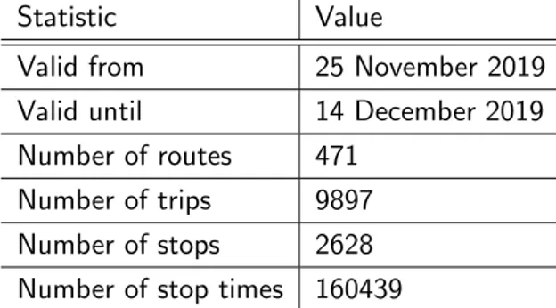
A common trend between the three stated problems is that perfor-mance is good for small datasets, but worsens when more data is avail-able. This is particularly troublesome as additional data does not nec-essarily impact optimal journeys. Even for country size train networks, like the NMBS, that are typically much smaller than bus networks, per-formance is not optimal. For example, the NMBS dataset of 1 De-cember has 2,628 stops, 471 routes and 9,897 trips, but queries can occasionally still take more than 30 seconds and consume several MB of data. As many users execute public transport queries on their mo-bile phone on momo-bile data, this is currently unacceptable as a proper alternative to server side route calculations.

Several reasons have been identified for the worsening performance depending on dataset size:

• Dataset conversion time and space complexity of the Linked

Con-nection Server is mostly a result of all the data being processed at once. First all Linked Connections are generated, then all of them are sorted and lastly they are paginated. However there is no need to process complete GTFS datasets at once as each page of connections is only dependent on a sliding window of sorted trips.

• Calculating journeys is inefficient in both time and space complexity

as CSA is designed to produce the optimal result. The larger the dataset, the more connections need to be scanned to produce the optimal jour-ney with the earliest arrival time. This requirement means that all con-nections between the departure and arrival time of the optimal journey are scanned, no matter where they are located in the network. Every scanned connection needs to be sent from server to client resulting in large data bandwidth usage. In efficient server side implementations of CSA, this is less noticeable through the use of Single Instruction Mul-tiple Data (SIMD) operations. However this is not possible on arbitrary client hardware.

• The specific Planner.js implementation can calculate routes between

arbitrary locations. If departure and arrival locations are not stops, but geographical coordinates, the planner has to calculate routes to the nearest stops. In case no stops are located nearby, this can take up a large portion of the final query time. Calculations of more than 20 sec-onds are no exception.

The problems are very diverse and can therefore not be solved with a single solution. Both the first and the third problem seem to be mostly implementational rather than technical. Therefore the choice has been

made to research solutions to the second problem which have been im-plemented during the build phase.

In order to mitigate the performance and data transfer bottlenecks in-troduced by scanning an excessive amount of connections, optimality has to be dropped. As connections are scanned that are not geograph-ically relevant to solve a public transport query, the proposition made in this document is to perform geospatial fragmentation. Doing this in combination with the already present temporal fragmentation gives route planning clients fine grained access to the data while the server can maintain high performance. This fine grained access in combina-tion with intelligent algorithms to decide on the required fragments, should make performance of clients less dependent on dataset size. In order to differentiate between spatial fragmentation and temporal frag-mentation, the latter will from now on be referred to as pagination.

The proposed solution thus consists of two separate parts:

• The Linked Connections need to be fragmented such that only a

small number of fragments are required to solve each query.

• A heuristic needs to be designed such that all required fragments are

selected.

The fragmentation strategy should be chosen in such a way to enable simple heuristics.

Road based planners are a source of inspiration for good fragmen-tation strategies. As they deal with vast quantities of data, they need to employ efficient fragmentation and use this to speed up route cal-culations. Typically, they fragment road networks into regular shaped hierarchical tiles of a grid. Larger tiles, close to the root, only contain abstractions of the road network, while lower level tiles contain more detail. While abstracting away Linked Connections is not straightfor-ward, they can still be fragmented into tiles. As tiling standard, Slippy tiles is chosen for its simplicity and widespread use in industry. Slippy tiles is a type of quadtree where each node in the tree can be identified by a 3-tuple (zoom, x, y). The zoom is equal to the depth of the node and starts at 0 for the tile covering the whole world. The x (y) value is the number of tiles to the left (above) the tile in question on that zoom level and are in the range 0 to 2zoom_{. Two different tiling strategies}

have been implemented. These are discussed in Section III-A.1. As clients could be dealing with datasets they are unfamiliar with, a technique is required to discover available tiles. Again two different approaches have been implemented which are discussed in Section III-A.2.

Lastly, several tile selection strategies have been realized which dif-fer depending on the used tile discovery strategy. On top of this, tile selection strategies that take a multistage approach have been consid-ered. Instead of one set of tiles, they produce multiple sets that result in consecutive executions of CSA. The different tile selection strategies are explained in Section III-B.

Finally the different allowed combinations need to be evaluated. The dataset chosen for evaluation is the previously mentioned NMBS dataset as it can be converted to Linked Connections in a timely man-ner while it exhibits the same performance problems, albeit to a smaller extent, as larger datasets. Each implemented combination of tiling tech-nique and tile selection strategy has been evaluated on accuracy, query time and query size. The impact on server side preprocessing is mea-sured as well. The results and discussion of these experiments can be found in Section IV.

III. IMPLEMENTATION

A. Tiled Linked Connections Server

Public transport service providers generally publish their time tables in the GTFS structure. As a GTFS data dump is not client friendly, the timetables should be converted to a data format more suitable for the web. Linked Connections is the format chosen for this and the Linked Connections Server is an experimental setup that can do both conversion from GTFS and then publish datasets. In order to create a

(9)

tiled version of this server, both the dataset converter stage and the web server need to be modified.

A.1 Tile Generation

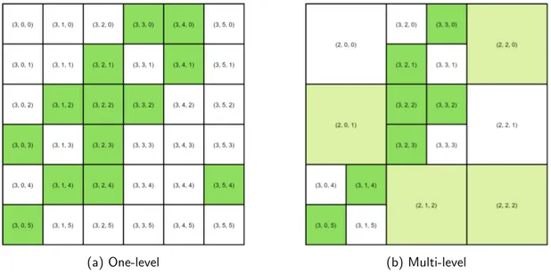
Two different tiling strategies have been implemented. As mentioned earlier, Slippy tiles is used as tiling grid and each tile can be identified by a 3-tuple (zoom, x, y). The first type of tiling fragments the data into tiles of equal geographical size and will be referred to as One-level Tiling as all 3-tuples have the same zoom level. Assuming the connec-tions are sorted by departure time, each connection is hashed to its tile id by using the departure stop as input to the hash function. During fragmentation, pagination is performed as well. In order to reduce the spread on the departure time of connections in a single page, a max-imum time window between the first and the last connection can be specified.

The second type fragments the data in tiles of multiple sizes with the aim to create tiles with similar density of connections. This strategy has been called Multi-level Tiling as different tiles can have different zoom levels. The larger tiles are created in a bottom up fashion starting from the one-level tiles. Four tiles with the same parent node in the Slippy tiles structure are iteratively combined if their combined size is below a threshold. This is repeated for each level until no more tiles can be combined, zoom level 0 is reached or a specified minimum zoom level is reached.

A.2 Tile Discovery

In addition to publishing tiled data, new techniques to discover the available tiles are required. Again, two different approaches have been implemented. The first is to provide an endpoint that publishes a cat-alog of all available tiles and is referred to as Static Discovery. The second takes a granular approach based on the experimental Tree On-tology and its GeospatiallyContainsRelation where all tiles can be dis-covered by following branches from a single root and will be referred to as Dynamic Discovery. Essentially, the tree can be seen as a multi-level index to all the tiles like an index in a database and is assembled from two types of nodes, namely internal nodes and leave nodes. The internal nodes are the indexes while the leave nodes are the tiles. Just like the tiles, internal nodes are identified by a Slippy tile 3-tuple. As a tile on one zoom level covers 4 tiles of the next zoom level, an internal node can contain up to 4 children. Children of internal nodes can either be internal nodes, leave nodes or a mixture of both.

Just like the implementation of the multi-level tiler, the tree is built bottom up from the deepest tiles. New internal nodes are introduced level by level making sure that all nodes of the next level are discover-able. This process is repeated until either level 0 is reached or all nodes can be reached from a single node. This last node becomes the root and acts as the entry point to the tree.

A.3 Web Server

In the web server, pages of connections can be fetched through the new

/ : agency/connections/ : zoom/ : x/ : y

endpoint. Navigation between the pages is done by following the Hy-dra hypermedia controls hyHy-dra:previous and hyHy-dra:next, and a specific page can be requested by providing a timestamp in the departureTime query parameter.

In case static discovery is used, the catalog is available through the / : agency/tiles

endpoint. If dynamic discovery is provided instead, the internal nodes are available through the same endpoint as the tiles as they have the same identifiers while the root of the tree is available on the

/ : agency/connections

endpoint as well. B. Planner.js Client

As the data published by the server is now spatially fragmented, the Planner.js client needs to be adapted to deal with this new type of source. Most importantly, it requires a strategy to select a set of tiles so that most queries can still be solved optimally without select-ing too much false positives. In order to properly measure the impact of the spatial fragmentation of the data, the decision has been made to keep the tile selection strategies as simple as possible. In total, three unique tile selection strategies have been implemented. Two of them select all tiles on a straight line between departure and destination stop where the difference is the used tile discovery technique. The strategy using static discovery has been named the Straight Line Tile Selection Strategy, whereas the strategy using dynamic discovery is referred to as the Tree Tile Selection Strategy. Lastly, the third strategy also uses static discovery and consists of multiple stages that produce expanding sets of tiles with the first stage being identical to the straight line tile selection strategy. Each of the next sets is made out of the previous set combined with all tiles that are adjacent to the previous set including tiles that do not exist. This last strategy is referred to as the Expanding Tile Selection Strategy.

IV. RESULTS ANDDISCUSSION

Results were obtained on a virtual machine running Ubuntu 18.04. The VM is assigned 4 logical processors of an i7-7700HQ, 8192 MB of DDR4 ram and 30 GB of storage on a 5400 rpm hard drive. All results are obtained on the NMBS GTFS dataset from 1 December 2019 with 100 queries randomly sampled from a set of real queries published by iRail. The dates and hours of the sample queries are modified so that they can be answered by the dataset.

By combining two tiling strategies with two discovery techniques and three tile selection strategies, 12 hypothetical setups are obtained. However, not all combinations can exist, like the tree tile selection strat-egy that requires dynamic discovery to access the tree. In total 5 com-binations of the Linked Connections Server and Planner.js instances are valid. These can be found in Table I.

TABLE I

THIS TABLE REPORTS VALID UNIQUE COMBINATIONS OF TILING TECHNIQUE,TILE DISCOVERY AND TILE SELECTION STRATEGY.

Tiling Technique Tile Discovery Tile Selection Strategy One-level Static Straight Line Tile Selection One-level Static Multistage Expanding Tile Selection One-level Dynamic Tree Tile Selection

Multi-level Static Straight Line Tile Selection Multi-level Dynamic Tree Tile Selection

A. Tiled Linked Connection Server

As could be deduced from Table I, at least 5 different Linked Con-nections datasets are required by all the different planners. One base-line dataset where no fragmentation is applied in addition to all possible combinations of one-level or multi-level fragmentation and static or dy-namic tile discovery. In total 6 tiled datasets have been generated with 3 sets of parameters. These can be found in Table II.

Some statistics on the generated tiled datasets can be found in Table III. For reference, the number of pages generated without tiling is 9202. When analysing these numbers, it is clear that the shorter maximum page length results in many more pages. However, the amount of tiles is much lower and therefore the internal structure of the tree is less complex.

During conversion of the datasets, the time taken up by each stage has been measured. These measurements are shown in Figure 1. As

(10)

TABLE II

SETS OF PARAMETERS USED DURING CONVERSION OF THE DATASET. Set Tiling Technique Max

Page Size Max Page Length Max Zoom Level Min Zoom Level Join Threshold 1 One-level Tiling 50 000 24h 12 2 Multi-level Tiling 50 000 24h 12 7 2 000 000 3 Multi-level Tiling 50 000 2h 12 7 8 000 000 TABLE III

NUMBER OF TILES AND INTERNAL NODES GENERATED AND SIZE OF RESPONSE OF THE AVAILABLE TILES ENDPOINT USED IN STATIC DISCOVERY. Set # Pages # Tiles # Internal Nodes /tiles Response Size [KB]

1 13098 322 281 63.3

2 12095 259 131 51.3

3 28083 135 57 27.5

each configuration has only been timed once, the measurements are not completely accurate. This can be seen in the initial stages that per-form identical computations for each configuration but have different timings. However, it is still clear that applying one-level fragmenta-tion has limited impact on the total conversion durafragmenta-tion and the impact of multi-level fragmentation largely depends on the parameters used. Lastly, building the tree for dynamic discovery has barely any notice-able impact at all.

Fig. 1. This stacked bar chart shows the dataset conversion times split into the different contributing parts. Each dataset has been generated once. An increase in conversion time can be noted for all tiling configurations over no tiling. The one-level tiling stage doubles compared to only performing pagination. The duration of the multi-level tiling stage largely depends on the specified parameters. Building the tree for dynamic dis-covery has no noticeable impact.

It is expected that most of the increase in duration can be attributed to an increased number of IO operations and overall decreased IO per-formance. Efficient implementations storing less intermediate results to the hard drive could further reduce the increase in dataset conversion time.

B. Planner.js Client

Before stating the results of the different planner configurations, it is important to mention that each query is ran independently. This means that the internal state of the planner is reset after each query and no fetched results can be shared between queries. If this would have been allowed, different results are expected, however less relevant as few clients will run 100 queries in quick succession.

B.1 Public Transport Query Duration

In Figure 2 the total duration for each query is reported. This is the duration measured from the instantiation of the Planner instance up to the closing of the asynchronous iterator of results. While the to-tal duration may give a good indication of the computational resources consumed, it is not necessarily in line with the user perceived perfor-mance. When analysing the results, each Planner server combination is marginally faster compared to the Planner without tiling except the Planner with the expanding tile selector. High durations are mostly at-tributed to processing of the routable tiles to find the nearest departure and arrival stops, while slowness of the expanding tile selector is due to inefficient implementation. In the implementation of the multistage tile selection strategy, no registry of fetched tiles is shared between the successive stages. This means that each stage needs to fetch the same pages as the previous stage already fetched. However, when this stage is evaluated on first and best result duration, similar durations as the others are achieved.

Fig. 2. This bar chart reports the mean, median and 5 and 95 percentiles durations for the total query durations for each combination of client and server. Only minimal reductions in total query times are measured compared to no tiling. The expanding query tile selection planner is slower, which can be attributed to its inefficient implementation.

B.2 Public Transport Query size

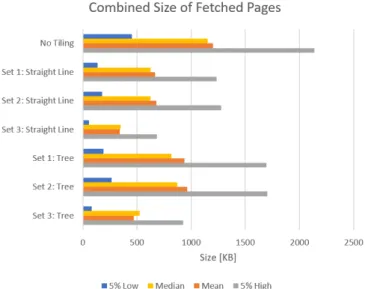
The second evaluation metric is the impact on total query size, which has been defined as the combined size of the fetched pages in addition to the size of the tile discovery overhead. The combined size of fetched pages can be found in Figure 3 and the size of the discovery overhead in Figure 4. The size of the expanding tile selection strategy applied on the dataset with parameter set 1 is not included as the results are unusable due to the inefficient implementation.

When analysing the total query size for the different planner config-urations, it is clear that much larger improvements have been achieved

(11)

Fig. 3. This bar chart reports the mean, median and 5 and 95 percentiles sizes for the combined size of all fetched pages. Both tile selection strategies have lower combined size of fetched pages than with tiling. This is the main contributing factor of the lower total query sizes.

Fig. 4. This bar chart reports the mean, median and 5 and 95 percentiles sizes for dynamic tile discovery and exact values for static tile discovery. Dynamic tile discovery has lower data overhead for most queries. Depending on the number of tiles, static tile discovery can perform better.

than with query duration. In some cases even the barrier of 50% total query size reduction is broken. Further reductions can be expected if the aggressive prefetching of the planner is toned down. The current sit-uation is that the next page will automatically be fetched if the current page is being read. The greatest improvements are seen for the planners using static tile discovery rather than those employing dynamic tile dis-covery. However, it should be noted that the dataset tiling configuration has a larger impact than the choice between these two for the used input dataset. Furthermore, the size of static tile discovery is linearly corre-lated with the number of tiles, while this is logarithmic for the dynamic tile discovery. As such, large datasets with lots of tiles will be more efficient with the dynamic variant.

B.3 Public Transport Query Accuracy

Finally, the last metric that the different planners have been evaluated on is query accuracy. As optimality of the CSA algorithm has been

dropped to perform the geospatial fragmentation, it is important that satisfactory journeys are still returned. For this, two types of accuracy have been calculated. First, there is the perfect accuracy that assumes a journey as accurate if it has the same arrival time as the optimal solution provided by the non tiled implementation of CSA. The second type of accuracy counts a result as accurate if the arrival time falls within a margin of error of the optimal result.

The results of the computed accuracies can be found in Figure 5. Even with the easiest tile selection strategy imaginable, all planners return in more than 80% of the cases the optimal journey. When com-paring the accuracies of the two tiling strategies, no noticeable differ-ences can be noticed when similar dataset parameters are used (set 1 and 2). However, choosing better parameters can slightly improve ac-curacy (set 3).

Fig. 5. This bar chart reports the computed accuracies of the different tile selecting strate-gies. The set of tiles selected by the tree tile selecting strategy is identical to the set of tiles selected by the straight line tile selecting strategy. Therefore the accuracy is not reported separately. All tile selection strategies achieve more than 80% accuracy. Most of the journeys found are either optimal or nearly optimal. Multistage expanding tile selection manages to find journeys the other tile selection strategies could not find.

From the accuracies two conclusions can be made.

• If a journey is found in the first stage, it is almost always a good one

and often a perfect one.

• If no journey is found, a second stage can be performed that uses a

much larger set of tiles and therefore has very high chances to find a result that is almost always optimal

V. CONCLUSION

The aim of this document is to assess if fragmenting a public trans-port timetable is viable for serverless route planning. First, weaknesses with the current Linked Data implementation of public transport query solvers have been identified. The stack under evaluation is the com-bination of the Linked Connections Server with the Planner.js client. The identified shortcomings are (1) the high time and space complexity of the dataset conversion, (2) slow query times, (3) relative high band-width usage. In a second stage, a technique for improving the third drawback has been proposed, of which several variants have been im-plemented. The compromise made to improve the bandwidth usage is that no proven accuracy can be achieved. Two fragmentation strategies have been designed: one-level and multi-level tiling. In order to dis-cover these newly created tiles, two tile disdis-covery approaches have been considered namely static and dynamic tile discovery. Finally, three sim-ple tile selection strategies have been imsim-plemented. Two straight line variants and one multistage technique.

In total five combinations of tiling, discovery and tile selection are valid. These have been tested on three metrics: query duration, query

(12)

size and accuracy. The results can be summarized as follows. Any gain in query duration is negligible as for each query most time is spent calculating the potential departure and arrival stops, which are not im-pacted by the proposed solutions. Up to 67% reduction in query band-width usage can be achieved, depending on the parameters used during tiling, while no clear advantage can be noted for either one-level or multi-level tiling. The choice for discovery strategy depends on the number of tiles and the complexity of the tiling structure with more tiles being in favor of dynamic discovery. Lastly, for over 80% of the queries, the first answered journey is optimal and almost all answered queries are optimal. If no journey is found during the first stage, later stages are likely to find a solution, which is nearly always optimal.

ACKNOWLEDGMENTS

This document has been written as part of a master’s theses. The author would like to thank his supervisors Prof. dr. ir Ruben Verborgh and Dr. Pieter Colpaert and counsellors Brecht Van de Vyvere, Julian Andres Rojas Melendez and Harm Delva for their guidance throughout this project and the received opportunity.

REFERENCES

[1] Pieter Colpaert, Alejandro Llaves, Ruben Verborgh, Oscar Corcho, Erik Mannens, and Rik Van de Walle, “Intermodal public transit routing using Linked Connections,” p. 5.

[2] “Hydra: Hypermedia-Driven Web APIs,” .

[3] Pieter Colpaert, “pietercolpaert/TreeOntology,” Nov. 2019, original-date: 2018-08-17T11:11:57Z. [4] “Slippy map tilenames - OpenStreetMap Wiki,” .

[5] rbrundritt, “Bing Maps Tile System - Bing Maps,” .

[6] Colin P. D. Birch, Sander P. Oom, and Jonathan A. Beecham, “Rectangular and hexagonal grids used for observation, experiment and simulation in ecology,” Ecological Modelling, vol. 206, no. 3, pp. 347–359, Aug. 2007.

[7] Isaac Brodsky, “H3: Uber’s Hexagonal Hierarchical Spatial Index,” June 2018.

[8] H. Bast, M. Hertel, and S. Storandt, “Scalable Transfer Patterns,” in 2016 Proceedings of the Eighteenth Workshop on Algorithm Engineering and Experiments (ALENEX), Proceedings, pp. 15– 29. Society for Industrial and Applied Mathematics, Dec. 2015.

[9] Ben Strasser and Dorothea Wagner, “Connection Scan Accelerated,” in 2014 Proceedings of the Sixteenth Workshop on Algorithm Engineering and Experiments (ALENEX), Catherine C. McGeoch and Ulrich Meyer, Eds., pp. 125–137. Society for Industrial and Applied Mathematics, Philadelphia, PA, May 2014.

[10] Daniel Delling, Andrew V. Goldberg, Thomas Pajor, and Renato F. Werneck, “Customizable Route Planning,” in Experimental Algorithms, Panos M. Pardalos and Steffen Rebennack, Eds., Berlin, Heidelberg, 2011, Lecture Notes in Computer Science, pp. 376–387, Springer.

[11] Daniel Delling and Renato F. Werneck, “Faster Customization of Road Networks,” in Experimental Algorithms, Vincenzo Bonifaci, Camil Demetrescu, and Alberto Marchetti-Spaccamela, Eds., Berlin, Heidelberg, 2013, Lecture Notes in Computer Science, pp. 30–42, Springer.

[12] “Why tiles? - Valhalla,” .

[13] A Charnes, W. W Cooper, B Golany, L Seiford, and J Stutz, “Foundations of data envelopment analysis for Pareto-Koopmans efficient empirical production functions,” Journal of Econometrics, vol. 30, no. 1, pp. 91–107, Oct. 1985.

[14] Julian Dibbelt, Thomas Pajor, Ben Strasser, and Dorothea Wagner, “Connection Scan Algorithm,” arXiv:1703.05997 [cs], Mar. 2017, arXiv: 1703.05997.

[15] Julian Dibbelt, Thomas Pajor, Ben Strasser, and Dorothea Wagner, “Intriguingly Simple and Fast Transit Routing,” in Experimental Algorithms, David Hutchison, Takeo Kanade, Josef Kittler, Jon M. Kleinberg, Friedemann Mattern, John C. Mitchell, Moni Naor, Oscar Nierstrasz, C. Pandu Ran-gan, Bernhard Steffen, Madhu Sudan, Demetri Terzopoulos, Doug Tygar, Moshe Y. Vardi, Ger-hard Weikum, Vincenzo Bonifaci, Camil Demetrescu, and Alberto Marchetti-Spaccamela, Eds., vol. 7933, pp. 43–54. Springer Berlin Heidelberg, Berlin, Heidelberg, 2013.

[16] Sascha Witt, “Trip-Based Public Transit Routing,” arXiv:1504.07149 [cs], vol. 9294, pp. 1025– 1036, 2015, arXiv: 1504.07149.

[17] Daniel Delling, Thomas Pajor, and Renato F. Werneck, “Round-Based Public Transit Routing,” Transportation Science, vol. 49, no. 3, pp. 591–604, Oct. 2014.

[18] Hannah Bast, “Car or Public Transport—Two Worlds,” in Efficient Algorithms: Essays Dedicated to Kurt Mehlhorn on the Occasion of His 60th Birthday, Susanne Albers, Helmut Alt, and Stefan N¨aher, Eds., Lecture Notes in Computer Science, pp. 355–367. Springer, Berlin, Heidelberg, 2009. [19] Hannah Bast, Erik Carlsson, Arno Eigenwillig, Robert Geisberger, Chris Harrelson, Veselin

Ray-chev, and Fabien Viger, “Transit routing system for public transportation trip planning,” Apr. 2013. [20] Hannah Bast, Jonas Sternisko, and Sabine Storandt, “Delay-Robustness of Transfer Patterns in Public Transportation Route Planning,” Sept. 2013, vol. 33, pp. 42–54, Schloss Dagstuhl—Leibniz-Zentrum fuer Informatik.

[21] “Doc Planner.js – The ultimate JavaScript route planning framework,” .

[22] Juli´an Andr´es Rojas and Pieter Colpaert, “linkedconnections/linked-connections-server,” Sept. 2019, original-date: 2017-06-02T17:44:12Z.

[23] Pieter Colpaert, Ruben Verborgh, and Erik Mannens, “Public Transit Route Planning Through Lightweight Linked Data Interfaces,” in Web Engineering, Jordi Cabot, Roberto De Virgilio, and Riccardo Torlone, Eds., Cham, 2017, Lecture Notes in Computer Science, pp. 403–411, Springer International Publishing.

(13)

List of Figures

2.1 The axis of linked data access possibilities [5]. Image reproduced with permission of

the rights holder. . . 5

2.2 Collections of linked connections pages [7]. Image reproduced with permission of the rights holder. . . 6

2.3 Tile numbers in Slippy tiles level 3. . . 9

2.4 Quadtree keys as used in the Bing Maps Tile System [14]. . . 11

2.5 Grouping of 7 hexagons into heptads [15]. . . 12

2.6 Subdivision of areas in H3 [16]. Image reproduced under Apache-2.0 licence from Uber. 12 2.7 Multilevel journey on recursive partitioning [2]. . . 14

5.1 Comparison of a hypothetical dataset being tiled with one-level and multi-level tiling. The green squares are tiles with data. . . 35

5.2 Straight line tile selection for an example query on the hypothetical dataset of Figure 5.1. Blue squares are selected and green squares contain data, but are not selected. 45 5.3 Multistage expanding tile selection strategy on the hypothetical one-level dataset from Figure 5.1a. The first stage is identical to one-level tiling from Figure 5.2a. Blue squares are selected in the first stage, orange squares in the second stage and green squares contain data, but are not selected. . . 46

6.1 Comparison in size of Open Street Map tiles. Images reproduced under Creative Commons licence provided by Open Street Map. . . 50

6.2 This stacked bar chart shows the dataset conversion times split into the different contributing parts. Each dataset has been generated once. An increase in conversion time can be noted for all tiling configurations over no tiling. The one-level tiling stage doubles compared to only performing pagination. The duration of the multi-level tiling stage largely depends on the specified parameters. Building the tree for dynamic discovery has no noticeable impact. . . 52

6.3 This bar chart reports the mean, median and 5 and 95 percentiles durations for the total query durations for each combination of client and server. Only minimal reduc-tions in total query times are measured compared to no tiling. The expanding query tile selection planner is slower, which can be attributed to its inefficient implementation. 54 6.4 This bar chart reports the mean, median and 5 and 95 percentiles durations for the first result durations for each combination of client and server and for the best result durations of multistage combinations. Only minimal reductions in first/best query times are measured compared to no tiling. . . 55

(16)

6.5 This bar chart reports the mean, median and 5 and 95 percentiles sizes for the total query size for each combination of client and server. The total query size is defined as the size of all fetched pages combined with the overhead of tile discovery. All shown tiling configurations perform better than no tiling. The configuration with the lower maximum page duration has noticeable lower total query sizes. . . 56 6.6 This bar chart reports the mean, median and 5 and 95 percentiles sizes for dynamic

tile discovery and exact values for static tile discovery. Dynamic tile discovery has lower data overhead for most queries. Depending on the number of tiles, static tile discovery can perform better. . . 57 6.7 This bar chart reports the mean, median and 5 and 95 percentiles counts for dynamic

tile discovery, i.e. the number of fetched internal nodes. The number of internal nodes fetched has a logarithm correlation with the number of tiles in the dataset. . . 58 6.8 This bar chart reports the mean, median and 5 and 95 percentiles sizes for the

combined size of all fetched pages. Both tile selection strategies have lower combined size of fetched pages than with tiling. This is the main contributing factor of the lower total query sizes. . . 59 6.9 This bar chart reports the mean, median and 5 and 95 percentiles for the number of

fetched pages. Overall less pages are fetched when a tiled dataset is queried compared to a non tiled dataset. Slightly more pages are fetched by using the tree tile selection strategy compared to the straight line tile selection strategy. . . 60 6.10 This bar chart reports the mean, median and 5 and 95 percentiles for the number

of tiles used. No noticeable difference is measured between one-level and multi-level tiling. The simplified tile structure present in set 3 results in a slight decrease. . . 61 6.11 This bar chart reports the computed accuracies of the different tile selecting strategies.

The set of tiles selected by the tree tile selecting strategy is identical to the set of tiles selected by the straight line tile selecting strategy. Therefore the accuracy is not reported separately. All tile selection strategies achieve more than 80% accuracy. Most of the journeys found are either optimal or nearly optimal. Multistage expanding tile selection manages to find journeys the other tile selection strategies could not find. 62

(17)

List of Tables

4.1 Statistics on the GTFS dataset from 1 December published by the public transport agency NMBS. . . 31 6.1 This table reports valid unique combinations of tiling technique, tile discovery and tile

selection strategy. Here, the tiling technique is server side, tile discovery is between server and client and tile selection is client side. . . 48 6.2 Sets of parameters used during conversion of the dataset. . . 49 6.3 Number of tiles and internal nodes generated and size of response of the available tiles

endpoint used in static discovery. The third set of tiling parameters has an increased output of pages while also reducing the number of tiles. The number of internal nodes is high compared to the number of tiles, especially for one-level tiling. . . 51 6.4 This table reports the number of times each Planner failed to provide a result on 100

queries. The less complex tile structure in set 3 results in a drastically lower amount of failed queries. . . 58

(18)

Listings

2.1 Single connection in JSON-LD format . . . 5

2.2 Hydra hypermedia controls for a single Linked Connections page. . . 7

2.3 Unoptimized earliest arrival CSA . . . 19

4.1 Linked Connection Server dataset configuration file . . . 27

4.2 Pseudocode for default Inversify container for Planner.js. . . 29

5.1 Template for the used tree:GeospatiallyContainsRelation of the Tree Ontology. . . . 37

5.2 Example of an internal node. . . 38

5.3 Skeleton for metadata in existing implementation of Linked Connection Server. . . . 41

5.4 Skeleton for metadata in one-level tiling implementation of Linked Connection Server. 41 5.5 Pseudocode for CSA Earliest Arrival Tiled. . . 43

(19)

Abbreviations

API Application Programming Interface EAT Earliest Arrival Time

CRP Customizable Road Planning CSA Connection Scan Algorithm DAG Direct Acyclic Graph EAT Earliest Arrival Time GTFS General Transit Time

HTTP Hypertext Transfer Protocol IRI International Resource Identifier JSON JavaScript Object Notation LC Linked Connection

LCS Linked Connection Server LD Linked Data

LDF Linked Data Fragments

MEAT Minimum Expected Arrival Time

RAPTOR Round-Based Public Transit Optimized Router RDF Resource Description Framework

URI Uniform Resource Identifier URL Uniform Resource Locator WKT Well Known Text

(20)

Chapter 1

Introduction

In today’s society, fast response times to seemingly trivial question like calculating the optimal public transport journey from A to B, are expected. In recent years tremendous leaps have been made that make it viable to calculate the answers to such queries in real-time. As a result, public transport apps offering route calculation have become omnipresent. While this is certainly a good development, customization by the end user is still very limited. Different users have different requirements and expectations. Some users may want to transfer at wheelchair accessible stations, while others could prefer a less busy train over the fastest. This is without even taking into account multimodal transport like using an Uber for part of the journey while the rest is done by train. These types of advanced questions are often much more difficult to solve and quickly become cost prohibitive to solve for the usually free apps. In a typical setup, these apps perform all calculation on their servers and only send the final answer to the user. If instead, the expensive queries are calculated client side to the likes of the user, higher scalability and customizability can be achieved. An added benefit for the user is that it can integrate additional datasets that are published in an open format that otherwise might not be part of the data used by the server.

In order to compute queries on the client, the required data needs to be transferred. Preferably, this happens trough the use of an open format, which is easy to integrate and could support discovering new unknown data sources. One such format, specifically for public transport data, is Linked Con-nections [1]. Essentially, the routes and trips are broken down into elementary conCon-nections that are made out of four values, namely departure stop, departure time, arrival stop and arrival time. These connections are published by a server and if sorted by departure time, can be used as input to the Connection Scan Algorithm (CSA) [2], which can efficiently calculate earliest arrival times or profile queries.

While this is the theory, in practice some drawbacks exist. First, Linked Connections have considerable data overhead and second, CSA requires all connections in the dataset between departure and arrival time of the ideal journey. To place this into context, when calculating the journey from your home to your work, connections on the other side of the country could be fetched and processed because they happen to coincide with the time window of your optimal journey. It is clear that this is wasteful, especially in the bandwidth limited and low powered environment of computing queries on the go on mobile data.

(21)

Instead, this thesis aims to analyse the impact of fragmenting public transport timetables on accuracy, bandwidth consumption and query time. By fragmenting the dataset, and by extent the Linked Connections in geographically contained regions, the client gains fine grained control on the amount of data it desires. In the context of this thesis, a tile based fragmentation approach is considered and evaluation on following hypothesises:

• 90% of queries are answered optimally with regards to earliest arrival time on a tiled dataset with a straight line tile selection strategy.

• Tiling improves query time measured from submitting the query to the best result by 20%. • Tiling reduces combined data transfer of Linked Connections and discovery overhead with 50%. This thesis is structured as follows. Starting with Chapter 2, an overview of relevant literature is discussed. Chapter 3 discusses the methods used to discover and improve the shortcomings of current client-side route planners. Chapter 4 is intended to present the existing software implementations and Chapter 5 describes the changes and additions made to these implementations. In Chapter 6, experiments and results are reported, which are discussed in Chapter 7. Finally, a brief summary of the conclusions of this research is given in Chapter 8.

(22)

Chapter 2

Literature Review

Since the emergence of route planners and public transport route planners, the topic has seen an increase of research output. This chapter contains an in depth analysis of different algorithms and technologies that will be used as a common framework to present my research.

Section 2.1 will introduce the reader to the semantic web and different specifications like linked data and RDF. Section 2.2 contains an overview of tiling and fragmentation strategies used by other frameworks to split up road networks or public transport timetables. Several fragment selection strategies for tiles and fragments to limit data overhead are presented in Section 2.3.. Different optimization criteria and their formal definitions can be found in Section 2.4. Finally, the state of the art public transport routing algorithms and their derivations are discussed in Section 2.5.

2.1 Semantic web

The semantic web can be seen as an extension of the world wide web. While the initial world wide web mainly focused on content processable by humans, the semantic web aims to be processable by both humans and machines. To accommodate this, common data formats and standards have been introduced.

This section covers the most important concepts used in open data publication of public transport tables.

2.1.1 Resource Description Framework

The main building block of the semantic web is the resource description framework (RDF). The World Wide Web Consortium has defined it as “RDF is a foundation for processing metadata; it provides interoperability between applications that exchange machine-understandable information on the Web.” [3]. In other words it is a way of modeling information for publishing on the web in order that machines can process the data without needing to know the structure of the data. The core concept of RDF is the triple pattern, a relation between a subject, a predicate and an object. A subject denotes a resource while a predicate expresses a relation between a subject and an object.

(23)

For example, in the sentence “the station is located in Ghent”, the subject is the station, is located in denotes the relation and Ghent is the object. An interesting property of this pattern is that depending on context, objects can be subjects of other relations and subjects can be objects. In the sentence “Ghent is the largest city in East Flanders”, Ghent is the subject. If common uniform resource identifiers (URI) are used to denote all elements of triples, machines can understand that Ghent in the first sentence is the same Ghent as in the second sentence. In order to transport and store triples, different serialization schemes have been introduced such as Turtle, N-Triples and JSON-LD. Due to the popularity of JSON-LD in open source public transport route planners, it will be introduced in Section 2.1.4.

2.1.2 Linked Data

Whereas RDF is used to relate subjects and objects, it does not specify how it should relate to external data. As a result, everyone started defining custom identifiers, however in a semantic web context, this is not that useful. Linked Data (LD) has been introduced to fill this gap and is more of a ruleset on how to use RDF rather than an exact specification. The term, originally defined by Tim Berners-Lee in 2006 [4], defines four principles that need to hold in order for data on the semantic web to be called Linked Data. These four principles are:

1. Use URIs as names for things.

2. Use HTTP URIs so that people can look up those names.

3. When someone looks up a URI, provide useful information, using the standards (RDF*, SPARQL).

4. Include links to other URIs, so that they can discover more things.

The first rule is fairly straightforward and states how an identifier should look. Additionally, using proper identifiers can remove ambiguity, e.g. identifier Paris can mean different things based on con-text. If the intention is to refer to the city the URI http://dbpedia.org/page/Paris could be used, but if instead Paris is referring to Paris Hilton they could use the URI http://dbpedia.org/page/Paris Hilton. The second rule is self explanatory. If a URI is used, it should point to an actual resource that can be requested to get more information on that resource.

The third rule is more nuanced and means that if a URI is followed, proper machine readable data, in RDF for example, should be returned.

The fourth and last rule states that the data should contain links to other data where possible in order to connect all the data together and make it traversable.

Linked Data does not really specify how it should be published, therefore different ways have emerged that trade off cost with convenience. The different publish and access techniques can be placed on a single axis represented in Figure 2.1.

The data dump, situated on one end of the spectrum, is the cheapest way to publish Linked Data. Consequently, the client receives all the data but it also has to process all of it, which is not useful

(24)

Figure 2.1: The axis of linked data access possibilities [5]. Image reproduced with permission of the rights holder.

for real time applications. On the other end of the spectrum, Linked Data can be published on a SPARQL server. This server responds to SPARQL queries and thus needs to do most of the processing. Instead of a whole dataset, only the triples that match the query are returned. However, this solution is not scalable to the number of users and can therefore be cost prohibitive for publishers. Solutions that are both cost efficient and real time capable are located somewhere in between. The most straightforward way is to group all data on the same subject together. A bit like a structured and machine readable Wikipedia page. While this is better than a data dump, still a large cost is incurred by the client to process and fetch perhaps unnecessary data.

A more recent development is data fragmentation so the client can precisely ask the data it requires. This is fairly cost efficient for a server as no expensive queries need to be answered and for a client as there is less data to process. An example of such a publishing technique is the Triple Pattern Fragment.

2.1.3 Linked Connections

As Linked Data is a ruleset data publishers should adhere to, specifications have been established that define required and optional triples for different types of data. A data specification developed for public transport data is Linked Connections (LC) [6]. In LC the elementary building block is a single connection and must at least have departure and destination stops and departure and destination times. The appeal of Linked Connections over more traditional public transport timetable data formats like the General Transit Feed Specification (GTFS), is the granularity. If placed on the linked data fragments axis from Figure 2.1, a Linked Connections page is similar to a triple pattern fragment whereas GTFS is a data dump. On the other end of the spectrum would be a route planning result returned by the server.

An example of a linked connection in JSON-LD format is given in Listing 2.1. In addition to the required fields, there is a unique identifier for the connection, info on delays, specification of the trip and fields that model splitting and joining properties of trains in GTFS.

Listing 2.1: Single connection in JSON-LD format 1 { 2 " @id ": " h t t p :// i r a i l . be / c o n n e c t i o n s / 8 8 6 3 0 0 8 / 2 0 1 7 1 2 1 9 / P 8 6 7 1 ", 3 " @ t y p e ": " C o n n e c t i o n ", 4 " d e p a r t u r e S t o p ": " h t t p :// i r a i l . be / s t a t i o n s / N M B S / 0 0 8 8 6 3 0 0 8 ", 5 " a r r i v a l S t o p ": " h t t p :// i r a i l . be / s t a t i o n s / N M B S / 0 0 8 8 6 3 3 5 4 ", 6 " d e p a r t u r e T i m e ": " 2017 -12 -19 T15 : 5 0 : 0 0 . 0 0 0 Z ", 7 " d e p a r t u r e D e l a y ": 60 , 8 " a r r i v a l T i m e ": " 2017 -12 -19 T16 : 2 0 : 0 0 . 0 0 0 Z ",

(25)

9 " a r r i v a l D e l a y ": 60 ,

10 " g tf s : t r i p ": " h t t p :// i r a i l . be / v e h i c l e / P 8 6 7 1 / 2 0 1 7 1 2 1 9 ", 11 " g tf s : p i c k u p T y p e ":" g t f s : R e g u l a r ",

12 " g tf s : d r o p O f f T y p e ":" g t f s : R e g u l a r "

13 }

Listing 2.1: Single connection in JSON-LD format

Connections are typically ordered by departure time and then combined into small fragments or pages that fit inside a single HTTP response. This is in stark contrast to GTFS that takes the data dump approach. While fragmentation of data has many benefits, the data needs to be discoverable. For this purpose, hypermedia controls are added, which creates a Linked Connections graph as shown in Figure 2.2. With the controls, it is possible to navigate trough a collection of Linked Connections fragments or search for a specific page.

Figure 2.2: Collections of linked connections pages [7]. Image reproduced with permission of the rights holder.

A big advantage of Linked Connections is the good support for caching strategies because pages that contain connections in the near future will be the most requested and can thus easily be cached. However the Linked Connections approach also has some disadvantages. It has some data overhead because of the hypermedia controls and the triple pattern format used, resulting in higher bandwidth usage, i.e the sum of the fragments of data is larger than size of the dataset. Furthermore there is no clear way on how to get all the connections in a single trip or route without needing to do an excessive amount of requests.

2.1.4 JSON-LD

As mentioned before, RDF supports multiple types of serialization formats. A format popular when using Linked Data is JSON-LD [8]. It is based around the JSON format, which is easily readable by humans. When using JSON-LD it is important to note that all JSON keys must be IRIs (International Resource Identifier), can be expanded to an IRI or is one of the designated keywords like @id, @context or @graph. @id specifies the subject of all the triples, @context is used to define terms (predicates) that can be used in other parts of the JSON-LD document and @graph is an array of triples containing the data in JSON-LD. For a more detailed explanation of JSON-LD, the specification should be consulted [9]. The Linked Connection of Listing 2.1 is only part of the whole JSON-LD and would

(26)

typically be stored in the @graph while the terms like departureTime and departureDelay are defined in the @context.

2.1.5 Hydra

In order to support navigation between fragments for efficient discovery, hypermedia controls need to defined. One specification of such controls is Hydra [10] and consists of two parts. On the one hand there is the previously defined JSON-LD serialization format and on the other hand there is the Hydra Core Vocabulary. This vocabulary is used as hypermedia controls and defines itself as “Hydra is a lightweight vocabulary to create hypermedia-driven Web APIs. By specifying a number of concepts commonly used in Web APIs it enables the creation of generic API clients” [11]. As of 2019 this vocabulary is still under draft and as a consequence may change in the future.

For this dissertation the following properties are of importance:

• hydra:next The resource following the current instance in an interlinked set of resources. • hydra:previous The resource preceding the current instance in an interlinked set of resources. • hydra:search A IRI template that can be used to query a collection.

While many more Hydra parameters exist, these three make it possible to navigate and search on id in an unordered collection. This last part is an important limitation of the current Hydra specification as Hydra collections are unordered by design. The previously introduced Linked Connections uses Hydra as framework for its hypermedia controls. An example is shown in Listing 2.2. Note that the object for the @type predicate is the hydra:PartialCollectionView, which means that the fragment is part of a larger collection of fragments and thus can be navigated.

Listing 2.2: Hydra hypermedia controls for a single Linked Connections page. 1 { 2 " @id ": 3 " h t t p s :// g r a p h . i r a i l . be / s n c b / 4 c o n n e c t i o n s ? d e p a r t u r e T i m e =2017 -12 -22 T14 : 0 0 : 0 0 . 0 0 0 Z ", 5 " @ t y p e ": " h y d r a : P a r t i a l C o l l e c t i o n V i e w ", 6 " h y d r a : n e x t ": 7 " h t t p s :// g r a p h . i r a i l . be / s n c b / 8 c o n n e c t i o n s ? d e p a r t u r e T i m e =2017 -12 -22 T14 : 1 0 : 0 0 . 0 0 0 Z ", 9 " h y d r a : p r e v i o u s ": 10 " h t t p s :// g r a p h . i r a i l . be / s n c b / 11 c o n n e c t i o n s ? d e p a r t u r e T i m e =2017 -12 -22 T13 : 5 0 : 0 0 . 0 0 0 Z ", 12 " h y d r a : s e a r c h ": { 13 " @ t y p e ": " h y d r a : I r i T e m p l a t e ", 14 " h y d r a : t e m p l a t e ": 15 " h t t p s :// g r a p h . i r a i l . be / s n c b / c o n n e c t i o n s /{? d e p a r t u r e T i m e } ", 16 " h y d r a : v a r i a b l e R e p r e s e n t a t i o n ": " h y d r a : B a s i c R e p r e s e n t a t i o n ", 17 " h y d r a : m a p p i n g ": { 18 " @ t y p e ": " I r i T e m p l a t e M a p p i n g ", 19 " h y d r a : v a r i a b l e ": " d e p a r t u r e T i m e ", 20 " h y d r a : r e q u i r e d ": true, 21 " h y d r a : p r o p e r t y ": " lc : d e p a r t u r e T i m e Q u e r y "

(27)

22 }

23 }

24 }

Listing 2.2: Hydra hypermedia controls for a single Linked Connections page.

2.1.6 Tree Ontology

It is clear that using Hydra in combination with ordered collections introduces unnecessary limitations. While working with a collection ordered along a single axis can be made to work with Hydra by making assumptions on the hydra:PartialCollectionView. It is impossible to navigate trough a collection with multiple ordering axis. One could easily think of multiple situations where a collection is ordered along two, three or even more axis. While it is often possible to convert multidimensional data to one dimension by using clever composite ids, this might not always be desirable.

In such a situation the Tree Ontology [12] can be used as a substitute for the hydra:PartialCollectionView. A tree can be thought of as an index to the collection. A hydra:Collection then has a tree:view to a tree:Node and every tree:Node has between 0 and multiple tree:Relation to other tree:Node. A tree:Relation consists of:

• rdf:type to a more precise relation (e.g. tree:GreaterThanRelation) • tree:value to an object that can be compared

• tree:node to another tree:Node

The combination of the type of the relation with the value of the relation makes it possible for a client to decide if a node in a tree will be worthwhile to fetch or not. If a node can be pruned, all of its children can be pruned as well.

2.2 Fragmentation

While, Hydra and the Tree Ontology introduced a formal way to navigate and search fragmented data, splitting up data into Linked Data fragments is not always trivial. Where Hydra does not make assumptions on how the data is fragmented, the Tree Ontology requires the data to be fragmented based on the type of its relation.

As there are many different types of data, discussion on fragmentation strategies is limited to geospa-tial data. Geospageospa-tial data is data that can be mapped to a location, commonly by specifying coordi-nates in a previously agreed upon coordinate system. It can combine static data like road networks with dynamic data like moving vehicles, people and real time timetables. The use of dynamic data inherently assumes that a temporal dimension is present.

Even though Geospatial data is often very large both in vastness and in density, typically only a fraction is required to solve each query. For some queries the geographical area is well defined, e.g. the average NOx concentration in the city Ghent. On the other hand, other queries are more vague

(28)

Figure 2.3: Tile numbers in Slippy tiles level 3.

on the area that will be required to resolve the query, e.g. the fastest route between Antwerp and Brussels by car. For queries of this second type often a compromise is made between accuracy and amount of processed data. When only a selected amount of data is processed, the not selected data may contain a better answer to the data, e.g. a faster route. However, if a proper fragment selection strategy is employed, nearly optimal results can be expected. Different fragment selection strategies for fragmented data will be discussed in Section 2.3.

A common problem for geospatial data is how to fragment the data in order to support standardized access for clients while also being performant on the server side. Most strategies are grid based and geospatial in nature, i.e. they use coordinates to decide the fragment an object belongs to. Several competing techniques exist for this, ranging from rectangular tiles over hexagonal tiles to cluster based. The next subsections discusses several of these fragmentation strategies in more detail.

2.2.1 Slippy Tiles

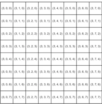
The most popular technique to fragment geospatial data for road networks is Slippy tiles [13]. It is used by both Google Maps and its open source competitor OpenStreetMap. First of all the Mercator projection is used in order to have straight edges on the tiles. Next, each tile can be represented by a single 3-tuple (zoom, x, y) where x is the longitude, y is the latitude and zoom defines the size. An example of zoom level 3 tile numbers in a Slippy tile representation is shown in Figure 2.3. The zoom level can range from 0, i.e. one tile covering the whole world, up to 18 or more resulting in several billion tiles for the whole world. An example of a tile defining URI could be represented as:

http : //.../zoom/X/Y (2.1)