The Triptych approach revisited: A staged sectoral approach for climate mitigation

(1)

Netherlands Environmental Assessment Agency (MNP), P.O. Box 303, 3720 AH Bilthoven, the Netherlands; Tel: +31-30-274 274 5; Fax: +31-30-274 4479; www.mnp.nl/en

MNP Report 500114008/2007

The Triptych approach revisited

A staged sectoral approach for climate mitigation

M.G.J. den Elzen* N. Höhne** P.L. Lucas* S. Moltmann** T. Kuramochiv Contact:

Michel den Elzen

Global Sustainability and Climate (KMD)

MNP – Netherlands Environmental Assessment Agency Michel.den.Elzen@mnp.nl

This research was performed with the support of the Dutch Ministry of Housing, Spatial Planning and the Environment as part of the International Climate Change Policy Project (M/500114).

* MNP – Netherlands Environmental Assessment Agency, the Netherlands ** Ecofys, Germany

v

(2)

Parts of this publication may be reproduced, on condition of acknowledgement: 'Netherlands Environmental Assessment Agency, the title of the publication and year of publication.'

(3)

Acknowledgements

This study was performed within the framework of International Climate Change Policy Support project (M/500114 ‘Internationaal Klimaatbeleid’. We would like to thank our

colleagues, in particular Jos Olivier for an extensive review of the report, Jeroen Peters for data support and Detlef van Vuuren (MNP), Dian Phylipsen (Ecofys, United Kingdom) and Robert Janzic (Ecofys, the Netherlands) for their contributions to the Triptych approach.

(4)

(5)

Rapport in het kort

De verbeterde Triptiek benadering

Een stadium, sectorale benadering voor toekomstige mitigatie verplichtingen

De Triptiek-benadering is een methode voor differentiatie van toekomstige verplichtingen tussen landen gebaseerd op technologische criteria op sectoraal niveau. De emissie- reductiedoelstellingen worden opgedeeld over de verschillende sectoren, waardoor het mogelijk is om dit te koppelen aan werkelijke reductiestrategieën. De nieuwe Triptiek 7.0 die hier wordt gepresenteerd is een verbetering ten opzichte van eerdere versies, vooral doordat het meer transparant is en het een vertraagde deelname toelaat voor de ontwikkelingslanden

(initiële deelname van de ontwikkelingslanden met een stimulans door ‘no lose’ doelstellingen of duurzame ontwikkeling beleidsmaatregelen). Dit rapport presenteert de emissie

reductiedoelstellingen van 224 landen voor drie scenario’s die broeikasgasconcentratie stabiliseren op 450, 550 en 650 ppm CO2-eq.. De reducties zijn ambitieus, maar verenigbaar

met bestaande technische reductiepotentiëlen.

Trefwoorden: Post-2012 regimes, sectorale doelstellingen, UNFCCC, toekomstige verplichtingen, technologie, emissies, klimaatveranderingen, broeikasgassen

(6)

(7)

Summary

How can an international agreement on climate change distribute responsibilities and emission reduction requirements between countries to be effective, technically feasible and is viewed as fair? This report further develops the Triptych approach as one possible answer to this

question.

The Triptych approach defines the criteria and rules for differentiating future commitments for all countries in a consistent and transparent manner. The advantage of the Triptych approach is that the rules to distribute emission allowances are different for each sector and are thereby linked to real-world emission reduction strategies. Its framework also allows for discussions on sectors that compete worldwide and, in a natural manner, on the role of developing countries in making contributions to emission limitation and reduction targets. The major downside of the approach, however, remains its complexity and the necessity for projections of production growth rates.

The Differentiated Convergence Triptych 7.0 presented in this report builds on an earlier version of the Triptych approach by refining the methodology to improve the transparency of the approach (e.g. a simplified methodology for the electricity sector) and to accommodate the tendency of developing countries to act only after industrialized countries have acted (initial participation of developing countries with incentives but no penalties through ‘no-lose’ targets or sustainable development policies and measures).

The approach has been implemented using a policy decision-support tool, the FAIR model, and the implications of the approach on the emission allowances of 224 countries are presented for the three sets of Triptych parameters – the slow, medium and strong scenario, respectively. The strong scenario is compatible with a stabilization of greenhouse gases (GHGs) at 450 ppm CO2-eq., and the medium scenario with a stabilization of GHGs at 550 ppm CO2-eq. All three

scenarios show that significant emission reductions are required for all regions. The reductions may sound very ambitious and (at first sight) politically unacceptable, but this study also shows that these are achievable in the short term with currently available technology and in the long term with very likely available technological options.

The modelling also clearly demonstrates that the very different emission profiles of countries can be considered in both an explicit and differentiated manner using the Triptych approach. The emission profiles of Brazil (dominated by agriculture) and China (dominated by use of coal) lead to different reduction requirements, because the Triptych methodology applies different rules for the different sectors.

We believe that even if the Triptych approach is not used as an officially recognized tool in its entirety during future negotiations, its elements constitute a useful input into such discussions and may eventually find an application in a definitive international climate agreement.

(10)

(11)

1 Introduction

The focus of attention in international climate negotiations has shifted from design of the specific rules of the first commitment period of the Kyoto Protocol (2008-2012) to

strengthening the international framework for the years following the Kyoto Protocol’s initial commitment period. At the eleventh Conference of the Parties (COP-11) in Montreal,

December 2005, countries agreed to start discussing the next steps to be taken, both under the Kyoto Protocol and under the United Nations Framework Convention on Climate Change (UNFCCC; see www.unfccc.int).

The long-term objective of the UNFCC (UNFCCC, 1992) is to stabilize the atmospheric greenhouse gas (GHG) concentration at a level that would avoid dangerous climate change impacts (Article 2). Consequently, the overriding challenge is to design an agreement that includes all of the major emitting countries – both developed and developing – and to

commence on taking the necessary steps to achieve significant long-term reductions of global emissions. To this end, many proposals for differentiating commitments among countries have been developed, including those developed by Parties to the UNFCCC as well as others

published in the literature (see Aldy et al., 2003; Blok et al., 2005; Bodansky, 2004; Kameyama, 2004; Torvanger and Godal, 2004 for an overview).

In this study, the global Triptych approach is developed further as a tool for allocating future emission allowances amongst countries within the framework of the international decision-making process on the differentiation of post-2012 commitments. The Triptych approach attempts to incorporate a number of widely supported notions in the climate debate, the most important of which are the necessity for technological improvement, the transition to low emissions and the desirability of reduction differences in per capita emissions. The Triptych approach assigns emission reduction commitments to individual countries according to

common rules using country-specific sector and technology information. These common rules allow for growth in economic activities (more for developing countries and less for developed countries) and require an improvement in efficiency or emission intensity. Although the Triptych approach is more sophisticated and, consequently, more data intensive than a number of other approaches (for example, those based on converging per capita emissions), these attributes provide it with the capability to take the diverse national circumstances of countries better into account.

The Triptych approach was originally developed at the University of Utrecht and has been used for supporting decision-making when differentiating the European Union’s (EU) internal Kyoto target among its Member States both before and after Kyoto (COP-3) (Blok et al., 1997; Phylipsen et al., 1998; Ringius, 1999). It may, therefore, serve the same purpose on a much broader international level.

The Original Triptych approach only comprised energy-related CO2 emissions and highlighted

(12)

industry),1_{(2) the domestic sector}2_{and (3) the electricity power sector. The initial selection of}

these categories was based on a number of differences in national and sectoral circumstances that were considered in the negotiations to be relevant to emission reduction potentials: differences in economic structure and the competitiveness of internationally oriented industries, in the standard of living and in the fuel mix for the generation of electricity. The emissions of the three categories are treated differently in that for each of the categories a reasonable emission allowance is calculated while at the same time relevant national and sectoral circumstances are taken into consideration. The methodology derives these allowances for each sector using uniform rules applied equally to all countries, and the sum of the

emissions allowances of the categories is the national allowance for each country. Only one national target per country is proposed – no sectoral targets – in order that countries be given more flexibility to pursue cost-effective emission reduction strategies.

In the years following the development of the Original Triptych, the approach was extended to the global scale and to include more sectors as well as non-CO2 GHGs (methane, CH4; nitrous

oxide, N2O; hydro fluorocarbons, HFCs; per fluorocarbons, PFCs; sulphur hexafluoride, SF6).3

The Global Convergence Triptych developed by Groenenberg et al. (2004) includes a target-oriented calculation scheme for calculating emission allowances from six sectors – fossil fuel production, agriculture and deforestation as well as the original three energy-using sectors – in which both CO2 and non-CO2 emissions are taken into account at the level of world regions.

The scheme defines global long-term sustainability targets for the GHG intensity of electricity production, for energy efficiency in the energy-intensive industry and for per capita emissions in the domestic sectors. Bottom-up data on sectoral reduction opportunities are used to set the level of the sustainability targets. The Global Convergence Triptych approach allows for a certain growth in activity in the various sectors and considers advanced technological opportunities to minimize their emissions. The level of growth activity allowed is based on medium growth projections for the various sectors. This Triptych approach has been used to review differentiation commitments for the 2010–2050 time frame.

A logical next step was to extend the calculation of the emission allowances to the level of countries, as individual countries are the actors in international negotiations and the emission profiles of countries may be very different even within one geographic region – for example, South Korea and China. Hence, individual countries are interested in the implications of various approaches for determining their emission levels. The Triptych 6.0 approach (Höhne et al., 2005) was the first attempt to extend the calculations to individual countries, and it

1_{Iron and steel, chemicals, pulp and paper, non-metallic minerals, non-ferrous metals and the energy}

transformation sector, including petroleum refining, the manufacture of solid fuels, coal mining, oil and gas extraction and any energy transformation other than electricity production.

2

The domestic sectors comprise various sectors: not only the residential sector (households), but also the

commercial sector, transportation, and light industry are included in this category, as are CO2 emissions related to

combustion in agriculture and during the production of fossil fuels.

(13)

incorporates two new elements in the methodology compared to the Global Convergence Triptych approach:

1. updated growth rates for the electricity and industrial production sectors combined with a ‘normative but scenario-derived’ approach or, stated otherwise, countries with low per capita income are allowed higher growth rates than in the default scenario, while countries with high per capita income are allowed lower growth rates than in the default scenario; 2. for the power sector, the emissions are based on assumptions for future shares of nuclear power and renewables and for changes in the fuel mix in fossil fuel-based power plants as well as for convergence in fossil fuel-based power generation efficiencies.

Furthermore, for the growth in the industrial production, Höhne et al. (2005) introduced a uniform ‘structural change factor’. This was a necessary adaptation since countries’ future industrial productivity data for the default scenario that accounts for structural changes were not available and, consequently, the economic indicator ‘industrial value added’ had to be used for future industrial productivity levels – and this indicator usually increases much faster than physical industrial production. The structural change factor converts the total ‘industrial value added’ into physical production growth of heavy industry. It therefore has a significant

influence on the results for the industry sector.

The methodology of the updated Triptych approach (‘Differentiated Convergence Triptych 7.0’, hereafter simply Triptych 7.0) presented in this study includes several other new elements that were added in response to the shortcomings of earlier implementations of the Triptych approaches:

 The calculation of the future emissions in the power sector assumes a growth in electricity consumption, an annual electricity consumption efficiency improvement (a decrease in demand), convergence of generation efficiencies per fuel and a decrease of the coal and oil shares in the electricity mix (for more details, see section 2.5). This methodology simplifies the calculation of emissions from the electricity sector compared to earlier versions and also solves some of the problems encountered using Triptych 6.0, such as the consideration of Combined Heat Power (CHP) or the implementation of shares of renewable and nuclear energy sources per country. The new methodology avoids the detailed estimation of efficiency improvements and conversion factors, and it leaves more freedom to countries in terms of how they would like to fulfil their share – with CO2-free energy by renewables, nuclear energy and CO2

capture and storage (CCS), or with low-CO2 energy (natural gas)

‘Common but differentiated responsibilities’ convergence, which means that all

convergence trajectories in the methodology are based on a ‘common convergence’, but are ‘differentiated’ in time. This translates into developing countries having the same obligation as developed countries to reduce emissions, but the obligation is delayed and conditional to the actions carried out by developed countries. This concept is based on the idea of Höhne et al. (2006a). Delayed participation of (least) developing countries

(14)

could overcome data implementation problems for these countries (for more details, see section 2.2).

Prior to participating in the convergence trajectories, developing countries commit in a clear and definite manner by adopting sustainable development objectives, the so-called Sustainable development policies and measures (SD-PAMs) or no-lose targets. For the implementation in the model, a uniform percentage reduction from baseline emissions for all sectors is assumed. The countries can decide whether they want to achieve this reduction with SD-PAMs or no-lose targets (for more details, see section 2.2).

The model implementation of the Triptych 7.0 approach in this report includes several other improvements compared to the earlier Triptych 6.0 version:

 The growth of industrial production is based on total final energy consumption in industry taken from the recently updated IMAGE 2.3 implementation of the International Panel on Climate Control Special Report on Emissions Scenarios

(Nakicenovic et al., 2000) (hereafter IMAGE 2.3 IPCC-SRES scenarios) (Van Vuuren et al., 2006a). As such, it also better accounts for structural changes in the industrial sector as well as autonomous baseline energy efficiency improvements compared to the earlier used growth in monetary value as “industrial value added” (for more details, see section 2.3 and Van Vuuren et al. (2006b)). This method is simpler and more coherent than that used in Triptych 6.0.

 Energy efficiency indices are based on national specific data, which are estimated in Triptych 7.0 for all individual countries based on the work of Kuramochi (2006) (for more details, see section 2.3). These indices are based on recent statistics data as compared to older and regional data applied at the level of countries used in Triptych 6.0 for the energy efficiency indices (from Groenenberg (2002)).

This report usesan updated baseline scenario of population, gross domestic product (GDP) and emissions at the level of 224 individual UN countries. This baseline scenario was derived from a downscaling methodology, based on the work of Van Vuuren et al. (2007), applied on the updated IMAGE 2.3 IPCC-SRES scenarios (Van Vuuren et al., 2006a) (for details, see section 2.1).4

The historical datasets of CO2 emissions at the level of all sectors has been updated

with the most recent estimates of the International Energy Agency (IEA, (2005a) and EDGAR datasets (Olivier et al., 2005) to 2003. The base-year for all other data, such as other GHGs, population, GDP, among others, remains 2000 (for more details, see section 2.1).

Note that both the renewed approach and Triptych 6.0 use the same definition of emission allowances, which is CO2-equivalent emissions, including the anthropogenic emissions of six

4_{Under Triptych 6.0, a set of baseline scenarios for population, GDP and sectoral emissions at the level of} countries, based on a linear downscaling method for the IMAGE 2.2 IPCC-SRES emission scenarios (Nakicenovic et al., 2000) was used. This methodology was highly criticized in the literature (see Den Elzen, 2005; Pitcher, 2004; Van Vuuren et al., 2007), as it may lead to unrealistic results.

(15)

Kyoto GHGs (fossil CO2, CH4, N2O, HFCs, PFCs and SF6 (using the 100-year GWPs of IPCC,

2001)) but excluding LULUCF (land-use and land-use change and forestry)-related CO2

emissions.5

This report is structured as follows. Chapter 2 describes the methodology of the updated Triptych approach, as implemented in our modelling framework, FAIR 2.1, at the level of individual countries (Den Elzen, 2005; Den Elzen and Lucas, 2005). Chapter 3 presents the emission allowances for three scenarios, including different convergence trajectories, and analyses whether these are compatible with achieving long-term GHG concentrations targets. Chapter 4 discusses the advantages and disadvantages of the Triptych approach and presents the main conclusions of this report.

5_{Emissions from LULUCF sources are highly uncertain, and emission estimates from various sources are often} not consistent. Therefore, it has also been suggested to treat emissions from deforestation with a different instrument separate from other emissions (WBGU, 2003).

(16)

(17)

2 Description of the Differentiated Convergence

Triptych 7.0 approach

This chapter describes the Triptych 7.0 approach in more detail. Table 1 presents an overview of the approach, the data requirements and the exogenous parameters that have to be chosen. Section 2.1 describes the modelling tool used for calculating countries’ emission allowances in the Triptych 7.0 approach. Section 2.2 describes the major new element of the Triptych 7.0 approach, the differentiated participation. Sections 2.3 to 2.7 describe the methodologies applied for the seven Triptych sectors – industry, electric power generation, domestic sector, non-combustion emissions from fossil fuel production, agriculture, waste and land-use CO2

emissions.

2.1 The modelling tool and data used

2.1.1 The FAIR world model

The FAIR 2.1 world model (Den Elzen, 2005; Den Elzen et al., 2007) is essentially a country-version of the FAIR 2.1 (region) model, which is a policy-decision support tool for analysing emission allowances and abatement costs at the level of 17 regions6_{(Den Elzen and Lucas,}

2003; 2005). The expansion of the model to the level of countries has been a major step

forward, and one that has only recently (2005) become possible as accurate and reliable data of baseline emission scenarios at the level of all world countries were not available prior to 2005, and downscaling methods have been the subject of criticism (see Den Elzen, 2005; see Pitcher, 2004; Van Vuuren et al., 2007) in that they have led to unrealistic results for some countries (in particular the one using the regional trend, as used by Gaffin et al., 2004; Höhne et al., 2003; Höhne et al., 2005). The model employed here uses a recently developed new downscaling method whose results are more reliable (Van Vuuren et al., 2007), as described below.

6_{More specifically, Canada, USA, OECD Europe, Eastern Europe, Former Soviet Union countries, Oceania and} Japan (Annex I regions); Central America, South America, Northern Africa, Western Africa, Eastern Africa, Southern Africa, Middle East & Turkey; South Asia (incl. India), East Asia (incl. China), South-East Asia (non-Annex I regions) (IMAGE-team, 2001).

(18)

Table 1 Main characteristics of the Triptych 7.0 approach.

Sector Approach selected Data needs User choices

General Definition

Target year 2010–2050 (2051–2100 are also calculated, but only for illustrative purposes) Annex I countries

emission level in 2010

- Kyoto countries: same share of sectors in 2010 as in baseline scenario - USA reaches its national target; Australia follows its baseline emissions.

Non-Annex I countries

Sustainable development policies and measures(SD-PAMs) or no-lose targets: before non-Annex I countries participate in the convergence trajectory (‘differentiated convergence’), they are committed to SD-PAMs or no-lose targets, which are

implemented in the model by a uniform percentage reduction for all sectors. More specifically, reduction below baseline linear increase from 1% in 2010 up to a maximum level in 2020, and constant afterwards (differs slightly among sectors; see section 2.2).

Maximum percentage reduction of baseline emissions

Kyoto GHGs CO2 , CH4, N2O, HFCs (sum), PFCs (sum) and SF6 • Excluding LULUCF CO2

emissions Countries Up to 224 (dependent on data availability)

Base-year emissions

The data are chosen as follows: (1) IEA data (CO2 emissions from fossil fuel combustion) (IEA,

2005a); (2) EDGAR data (www.mnp.nl\\/edgar) (CO2 (other than from fossil fuel combustion,

excluding LULUCF), CH4, N2O, HFC, PFC and SF6 emissions).

Baseline scenario IMAGE 2.3 IPCC scenarios A1B, A1f, A1T, A2, B1, and B2 are used consistently throughout the calculations, i.e. all required scenario elements are taken from the same scenario.

• Choice of scenario

Convergence year Starting of the convergence, convergence year and final reduction year differentiated for countries of four country groups (Box 1).

• Starting year • Convergence year • Final reduction year

Industry sector (‘Energy: Manufacturing Industries and Construction’ plus ‘Industrial processes’ as one sector (CO2,

CH4, N2O, HFCs, PFCs and SF6)

Growth rates of industrial production

The growth rates used are derived from the energy consumption in the industrial sector of the IMAGE 2.3 scenarios.

Industrial production growth rates for several sectors Energy efficiency Energy efficiency index (EEI) converges

to convergence level and subsequently further improves over time up to the EEI level in the reduction year.

Initial EEI for regions (taken from Kuramochi,(2006)

• EEI level in convergence year

• EEI level in reduction year

Domestic sectors (CO2, CH4 and N2O emissions from fossil fuel combustion from the residential, commercial, agriculture

and (inland) transport sectors and fluorinated GHG (F-gas) emissions from a range of sources (semi-conductors, refrigeration, air conditioning equipment, fire extinguishers and aerosol applications).

Convergence Linear convergence of per capita emissions

Population (UN, 2004)

• Convergence level

Annual reduction rate per capita domestic emissions after convergence

• Reduction rate after convergence

Power sector (CO2, CH4,N2O, HFCs, PFCs and SF6 emissions from electricity and heat production)

Production growth rates

The growth rates used are derived from the energy consumption in the power

Electricity demand derived from IMAGE

(19)

Sector Approach selected Data needs User choices

sector of the IMAGE 2.3 scenarios. 2.3 Method CO2 per kilowatt hour per fuel converges

to convergence level, and subsequently further improves over time up to the level in the reduction year.

Current emission factors and shares per fossil fuel type, from IEA (2005a)

• Convergence and reduction level of emissions factors per fossil fuels

Decrease of the shares of coal and oil in energy consumption

• Reduction of shares of coal and oil

Electricity end use efficiency improvements

• Annual electricity end use efficiency improvements

Fossil fuel production

Percentage reduction of baseline emissions in convergence and final reduction year

Baseline scenario emissions

• Reduction percentage in convergence and reduction year

Agriculture A technical, cost-effective emission reduction potential compared to the baseline scenario is assumed, accounting for activity growth and progress in animal and crop development. Different

reduction potentials for countries with lower income are applied compared to countries with higher income.

Baseline scenario emissions

• Reduction percentages compared to baseline scenario in convergence and reduction year for two groups of countries

Waste Linear convergence of per capita emissions to x tCO2-eq. per capita in

(differentiated) convergence year

Population • Reduction below base-year per capita emissions in convergence year

2.1.2 Data

For the historical data this report uses different data sources. The base-year (2000) population data are provided by the UN World Population Prospects (UN, 2004). The national per capita income levels in the base-year, expressed in purchasing power parity in U.S. dollars (PPP$),7

are based on the 2004 database World Development Indicators (WorldBank, 2004). The historical (1990–2003) sectoral countries’ GHG emissions (CO2, CH4, N2O, HFCs, PFCs and

SF6) are based on the IEA and EDGAR databases, i.e.:

1. CO2 emissions from fossil fuel combustion for the period 1990–2003 as

published by the International Energy Agency (IEA, 2005a);

2. CO2 (other than from fossil fuel combustion, excluding LULUCF CO2

emissions), CH4, N2O, HFC, PFC and SF6 emissions for the period 1990–2000

from the EDGAR database version 3.2 (Olivier et al., 2005).

The CO2 emissions from the IEA dataset were chosen, as this dataset is the most

comprehensive one available at the present time, and the emissions contained in it are

7_{The Purchase Power Parity (PPP) is an indicator of the GDP per capita and is based on the relative purchasing} power of local currencies in various regions, i.e. the value of a dollar in any country or, in other words, the dollars needed to buy a set of goods compared to the amount needed to buy the same set of goods in the USA.

(20)

calculated from official energy balances provided by the countries. This dataset does not include process CO2 and non-CO2 emissions,8 and the only global dataset available for these is

the EDGAR database (for the years 1990, 1995 and 2000). CO2 emissions from land-use

change are excluded in this analysis, but these could have been chosen from Houghton (2003). The emission sectors distinguished are:

Sectors IPCC EDGAR\IEA

Industry:

Industry (excluding coke ovens, refineries, etc.) Non-energy use and chemical feedstocks (CO2 only)

Iron and steel Non-ferro metals Chemicals

Solvent use/miscellaneous Pulp and paper

Cement production

HFC, PFC and SF6 use from a range of sources (semi-conductors,

industrial refrigeration and air conditioning equipment)

1A2 1A2 or 2B,C 2C1 2C3,5 2B 3 2D1 2A1 2F6, 2F1, 2F8, 2F2, 2F7, 2C, 2F6, 2C3, F10 F60 I10 I20 I30 I70 I50 I41 H11, H12, H14, H21, H24,H27, H28, H31, H35, H40, H45, H50, H55, H60 Electricity

Power generation (public and auto; including co-generation) Other transformation sector (refineries, coke ovens, gas works, etc.)

1A1a 1A1b,c

F20 F30 Domestic

Residential, commercials and other sectors (RCO) Transport road

Transport land road (rail, inland water, pipeline and non-specified)

HFC, PFC and SF6 use from a range of sources (domestic

refrigeration and air conditioning equipment, fire extinguishers, solvents and aerosol applications)

1A4 1A3b 1A3c,d-ii,e 2F3, 2F1, 2F4, 2F5, F40 F51 F54 H13, H22, H23, H25, H26

Fossil fuel production

Coal production+ (including CH4 recovery)

Oil production, transmission and handling Gas production and transmission

1B1 1B2a,c 1B2b F70 F80 (F81, F82, F83) F90 (F91, F92) Agriculture (non-energy related emissions)

Arable land (fertilizer use) Rice cultivation

Animals (enteric fermentation)

Animal waste management (confined N2O; all CH4); Animal waste

(deposited to soil - N2O)

Biomass burning Savannah burning

Indirect fertilizer/Indirect animal waste Biological N-fixation

Fuel wood burning

4D 4C 4A 4B 5A1, 4F 4E 4D 4D 5A2,3, 5B1 L10 L15 L20 L30, L60 L41, L43 L42 L75 L50 L44, L45 Waste (waste disposal and processing)

Landfills (including CH4 recovery)

Wastewater

Waste incineration (non-energy)

6A1,2 6B1,26B2 6C W10 W20, W30 (W39), W40 8_{Note that CO}

(21)

Emissions up to 2010 are estimated as follows:

It is assumed that Annex I countries (excluding the USA and Australia) implement their Kyoto targets by 2010, including those Annex I countries with baseline emissions in 2010 much less than their Kyoto targets, i.e. countries with excess emission allowances ( ‘hot air’).

It is assumed that the reductions necessary to meet the Kyoto target are achieved in all sectors equally: the sectoral reference emissions in 2010 are chosen and reduce

emissions of all sectors by the same factor so that the Kyoto targets are met. The years from the last available year up to 2010 are linearly interpolated. All Non-Annex I countries follow their baseline scenario up to 2010.

0 5000 10000 15000 20000 25000 30000 35000 Indus try Electricity Domes tic

Fos s il fuel production A griculture

W as te

Figure 1 Global GHG emissions of sectors in 2003 (in MtCO2) (excluding international aviation and marine bunkers

and land-use CO2 emissions).

For the future baseline emissions, the downscaling methodology of Van Vuuren et al. (2007) is applied on the updated IMAGE 2.3 IPCC-SRES scenarios, downscaling from the 17 world regions towards 224 countries. This report distinguishes the socio-economic driving forces of population size and per capita income levels as well as technological improvements, such as energy efficiency improvements and the type of fuels used, which is equitable to emission intensity (emissions per unit of GDP):

For downscaling of the population, the relative sizes of countries in the long-range population projections of the UN (2004) are used.

For downscaling per capita income and emission intensity (partial), convergence of the units to the average regional number is assumed, while ensuring that the total of the elements complies with the pathway of the larger unit.

For the energy- and industry-related sectors (industry sector, domestic sector, power sector and fossil fuel production), relative changes in the three components (population, per capita GDP and emission intensity) compared to the base-year (2000) are used to determine the future sectoral emissions per country.

(22)

For the agriculture and waste sectors, simple linear downscaling is used (regional emission trend for all countries within the region), as these sectors are only loosely linked to consumption and much more closely related to production levels.

2.2 Differentiated participation

In the Triptych 7.0 approach, convergence by ‘common but differentiated responsibilities’ is implemented. This means that all convergence trajectories in the methodology are based on a ‘common convergence’, but are ‘differentiated’ in time in that developing countries have the same obligation as developed countries to reduce emissions, but this obligation is delayed and conditional to the actions of the developed countries (Höhne et al., 2006a). More specifically, Annex I countries’ per capita emissions converge within, for example, 40 years (2010–2050) to a specific uniform per capita emissions level. Individual Non-Annex I countries’ per capita emissions also converge to the same level within, for example, 40 years, but starting when their per capita emissions are a certain percentage above the global average. Until that point is reached, Non-Annex I countries commit to policies and measures with a focus on their sustainable development objectives (Baumert and Winkler, 2005; Winkler et al., 2002)..

Two concerns often voiced in relation to the previous versions of the Triptych approach have been eliminated from Triptych 7.0. In the new Triptych 7.0 approach, developing countries are required to reduce emissions but in a delayed approach compared to Annex I countries; this condition is more compatible with the ‘common but differentiated responsibilities’ principle of the Climate Convention. The delayed participation also ensures that least developed countries are treated differently compared to the other countries, as a result of their delayed participation.

The calculations assume the following differentiated convergence of emissions for the developing countries: in accordance with the work of the South–North Dialogue Proposal of Ott et al. (2005), developing countries (i.e. Non-Annex I countries) are divided into four country groups on the basis of an index composed of indicators for responsibility (cumulative energy CO2 emissions/capita in the last decade), capability (GDP-PPP/capita) and potential to

mitigate (energy GHG emissions/GDP and GHG emissions/capita). These are (Box 1): 1. the newly industrialized countries (NICs; such as South Korea, Saudi Arabia,

Singapore);

2. the rapidly developing countries (RIDCs, such as Argentina, Brazil, China, Malaysia, Mexico, South Africa);

3. the other developing countries (Other DCs; such as like Egypt, India, Indonesia, Nigeria, Pakistan);

4. the least developing countries (LDCs; such as Afghanistan, Bangladesh, Tanzania, Zambia).

(23)

Box 1 Countries in different country groups (see Figure 2)

Newly Industrialized Countries (NICs): Bahrain, Brunei, Cuba, Israel, Kazakhstan, Korea (South),

Kuwait, Qatar, Saudi Arabia, Singapore, Suriname, Trinidad & Tobago, Turkmenistan, United Arab Emirates, Uzbekistan.

Rapidly Developing Countries (RIDCs): Algeria, Antigua & Barbuda, Argentina, Bahamas,

Barbados, Belize, Bosnia & Herzegovina, Botswana, Brazil, Chile, China, Colombia, Costa Rica, Cyprus, Dominican Republic, El Salvador, Fiji, Grenada, Guyana, Iran, Jordan, Lebanon, Malaysia, Malta, Mauritius, Mexico, Oman, Panama, Peru, Philippines, Saint Kitts & Nevis, Saint Lucia, Saint Vincent & Grenadines, South Africa, Thailand, Tunisia, Uruguay.

Other Developing Countries (DCs): Armenia, Azerbaijan, Bolivia, Cameroon, Congo, Cook Islands,

Ivory Coast , Dominica, Ecuador, Egypt, Gabon, Georgia, Ghana, Guatemala, Honduras, India, Indonesia, Jamaica, Kenya, Kyrgyzstan, Libya, Macedonia, Former Yugoslav Republic (FYR), Moldova, Mongolia, Morocco, Namibia, Nicaragua, Nigeria, Pakistan, Papua New Guinea, Paraguay, Seychelles, Sri Lanka, Swaziland, Syria, Tajikistan, Venezuela, Vietnam, Zimbabwe.

Least Developing Countries (LDCs): Afghanistan, Angola, Bangladesh, Benin, Bhutan, Burkina Faso,

Burundi, Cambodia, Cape Verde, Central African Republic, Chad, Comoros, Congo Dem. Republic , Djibouti, Equatorial Guinea, Eritrea, Ethiopia, Gambia, Guinea, Guinea-Bissau, Haiti, Kiribati, Laos, Lesotho, Liberia, Madagascar, Malawi, Maldives, Mali, Mauritania, Mozambique, Myanmar, Nepal, Niger, Rwanda, Samoa, Sao Tome & Principe, Senegal, Sierra Leone, Solomon Islands, Somalia, Sudan, Tanzania, Togo, Tuvalu, Uganda, Vanuatu, Yemen, Zambia.

Figure 2 Membership of countries in groups: Annex II countries, Annex II but no Annex I countries, NICs, RIDCs, other DCs and LDCs. Source: Ott et al. (2005).

(24)

For simplicity, this study assumes that the composition of the country groups does not change.9

The starting year of the convergence is now differentiated and defined in the scenarios

presented in Chapter 3 – for example, 2010 for the NICs, 2020 for the RIDCs, 2030 for Other DCs and 2040 for LDCs – while the convergence period for all countries remains the same. Prior to participation, the developing countries adopt SD-PAMs or no-lose targets, depending on their needs and their state of development.

In general, the SD-PAMs must be government actions that both have development and GHG emissions benefits (Winkler et al., 2002). SD-PAMs do not necessarily reduce emissions in absolute terms, as energy use and emissions in developing countries will need to grow to meet the requirement of sustainable economic development. Examples of SD-PAMs are improvements in energy and energy conservation and a switch to low carbon fuels, both of which provide sustainable development benefits in terms of energy security, reduced air pollution, higher employment levels and reduced costs for consumers and companies (Baumert and Winkler, 2005).

No-lose targets set a limit for total emissions in a target year. If this target is exceeded (real emissions are below the target), the additional emission allowances can be sold on the carbon market. If the target is not met (real emissions are above the target), no additional rights have to be bought. As such, no-lose targets are seen as an incentive for developing countries to participate in the system, but it is an option that requires an enhanced ability to quantify emission and emission reductions.

In the Triptych 7.0 approach, the reduction targets of the SD-PAMs and the no-lose targets are implemented as a national reduction factor compared to the reference case. Developing

countries will reduce their emissions by roughly 10% compared to their baseline emissions within the first 10 years after 2010; more specifically, the reduction below the baseline linear increases from 1% in 2010 to 10% in 2020, and remains at 10% thereafter. This is in line with the results of two other studies that analysed the impact of first reduction activities in

developing countries (Höhne and Moltmann, 2007; Ogonowski et al., 2006)and found these to be in the order of 10–15%. For all sectors except power and industry, this study assumes emission to be 10% below baseline emissions within 10 years. The power and industry sectors were treated differently since detailed data are necessary when countries participate at a later stage:

Power sector: the shares of energy sources in the year when the country participates are assumed to stay constant for the period 2004 until the differentiated starting year; emissions per kilowatt hour decrease by 1% per year over a 10-year period compared to baseline. This is roughly equivalent to a 10% emission reduction compared to the baseline in 10 years.

9_{Den Elzen (2005) and Den Elzen et al. (2007) analysed how the composition changes under the South-North} Dialogue proposal compatible with meeting different long-term greenhouse concentration targets.

(25)

Industry sector: efficiency improvements increase by 1% per year, which – over a 10 year period – is roughly equivalent to a 10% emission reduction compared to the baseline.

2.3 Industry sector

In the Triptych 7.0 approach the industrial sector consists of the manufacturing industry and construction. Due to the lack of available data, the industrial sector is handled in its entirety – i.e. energy-intensive and light industry are not treated differently.

The general concept is that the physical production of goods is growing while at the same time energy efficiency is improving. This study used the methodology of Groenenberg et al. (2004), but now with differentiated convergence.

Future production – The growth of industrial production is based on energy consumption in industry (excluding electricity) taken from the IMAGE 2.3 IPCC-SRES scenarios. In this way, Triptych 7.0 accounts better for structural changes in the industrial sector as well as for

autonomous baseline energy efficiency improvements, as described in detail in Van Vuuren et al. (2006b), compared to the earlier used growth in monetary value as “industrial value added”. If Western Europe is taken as an example, the total efficiency improvement for the IMAGE 2.3 B2 IPCC-SRES scenario (used for the default calculations) is 0.8% per year over the period 2000–2050, with 0.7% of this due to energy efficiency improvements and 0.1% due to structural changes. For China, the total improvement rate becomes as high as 6%, of which 2.5% derives from energy efficiency improvements.

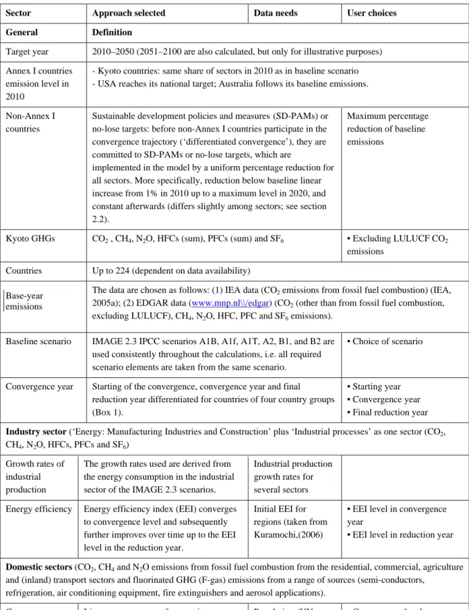
Energy intensity – For the energy-intensity levels, a worldwide convergence in energy efficiency levels of all countries over time is assumed (Groenenberg, 2002). A convenient indicator for energy efficiency is the EEI (Phylipsen et al., 1998). This index is defined as the ratio between the specific energy consumption (SEC) (energy consumption per tonne of product) for each region divided by the theoretical SEC using best current practices or best available technologies. For example, an EEI of 1.05 in a region means that the average SEC is 5% higher than the reference level, so that 5% of energy could be saved in the given sector structure10_{by implementing the best practice level technology. The SEC of a package of}

energy-intensive commodities is aggregated in the EEI, resulting in aggregated EEIs over the various subsectors in the energy-intensive industry for all countries, each representing a relative measure of the average efficiency of the energy-intensive industry in that specific country. For a further description of the EEI, see Appendix B. This study has used the recently updated values based on the work of Kuramochi (2006) and Höhne et al. (2006b) as

summarized in Table 3.

10_{The sector structure can be defined as being determined by the mix of activities or products within a sector. This} mix may well influence the reference-specific energy consumption level (Phylipsen et al., 1998).

(26)

Compared to the EEI data used in the earlier study of (Groenenberg, 2002), the EEI data for the iron and steel, pulp and paper, cement and petrochemical industry11_{have been updated for the}

years 2000–2003 with improved data coverage, while the petroleum refining subsectors are newly added. The aluminium subsector considered by Groenenberg is omitted due to the lack of up-to-date energy consumption data. Various energy data sources are used, while the

consistency of the data is carefully examined, as summarized in Table 2 (for further details, see Kuramochi (2006) and Höhne et al. (2006b)).

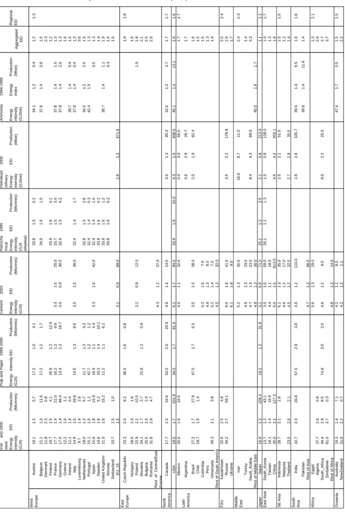
As an example, Figure 3 presents the EEI data for the sector iron and steel for the top 20 steel-producing countries. The numbers preceding the country names present the crude steel

production ranking in 2000. Among the top 20 producers, the EEIs ranged between 1.2 and 2.9, which means that the worst energy efficient country is nearly 2.5-fold less energy efficient than the best energy efficient country. South Korea can be seen to have the best EEI, 1.16, followed by Japan (1.2), France (1.4) and Germany (1.4). The EEIs for the remaining countries are given in Table 3. South Africa can be seen to have the lowest energy efficiency with an EEI of 2.9; other energy-inefficient countries with high EEIs include Russia, China and Poland.

Table 2. Sources used for the calculation of the Energy Efficiency Indices (EEIs) of Kuramochi (2006) and Höhne et al. (2006b).

Sector Production Energy

consumption

Best practice specific energy consumption (SEC)

Further details, see:

Iron and steel International Institute for Iron and Steel (IISI, 2005)

IEA’s Energy Balances (IEA, 2005c; 2005d)

Farla and Blok (2001); Kim and Worrell (2002)

Kuramochi (2006)

Pulp and paper Food and Agriculture Organization of the United Nations (FAOSTAT, 2006) Various national statistics, see Kuramochi (2006)

Farla et al. (1997) Kuramochi (2006)

Cement National statistics

and data from ENCI (2002)

Kim and Worrell (2002) Höhne et al. (2006b) Petrochemical industry Phylipsen et al. (2002) IEA’s Energy Balances (IEA, 2005c; 2005d)

Phylipsen et al. (2002) Phylipsen et al. (2002)

Petroleum refineries

Actual crude intake (IEA, 2005b)

Höhne et al. (2006b) Höhne et al. (2006b)

11

The designation Petrochemical industry refers to ethylene production, whereas the term petrochemical refineries refers to crude oil refining and cracking, which is a process to produce products from which ethylene is made.

(27)

Table 3. The EEIs at the country level. Source: Kuramochi (2006). Ir on and st e e l 2 000 P u lp a nd P ape r 199 9-20 00 C e m e n t 20 03 P e tr o c he mi c a l 19 95 P e tr ol e u m re fi ner y 2 000 A m m o ni a 1 994 -1 996 En e rg y in te n s it y (GJ/t) E E I P rod uc ti o n (Mt o n nes ) E n er gy in tens it y (GJ/ t) E E I P ro duc ti on (M to nne s ) E n er gy in te n s it y (G J /t) E E I P rodu c ti o n (M tonn es ) E n er gy in te n s it y (G J /t et hy lene ) E E I P rodu c ti o n (M tonn es ) E ner g y in tens it y (GJ/t o e ) E E I P rod uc ti o n (Mt o e ) E n er gy in te n s it y (G J /t o e ) E ner g y in d e x P rodu c ti o n (M to e) A ggr e gat ed EE I R e gi on al EE I We s t Eu ro p e A u s tr ia 19. 1 1 .5 5 .7 17. 2 1 .0 4. 1 3 3. 8 1 .5 0. 2 34. 1 1 .2 0. 4 1 .2 1. 3 B e lg iu m 21. 1 1 .5 11. 6 17. 2 1 .2 1. 7 3 4. 9 1 .6 1. 5 37. 8 1 .4 0. 8 1 .5 D e n m ar k 11. 8 2 .3 0 .8 2. 3 F in la n d 19. 7 1 .5 4 .1 26. 9 1 .2 12 .9 3 3 .8 1. 6 0 .1 1. 2 Fr anc e 17. 7 1 .4 21. 0 16. 2 1 .2 9. 6 3 .3 1. 0 20. 0 3 3. 7 1 .5 3. 0 37. 8 1 .4 1. 5 1 .3 G e rm a n y 17. 0 1 .4 46. 4 13. 4 1 .2 16 .7 3. 0 0 .9 30. 0 3 2. 9 1 .5 4. 2 37. 8 1 .4 2. 6 1 .3 G ree c e 12. 2 1 .6 1 .1 1. 6 Ir el an d 11. 1 1 .9 0 .4 38. 7 1 .4 0. 4 1 .5 It a ly 14. 9 1 .5 26. 8 14. 5 1 .3 8. 6 3 .5 1. 0 38. 0 3 2. 4 1 .4 1. 7 37. 8 1 .4 0. 4 1 .3 Lux e m bou rg 9 .7 1 .4 2 .6 3. 6 N e ther land s 18. 0 1 .2 5 .7 11. 7 1 .2 3. 3 3 2. 8 1 .5 2. 6 34. 0 1 .2 2. 5 1 .5 P o rt u gal 15. 1 1 .5 1 .1 42. 7 1 .2 1. 2 3 2. 4 1 .4 0. 3 42. 4 1 .5 1. 3 S pai n 15. 6 1 .8 15. 9 16. 9 1 .1 4. 4 3 .3 1. 0 42. 0 3 2. 4 1 .4 1. 0 0. 5 1 .3 S w e den 19. 6 1 .6 5 .2 33. 3 1 .4 10 .1 3 3 .8 1. 6 0 .2 1. 4 Un it ed K in gdo m 21. 0 1 .6 15. 2 11. 2 1 .1 6. 2 3 3. 8 1 .6 1. 2 38. 7 1 .4 1. 1 1 .9 No rw a y 33 .8 1 .6 0 .2 0. 3 1 .6 S w it z e rl an d 1 0 .7 1 .5 1. 0 1. 5 E U _1 5 1 .5 3. 1 0 .9 69. 0 2 .6 1. 2 671 .6 Ea s t Eu ro p e C z ec h R e p ubl ic 23. 3 2 .0 6 .2 36. 5 1 .6 0. 8 1. 9 1 .8 H ung ar y 18. 0 1 .5 1 .9 1. 5 P o la n d 22. 9 2 .1 10. 5 3 .2 0. 9 12. 0 1. 9 1 .8 S lova k ia 24. 1 1 .7 3 .7 22. 8 1 .2 0. 9 2. 1 B u lg ar ia 25. 5 2 .5 2 .0 2. 5 R o m ani a 31. 8 2 .8 4 .7 2. 8 Re s t of Ce nt ra l/ E a s t Eu ro p e 4. 3 1 .2 37. 0 No rt h Am e ri c a C ana da 17. 7 1 .5 16. 6 53. 5 2 .0 20 .9 4. 9 1 .4 14. 0 3 .5 1. 3 9 5. 3 32. 6 1 .2 3. 7 1 .7 1. 7 U S A 18. 5 1 .7 10 1. 8 34. 0 1 .7 81 .9 6. 1 1 .7 94. 0 3 3. 9 1 .6 10 .0 4 .3 1 .5 838 .5 40. 1 1 .4 1 3 .1 1. 6 1 .6 Me x ic o 20. 0 1 .6 15. 6 4 .0 1. 1 32. 0 5 .0 3. 0 6 6. 0 1 .7 1. 7 Lat in Am e ri c a A rg ent in a 4. 6 2 .9 26 .7 1 .7 B raz il 27. 2 1 .7 27. 9 47. 5 1 .7 6. 5 3 .5 1. 0 38. 0 2 .0 1. 9 8 2. 4 1 .6 Ch ile 18. 7 1 .5 1 .4 1. 5 Co lo m b ia 5. 2 1 .5 7 .0 1. 5 Pe ru 4. 9 1 .3 6 .0 1. 3 V e nez u e la 49. 3 2 .1 3 .8 5 .2 1. 4 7 .0 1. 9 Re s t o f S out h A m er ic a 4. 5 1 .2 32. 0 FS U K az ak hs ta n 32. 6 2 .5 4 .8 2. 5 2 .4 Ru s s ia 34. 2 2 .7 59. 1 6 .0 1. 8 41. 0 3 .5 2. 2 178 .8 2. 5 Uk ra in e 6. 1 1 .8 9 .0 1. 7 Mi dd le Ea s t Ira n 5. 2 1 .3 30. 0 16. 6 8 .7 1 1 .0 2. 4 2 .3 Tu rk ey 4. 9 1 .3 33. 0 1. 4 S aud i_ A rab ia 4. 7 1 .3 23. 0 8 .4 4. 3 8 9. 9 3 .3 Re s t o f Mi ddl e E a s t 4. 9 1 .3 30. 0 45. 5 1 .6 1. 7 Ja p an Ja p an 16. 6 1 .2 10 6. 4 19. 2 1 .2 31 .8 3. 1 0 .9 71. 0 2 5. 1 1 .2 2. 5 2 .1 0. 8 213 .9 1. 1 1 .1 E a s t Asi a So u th _ K o re a 13. 7 1 .2 43. 1 3 .5 1. 0 59. 0 2 6. 1 1 .2 1. 3 1 .5 0. 8 128 .0 1. 0 1 .7 T a iw a n 18. 1 1 .4 16. 9 4 .4 1. 1 18. 0 1. 3 C h in a 35. 0 2 .1 12 7. 2 5 .0 1. 5 8 1 3 .0 4 .5 4 .2 203 .1 1. 9 S E A s ia Indo nes ia 28. 7 2 .1 2 .8 5 .1 1. 3 35. 0 2 .5 2. 1 5 1. 5 1 .5 1. 5 Mal a y s ia 4. 6 1 .2 17. 0 1. 2 T h a ila n d 23. 5 2 .6 2 .1 4 .5 1. 2 32. 0 2 .7 1. 8 3 5. 6 1 .4 S o ut h As ia In di a 32. 7 2 .0 26. 9 57. 5 2 .9 3. 8 4 .6 1. 2 1 1 0 .0 2 .8 2 .8 105 .7 39. 6 1 .4 9. 5 1 .6 1. 6 P a ki st a n 39. 6 1 .4 1 1 .6 1. 4 Re st of Asi a 4. 7 1 .2 66. 0 Af ri c a E gy p t 5. 6 1 .3 29. 0 1. 3 2 .1 A lger ia 37. 7 2 .6 0 .8 2. 6 S o u th _ A fr ic a 44. 4 2 .9 8 .5 74. 8 3 .0 2. 0 4 .6 1. 2 9 .0 8 .0 2 .2 2 5 .5 2. 7 Zi m bab w e 61. 0 3 .7 0 .3 3. 7 Re st o f Af ri ca 4. 8 1 .2 14. 0 Oc ean ia A u s tr a lia 24. 3 1 .4 7 .1 4 .2 1. 2 8 .0 47. 4 1 .7 0. 5 1 .5 1. 5 Ne w Z eal an d 31. 6 2 .2 0 .7 4 .2 1. 2 1 .1 2. 2

(28)

0.0 0.3 0.5 0.8 1.0 1.3 1.5 1.8 2.0 2.3 2.5 2.8 3.0 6. S outh K orea 2. J apan 11. F ranc e 5. Ge rma ny 12. Ta iwan 10. It aly 13. Ca nada 18. Be lgiu m 15. M exico_16. U K 8. Br azil 3. U SA 14. Sp ain 9. In dia 19. Pol and 1. C hina 4. R ussia 20. S outh A frica EEI

Figure 3 Energy Efficiency Indices (EEI) of the top 20 steel producing countries for year 2000, including secondary steel making in electric furnaces. Source: Kuramochi (2006).

It is very possible that some subsectoral EEIs in Table 3 have values below 1 (for example, for the cement sector for Japan) through the application of non-conventional technologies with significantly low SECs. The aggregated EEI of the regions ranges between 1.1 (Japan) and 2.4 (Russia). Due to an improved coverage of the industrial energy consumption, the regional aggregated EEIs for some regions have significantly changes from those reported by

Groenenberg (2002) (Table 4). The results of Kuramochi (2006) indicate larger differences in regional industrial energy efficiencies.

Table 4 Comparison of aggregated EEIs in the energy intensive industry of the regions.

Region EEI – Groenenberg (2002) EEI – Kuramochi (2006)

Canada 1.3 1.7 USA 1.7 1.6 Latin America 1.5 1.7 Africa 1.6 2.1 Western Europe 1.2 1.3 Eastern Europe 1.7 1.8 Russia 2.0 2.4 Middle East 1.6 2.3 South Asia 1.7 1.6 East Asia 1.9 1.7 South-East Asia 1.6 1.5 Oceania 1.7 1.5 Japan 1.3 1.1

The Triptych 7.0 methodology assumes that the EEI converges linearly to a convergence level in a given year of convergence. This convergence is differentiated for the different country groups, as described in section 2.2, with the same starting year for countries within the four

(29)

country groups (Box 1) and a common convergence period for all countries. This common level then decreases further as time progresses.

The methodology of considering energy intensity in industry includes the incorporation of future changes in energy consumption due to technological progress or energy saving, or structural changes in the industrial sector. Changes in the emission intensity of energy due to, for example, a fuel switch, technological changes or carbon capture and storage are not included. These effects would be small in the short term but could be large in the long term.

2.4 Domestic sector

The domestic sector includes fossil fuel combustion from the residential, commercial, agriculture and (inland) transport sectors and F-gases emissions from a range of sources (refrigeration, air conditioning equipment, fire extinguishers and aerosol applications). It does not include emissions from electricity used in these sectors. The allowable GHG emissions in the domestic sectors are assumed to be primarily related to population size, since they are determined by the number of people in dwellings and at workplaces and by those needing transport, etc. Therefore, it is assumed that the GHG emissions per capita will converge differentiated (same starting years for the four groups of developing countries as described before) and linearly to the same level worldwide over the same period (e.g., 40 years). This level includes a convergence of the standard of living (e.g. number of cars, fuel use per household for space heating) and a reduction in existing differences in energy efficiency of buildings and vehicles. Groenenberg (2002) uses a medium value of 2.0 tCO2-eq. per capita in

2050, with a range of 1.5 to 3.0 tCO2-eq. per capita. Total emissions in the domestic sector are

determined by multiplying the per-capita emissions for each year with the population for that year, according to the reference scenario.

2.5 Power sector

The electricity -production sector is treated separately because specific GHG emissions from power production vary to a large extent among countries due to large differences in their shares of nuclear power and renewables and in the fuel mix in fossil fuel-fired power plants. The potential for cutting GHG emissions arising in this sector differs accordingly. Therefore, the fuel mix in power generation is an important national characteristic to take into account in the differentiation of commitments.

The calculations of the future emissions in the power sector assume a growth in electricity consumption (from the IMAGE baseline), a convergence of emissions per kilowatt hour per fuel, a decrease in the coal and oil shares in the fuel mix, an improvement in the efficiency of electricity consumption and a decrease in electricity consumption (demand) of the industry and domestic sector. The last four aspects are the same for all countries:

(30)

1. Convergence of emissions per kilowatt hour per fuel: The emissions per fuel converge (in CO2 per kilowatt hour) for each fuel by a differentiated year (see Table 5).

2. Decrease in the share of coal and oil in the fuel mix: The share of coal and oil in the mix of fuels used decrease linearly compared to the 2004 levels (for example, by 30% until 2030 and by 75% until 2050). A major proportion of this reduction can be achieved by CCS, in particular for the meeting the stringent climate targets, and by renewables. Accordingly, countries with high shares of coal and oil power stations need to reduce to a greater extent than counties which currently have a low share.

3. Annual improvements in the efficiency of electricity consumption (compared to the baseline electricity consumption): This is due to their convergence trajectories (for example, by 1.5% per year) (see section 3.2). This factor of decreasing demand from the industry and domestic sector is also included in the Global Convergence Triptych approach developed by Groenenberg et al. (2004).

The following formula illustrates how emission reductions are calculated in the first reduction phase for Annex I countries for the year 2030 under the strong scenario with a 1.5% decrease in electricity consumption and a 60% reduction in the share of coal and oil (compared to 2004 levels):

(

)

) kWh CO g 300 consum elec. %) 60 1 ( kWh CO g 450 consum elec. %) 60 1 ( kWh CO g 600 consum elec. ( % 5 . 1 1 consum elec. consum elec. emissions CO 2 2004 gas 2 2004 oil 2 2004 coal ) 2004 2030 ( 2004 total 2030 total 2030 AnnexI 2 × + − × × + − × × × − × = −

Applying these requirements and assumptions on the growth in electricity consumption, we are able to calculate the emissions that represent the limits of that specific country. For the

developing countries, the same formula is applied, but again with a differentiated convergence – that is to say, the same starting years for the four country groups (such as 2020 instead of 2004) and the same convergence period for all countries (as described in section 2.2) The approach as described above does not take into account heat production, which also contributes to emissions. According to the IEA (2005b), more than half of the power

production of some countries is based on CHP. The most notable of these are the Nordic and Eastern European countries, including Denmark, Hungary, Iceland, the Netherlands, Norway, Poland, Slovak Republic, Albania, Azerbaijan, Belarus, Kazakhstan, Kyrgyzstan, Latvia, Lithuania, Russia, Tajikistan and Turkmenistan.

Accordingly, this study considers emissions from the power sector to be the sum of the emissions from electricity production, as described in the formula above, and an adjustment factor (for heat production and other statistical differences between the datasets). For future

(31)

years, this adjustment factor declines at the same rate as the emissions from electricity production.

2.6 Fossil fuel production

Methane emissions from coal mining and from oil and gas production and distribution amounts to only about 5% of the total (2000) global GHG emissions; however, currently available technology can reduce this amount by around 60% compared to baseline levels in 2010 (Delhotal et al., 2006) and by up to 90% towards the end of the century. Therefore, as

emissions from this sector can be reduced drastically, emissions from fossil fuel production are treated as a separate sector. The baseline emissions from this sector are assumed to be scaled with the ratio baseline emissions and Triptych emissions from the three energy-consuming sectors. An additional reduction factor further reduces the emissions so that its reduction target can be reached in a (differentiated) convergence year (for example, 70% in 2050), with the reduction continuing until it reaches its maximum for a certain year (Lucas et al., 2007)

2.7 Agriculture sector

The emissions from the agricultural sector are expected to grow substantially, mainly in accordance with population and economic growth. However, substantial emission reduction options are available at relatively moderate costs (Graus et al., 2004). Under low concentration stabilization targets, reductions as high as 50% below the baseline emissions can be reached in the OECD countries in 2050, while in the non-OECD countries a somewhat lower reduction is reached (Lucas et al., 2007). Hence, emissions are assumed to be (linearly) reduced by a certain percentage below the reference scenario in the convergence year (differentiated), following which the reduction continues until a reduction percentage in 2100 is reached. This reduction is based on Lucas et al. (2007). Two groups of countries are distinguished: Annex I countries have to reduce more than ADC and LDCs.

2.8 Waste

Emissions from waste are substantial, but many emission reduction options exist (e.g. capture of CH4 from landfills). Hence, these emissions are treated as a separate sector. Emissions from

the waste sector are assumed to converge to a per capita level in a (differentiated) convergence year. The latter is taken to be a fraction of the global per capita emissions in the base-year, using reduction potentials based on Lucas et al. (2007).

(32)

2.9 Land-use-related CO

2

emissions

Data on land-use change and forestry is difficult to estimate and to assess. Emissions from this sector are always surrounded with many uncertainties. Due to this, land-use change and forestry emissions are not included in the Triptych calculations for this report.

(33)

3 Model analysis of the Triptych approach

3.1 Baseline emissions

The baseline scenarios used in this study are based on the set of SRES scenarios developed by (Nakicenovic et al., 2000) which explores different possible pathways for GHG emissions on the basis of two major uncertainties: (1) the degree of globalization versus regionalization and (2) the degree of orientation on economic objectives versus an orientation on social and environmental objectives. The storylines of the SRES scenarios have recently been re-implemented into the IMAGE 2.3 model (Van Vuuren et al., 2006a). This study uses the IMAGE/TIMER 2.3 SRES B2 scenario (hereafter referred to simply as the IMAGE 2.3 IPCC B2 scenario), which is a medium scenario, as the central baseline scenario, while all six

IMAGE/TIMER 2.3 IPCC-SRES (IMAGE 2.3 IPCC) scenarios – A1b, A1f, A1t, A2, B1, B2 – are used to show the impacts of different baseline assumptions. For the central B2 baseline scenario, energy-sector CO2 emissions continue to rise for most of the century due to

increasing coal and gas use, peaking at 18 GtC in 2080 (making the scenario a medium–high baseline compared to those presented in existing literature). Total Kyoto GHG emissions also increase, that is from a current 10 GtC-eq. to 23 GtC-eq. in 2100. As a result, by 2100, the baseline reaches a CO2 concentration of about 730 ppm CO2 and a GHG concentration of

850 ppm CO2-eq.

3.2 Three technology-oriented scenarios

STRONG: Early convergence to high technology standards with a large coalition

Basic idea: Climate change is considered by all countries to be an urgent problem, which is to be coped with through the cooperation of countries in terms of strong technology transfer.

Main assumption: Early convergence to the present (2004) level of the best performing Annex I country (such as CO2 emissions per kilowatt hour per fuel type) in 2030,

followed by common convergence to the lowest technical sectoral target in 2050 for the Annex I countries and newly industrialized countries (NICs) (Box 1). The advanced developing countries (ADCs) follow the same convergence, but with a 5-year delay, and the least developing countries (LDCs) are given yet an additional 5-year delay.

MEDIUM: Medium convergence to high technology standards, and a delayed convergence for the developing countries

Basic idea: Climate change is considered to be an urgent problem, but there is only a slow technological transfer from industrialized to less developed countries.

(34)

Main assumption: Starting in 2010, Annex I countries and NICs implement a convergence trajectory to the present (2004) level of the best performing Annex I country in 2050. The ADCs implement the same convergence pathway, but with a 10-year delay, and the LDCs are given yet an additional 10-10-year delay.

SLOW: Slow convergence to medium technology standards, and a delayed convergence for the developing countries

Basic idea: Climate change is not considered by all countries to be an urgent problem, and there is a slow technological transfer from industrialized to less developed

countries

Main assumption: Convergence to a target level that is about 10–15% above the present (2004) level of the best performing Annex I country in 2050, and then common

convergence to the lowest Annex I sectoral target in 2100. The NICs and ADCs do the same convergence, but with 10-year delay, and the LDCs are given yet an additional 10-year delay.

3.3 Choice of model parameters

A major element of the Triptych 7.0 approach is the differentiated convergence. The EEI in industry, the emissions per energy source in the power sector and the per capita emissions in the domestic sectors converge. The starting year of the convergence, the end year and a final year up to which the level is further reduced are chosen for the different country groups. Figure 4 provides an overview of these choices for the strong, medium and slow scenario,

respectively. The year 2010 is chosen as the simplified starting year following the first

commitment period of the Kyoto Protocol. At the same time, this is the starting year for further action for Annex I countries and NICs in the strong and medium scenario. For the slow

scenario, the NICs also enter the Triptych convergence, but 10 years later, in 2020. As

described above, the implementation of measures by ADCs and LDCs is delayed compared to 2010 by 5–10 years for the former and by 10–20 years for the latter. The convergence period for all countries is set at 20 years in the strong scenario and 40 years in the medium and slow scenarios.

(35)

90 95 00 70 75 80 85 50 55 60 65 30 35 40 45 10 15 20 25 Slow _ADCs LDCs LDCs AI NICs LDCs AI/NICs Str ong Medium AI/NICs ADCs ADCs

Convergence Reduction in all sectors Reduction in some sectors or of some

parameters

Figure 4 Starting of the convergence, convergence year and final reduction year for the scenarios and country groups, i.e. Annex I countries (AI), newly industrialized countries (NICs), advanced developing countries (ADCs) and least developing countries (LDCs) (see Box 1). The numbers at the top of the figure indicate year (2010, 2015, etc).

Table 5 presents the parameters chosen for the calculations in this report. Light-grey fields in the strong scenario include the convergence year or the respective parameter value. Medium-grey fields include the final convergence year or the respective parameter value, and dark-Medium-grey fields include (subsequent) reduction years or reduction values.

The sections below describe how the chosen parameters relate to what is possible, that is, the current status and possible future technological developments.

(36)

Table 5. Choice of model parameter for the three scenarios. Light-grey field indicates the (differentiated) convergence year and its convergence values, whereas the medium-grey field indicates the (differentiated) reduction year and its convergence year values. For the strong scenario, the dark-grey field indicates another final reduction year and the final reduction year values.

Sector Quantity Strong Medium Slow

General Overall effect of SD-PAMs and no-lose

targets: Reduction below baseline, linear increase from 1% in 2010 up to a maximum level (given in Table ?) in 2020, and a constant level thereafter (differs slightly among sectors, see section 2.2)

Approx. -10% Approx. -10% Approx. -10%

Convergence year (first column) and final years (second and third column) for Annex I countries and NICs, with 2010 as the starting year.

Convergence years for ADCs and LDCs are given in Figure 4

2030 2050 2100 2050 2100 2050 2100

Industry Level of Energy Efficiency Indicator 1.0 0.5 0.25 0.7 0.6 1.1 0.9

Domestic Domestic convergence level – per capita

emissions in tCO2 per capita per year

1.25 1.5 2.0

2% 1.5% 1%

Power Convergence (left) and reduction level

(right) of GHG emissions (gCO2/kWh)

Coal 600 400 200 600 400 700 600

Oil 450 300 150 450 300 500 450

Gas 300 250 100 300 250 350 300

Reduction in the share of coal and oil 60% 90% 95% 90% 95% 40% 80%

Decreased electricity consumption (demand) by the industry and domestic sector

2% 1% 0.5%

Domestic Domestic convergence level – per capita

emissions in tCO2/capita/year

1.25 1.5 2.0

2% 1.5% 1%

Fossil fuel production

Percentage-reduction of baseline emissions in convergence and reduction year

90% 95% 90% 90% 80% 90%

Agriculture Reduction below baseline emissions in

convergence and reduction year

ADCs and LDCs 30% 50% 20% 30% 10% 20%

Annex I countries and NICs 40% 50% 40% 50% 30% 40%

Waste Reduction below base-year per capita

emissions from waste in convergence year

The Triptych approach revisited: A staged sectoral approach for climate mitigation