Exploration of prokaryotic DNA methylation using deep learning

EXPLORATION OF PROKARYOTIC

DNA METHYLATION USING DEEP

LEARNING

word count: 21 767

Gaetan De Waele

Promoter(s): Prof. Dr. Ir. Wim Van Criekinge, Prof. Dr. Ir. Gerben Menschaert

A dissertation submitted to Ghent University in partial fulfilment of the requirements for the degree of master in Bioinformatics: Bioscience Engineering.

Deze pagina is niet beschikbaar omdat ze persoonsgegevens bevat.

Universiteitsbibliotheek Gent, 2021.

This page is not available because it contains personal information.

Ghent University, Library, 2021.

PREFACE

This thesis marks the end of my years as a student. Reflecting back, I realize that I have always gotten the most enjoyment out of projects and assignments. I am glad to be able to say that this was no different for my thesis. One year ago, I did not yet know what this thesis would exactly entail, especially given its broad scope. This has allowed me to pursue and come up with my own ideas, which has taught me that knowledge in data science arises from a careful balance of research and trial-and-error. Trying to find this balance was perhaps the most useful lesson of all.

I want to thank everyone at UGent involved in this project. Prof. Dr. Ir. Wim Van Criekinge, for making this thesis a possibility. Prof. Dr. Ir. Gerben Menschaert and Prof. Dr. Willem Waegeman, for the help and insights along the way. Finally, I would like to thank Jim Clauwaert, for providing guidance, while also encouraging me to explore this research in the ways I envisioned. Your lasting enthusiasm has motivated me to push further.

There are two more persons that deserve a special word of gratitude. These two have shaped me to the person I am today and it is impossible for me to envision a day in my life without them. I am overjoyed thinking about what the coming years have in store, and it is because I know you two will be at my side, through both hardships and pleasures. Thanks Mom. Thanks Daria.

CONTENTS

Preface i

Contents v

List of abbreviations vii

Abstract (English) ix

Abstract (Dutch) xi

1 Literature review: DNA Methylation 1

1.1 Introduction . . . 1

1.2 R-M systems and orphan MTases . . . 1

1.3 Regulatory function . . . 4

1.4 DNA methylation profiling . . . 4

1.4.1 Early methods . . . 4

1.4.2 Single-molecule real-time sequencing . . . 5

1.4.3 Oxford nanopore sequencing . . . 7

1.5 Methylation motifs . . . 8

2 Literature review: Machine Learning 9 2.1 Introduction . . . 9

2.2 Machine learning fundamentals . . . 10

2.2.1 Learning . . . 10

2.2.2 Optimization . . . 11

2.2.3 Bias and variance . . . 12

2.2.4 Model evaluation . . . 14

2.3 Deep learning . . . 16

2.3.1 Architectures . . . 17

2.4 Machine learning in (epi)genomics . . . 24

2.4.1 Motif discovery and sequence clustering . . . 25

2.4.2 Sequence labeling . . . 26

3 Results 31 3.1 Aims . . . 31

3.2 SMRT methylation data . . . 32

3.3 Clustering of methylated sites into motifs . . . 33

3.3.1 Clustering algorithm . . . 33

3.3.2 Motif evaluation . . . 34

3.3.3 Ablation study . . . 37

3.4 Genome-wide supervised modeling of methylated sites . . . 40

3.4.1 Model assessment . . . 40

3.4.2 Model interpretation for position importance . . . 45

3.4.3 Model interpretation for motif retrieval . . . 48

3.4.4 Model interpretation beyond the methylation motif . . . 51

4 Discussion 55 4.1 Motif discovery . . . 55

4.2 Sequence labeling of methylated sites using deep learning . . . 57

4.3 Future work and open questions . . . 59

5 Methods 63 5.1 Hardware and frameworks . . . 63

5.2 Data . . . 63

5.3 Clustering of methylated sites into motifs . . . 64

5.4 Genome-wide modeling of methylated sites . . . 66

5.4.1 Model architecture and training . . . 66

5.4.2 Toy dataset experiment . . . 68

5.4.3 Permutation feature importance . . . 69

5.4.4 DeepLIFT . . . 70

Bibliography 71

Appendix C Models with deviating PFI patterns 87

Appendix D Selection of DeepLIFT clustering motifs 89

LIST OF ABBREVIATIONS

Adam Adaptive momentum

AUC Area under the curve

CNN Convolutional neural network

DL Deep learning

DNA Deoxyribonucleic acid

m4C 4-methylcytosine

m5C 5-methylcytosine

m6A 6-methyladenosine

ML Machine learning

MTase DNA methyltransferase

NLP Natural language processing

ONT Oxford nanopore technologies

PFM Position frequency matrix

PR Precision-recall

R-M Restriction-modification

REase Restriction endonuclease

ROC Receiver operating characteristic

SMRT Single-molecule real-time

TCN Temporal convolutional network

TGS Third generation sequencing

ABSTRACT (ENGLISH)

DNA methylation is the most commonly studied epigenetic phenomenon in prokaryotes. Re-cent advancements in third generation sequencing technologies have made it possible to characterize complete methylomes on an unprecedented scale. This has revealed the com-plexity of methylation motifs and their biological functions. In this dissertation, DNA methy-lation data is studied using deep learning techniques. This class of models has the potential to elucidate more complex patterns. A clustering-based methodology for motif discovery is developed. Using this method, adenine-rich patterns associated with DNA methylation are observed. Additionally, an architecture to predict methylation of nucleotides in a genome-wide manner is proposed. Using this model, the effects of noise in methylation data are estimated. It is shown that m4C methylation calls are subject to a higher amount of noise than m6A calls. The prediction model is interpreted to reveal which sequence elements influence DNA methylation the most.

ABSTRACT (DUTCH)

DNA methylatie is het meest bestudeerde epigenetisch fenomeen in prokaryoten. Recente ontwikkelingen in third generation sequencing technologieën hebben het mogelijk gemaakt om volledige methylomen op een ongekende schaal te karakteriseren. Dit heeft de com-plexiteit van methyleringsmotieven en hun biologische functies onthuld. In deze disser-tatie wordt DNA methylatie bestudeerd met behulp van deep learning technieken. Deze klasse van modellen heeft het potentieel om meer complexe patronen bloot te leggen. Er wordt een op clustering-gebaseerde methodologie voor het ontdekken van motieven on-twikkeld. Met deze methode worden adenine-rijke patronen in associatie met DNA methy-latie waargenomen. Daarnaast wordt een architectuur voorgesteld om methymethy-latie van nu-cleotiden te voorspellen op een genoombrede manier. Met behulp van dit model worden de effecten van ruis in methylatiedata ingeschat. Er wordt aangetoond dat datapunten voor m4C methylatie onderhevig zijn aan meer ruis dan m6A data. Het predictiemodel wordt geïnterpreteerd om te onthullen welke sequentie-elementen DNA methylatie het meest beïnvloeden.

LITERATURE REVIEW: DNA

METHYLATION

1.1 Introduction

The term epigenetics was first defined by Conrad Waddington as "the branch of biology that studies the causal interactions between genes and their products that bring the phe-notype into being" (Waddington, 1968). With advancements in genetics, this definition has evolved. Today, the field of epigenetics can be defined as the "study of changes in gene function that are heritable and do not entail a change in DNA sequence" (Dupont et al., 2009). Perhaps more intuitively, the field searches for explanations for the behavior of genes that cannot be explained by their sequence. Mechanisms such as DNA methyla-tion, histone modifications, and RNA interference are well-known examples of epigenetics (Huang, 2012).

In prokaryotes, the most commonly studied epigenetic phenomenon is DNA methylation, the addition of a methyl group ( – CH3) group to DNA nucleotides. Three types of DNA

methy-lations have been described in prokaryotes: 6-methyladenosine (m6A) — the most preva-lent form in prokaryotes, 4-methylcytosine (m4C), and 5-methylcytosine (m5C) (Korlach and Turner, 2012). Shown in Figure 1.1, the DNA is methylated by a DNA methyltransferase (MTase) enzyme. MTases transfer a methyl group from S-adenosyl-L-methionine (SAM) to the correct place on the nucleotide (Beaulaurier et al., 2019). The remainder of this chapter is structured as follows. Section 1.2 and 1.3 describe DNA methylation and its functions in prokaryotes. In Section 1.4, a more general overview of methylation profiling techniques is given. Finally, Section 1.5 discusses methylation motifs.

1.2 R-M systems and orphan MTases

The best-known association of DNA methylation in prokaryotes is with restriction-modification (R-M) systems. MTases most frequently occur as part of an R-M system alongside a

cog-1.2. R-M SYSTEMS AND ORPHAN MTASES Adenine SAM SAH m6A m4C m5C MTase SAM SAM SAH SAH Cytosine MTase MTase

Figure 1.1: DNA methylation types in prokaryotes. During DNA methylation, a

methylgroup is transfered from S-adenosyl-L-methionine (SAM) to the DNA, producing a methylated base and S-adenosyl-homocysteine (SAH). Every MTase carries out one type of DNA methylation. Consequently, multiple MTases are necessary to perform different methylation types in the same organism.

nate restriction endonuclease (REase) with the same DNA binding specificity (Loenen et al., 2014). The REase cleaves non-methylated foreign DNA while the MTase protects endoge-nous DNA by methylating the same sites that the REase would cleave (Blow et al., 2016). Consequently, R-M systems can be regarded as primitive immune systems that protect prokaryotes against bacteriophages. Studies have shown a 10- to 108-fold protection against foreign DNA due to the presence of R-M systems (Tock and Dryden, 2005). Some phages have evolved to evade this system by modification of their own DNA, resulting in a co-evolutionary arms race (Bickle and Krüger, 1993).

The role of R-M systems in prokaryotic defense, however, does not explain their non-uniform distribution in prokaryotes and their exceptional sequence specificity (Vasu and Nagaraja, 2013). This implies that R-M systems have other roles in prokaryotic organisms. For exam-ple, R-M systems have been implied to function as selfish genes, seeking to promote their own survival and increase their relative frequency (Naito et al., 1995). Furthermore, by differentiating own versus foreign DNA, R-M systems provide a barrier for horizontal gene transfer (Murray, 2002). Consequently, a mechanism for genetic isolation is maintained, aiding the maintenance of different species and their separate evolution (Jeltsch, 2003). For a more complete and detailed overview of the functions of R-M systems described in literature, the reader is referred to Vasu and Nagaraja (2013).

Four categories of R-M systems have been defined based on the protein subunits involved, the site of DNA restriction relative to the binding site of the R-M system, and the nature of the recognition sequence. Type I systems consist of a single protein complex performing both restriction and modification. The location of cleavage is usually hundreds of base pairs away from their bipartite recognition sequence. In contrast, type II R-M systems generally consist of a separate REase and MTase acting independently (Roberts et al., 2003). REases of this type usually cut at their site of recognition, which is generally short and palindromic. Type II REases are a frequently used tool in recombinant DNA technology because of their outstanding specificity and activity. As a consequence, most efforts to identify new R-M

5'-CC

A

TNNNNNNGTTT-3'

3'-GGTANNNNNNC

A

AA-5'

5'-G

A

TC-3'

3'-CT

A

G-5'

5'-C

A

GAG-3'

3'-GTCTC-5'

Type I

Type II Type III

Figure 1.2: Typical recognition sequences of R-M systems. The methylated

nu-cleotides are indicated in red. Type I systems recognize bipartite sequences, where N can be any nucleotide. Type II systems recognize short palindromic sequences and type III systems recognize short non-palindromic sequences. Type IV R-M systems are not listed because they cleave modified DNA and are therefore not expected to frequently methylate the host genome. Exceptions to these rules are R-M systems belonging to the subclass IIG, which recognize non-palindromic sequences typically longer than those recognized by Type III systems. Note that in the case of type III and type IIg recognition sequences, the DNA is per definition hemimethylated, as there is no valid recognition sequence on the other strand.

systems have been directed towards this type (Pingoud et al., 2014). Type III systems are heterotrimers or heterotetramers of restriction and methylation subunits. They cut at a close (~25bp) distance from their short asymmetric recognition sequences (Dryden et al., 2001). Typical sequence specificities of these types are illustrated in Figure 1.2. A

fourth type of R-M systems has been reported that, in contrast to the other types of R-M

systems, only cleave modified DNA. The sequence specificity of this type of R-M systems has not been well described yet (Vasu and Nagaraja, 2013). It should be noted that the classification of R-M into types and subtypes does not completely represent the complexity of R-M systems found in nature, as enzymes have been reported that could fall into more than one subdivision (Roberts et al., 2003).

Not all MTases work together with a cognate REase in an R-M system. These ’orphan’ MTases are increasingly found in the prokaryotic kingdom, and it is assumed that they derive from R-M systems that lost their restriction counterpart (Sánchez-Romero et al., 2015). Orphan MTases are most frequently type II MTases, methylating short palindromic sequences (Blow et al., 2016). The Dam MTase found in Gammaproteobacteria is perhaps the most exten-sively studied example of an orphan MTase. It methylates 5’-GATC-3’ sites in a highly pro-cessive manner not encountered in R-M systems (Cheng, 1995). Another well-documented orphan MTase is the cell-cycle regulated MTase (CcrM), identified as playing an essential cell function in certain Alphaproteobacteria (Collier, 2009).

The Restriction Enzyme Database (REBASE) collects all information reported in literature about R-M systems and orphan MTases. Importantly, it also provides information about sequence specificities and cleavage patterns (Roberts et al., 2010).

1.3. REGULATORY FUNCTION

1.3 Regulatory function

As mentioned above, DNA methylation adds a methyl group to DNA. This methyl group protrudes from the major groove of the double helix, a typical binding place of DNA binding proteins. Consequently, DNA methylation has been reported to regulate protein binding to DNA (Wion and Casadesús, 2006). This way, DNA methylation of a regulatory region, such as a promoter, can impact transcription (Casadesús and Low, 2006).

Two types of transcriptional regulation are reported in literature (Low and Casadesús, 2008).

Clock-like control systems exploit the fact that DNA becomes hemimethylated after

replication. During the period of lag when remethylation is not yet complete, genes can be differentially regulated. A chromosome replication gene has been found to be regulated in this way, signifying the effect of this type of regulation on cell cycles (Kücherer et al., 1986). Switch-like control systems, on the other hand, arise due to binding competition of MTases and other DNA binding proteins. This binding competition results in recognition sites that are not methylated, reminiscent of DNA methylation patterns found in eukary-otes (Sánchez-Romero et al., 2015). In contrast to eukaryeukary-otes, active DNA demethylation mechanisms are not yet identified in prokaryotes. Competitive binding of proteins is con-sequently the only mechanism to produce DNA methylation patterns where methylation is not complete (Casadesús and Low, 2006). Switch-like controls of DNA methylation play an important role in phase variation of prokaryotes (van der Woude, 2006).

In addition to its impact on cell cycle regulation and phase variation, DNA methylation has been illustrated to impact virulence (Heithoff et al., 1999), motility (Oshima et al., 2002), adhesion (Erova et al., 2006), and other biological processes (Heusipp et al., 2007).

1.4 DNA methylation profiling

Because the biological importance of DNA methylation in mammals has been recognized for more than half a century, most of the technological developments regarding detection of DNA methylation have been directed towards profiling m5C in eukaryotes (Razin and Riggs, 1980). Methods only profiling m5C do not provide a complete characterization of bacterial and archaeal methylomes, which also include m6A and m4C methylated sites. This section will discuss existing methods that are suitable to profile methylation in prokaryotes.

1.4.1 Early methods

Restriction enzyme-based mapping consists of analyzing the cutting sites of a

primar-ily determined by the sequence specificity of the MTase. Therefore, DNA can be digested with a methyl-sensitive restriction enzyme with the same specificity as the MTase. The pat-tern of cut and uncut restriction sites can then be analyzed with next-generation sequencing (NGS) to reveal which sites are methylated and which sites are not (Nelson et al., 1993). This technique is robust, reliable and accurate, but it requires that the MTase specificity is known. Therefore, it can only identify sites modified by that specific MTase. As a conse-quence, it is not suitable for discovering new motifs or generating complete methylomes (Beaulaurier et al., 2019).

In bisulfite sequencing-based mapping, bisulfite treatment of the DNA before sequenc-ing converts unmodified cytosine to uracil, while leavsequenc-ing m5C bases unaffected (Kahra-manoglou et al., 2012). It has been popularly applied in eukaryotes because of its high sensitivity and compatibility with NGS technologies, but its application in the prokaryotic kingdom is limited, owing to being unable to profile m4C and m6A modifications (Beaulau-rier et al., 2019). Recently, a bisulfite sequencing method to profile both m5C and m4C has been developed by Yu et al. (2015). The proposed method consists of oxidating m5C to 5-carboxylcytosine (ca5C) with an enzyme before bisulfite treatment, which is subsequently read as thymine by NGS technologies. This extra step makes it possible to distinguish a fraction of m4C bases (Beaulaurier et al., 2019). However, the adaptation of this method is still limited because of its inability to profile m6A.

1.4.2 Single-molecule real-time sequencing

Third-generation sequencing (TGS) technologies are characterized by their ability to deter-mine the nucleic acid sequence without having to perform an amplification step (Schadt et al., 2010). As a consequence, the modification signal is still present at sequencing time and can be extracted. TGS technologies therefore make it possible to directly detect the complete methylome in a high-throughput manner. Single-molecule real-time (SMRT) se-quencing, developed by Pacific Biosciences, is the first technology that has proven to be up to the task in this context (Beaulaurier et al., 2019).

In SMRT sequencing, fluorescently labeled deoxyribonucleoside triphosphates (dNTPs) are incorporated into the template strand of the sample by an immobilized DNA polymerase. Multiple of these reactions are observed in real-time as several DNA polymerases are each immobilized to the bottom of a zero-mode waveguide (ZMW), a nanophotonic well with a diameter smaller than the excitation light’s wavelength, causing illumination light intensity to decay exponentially (Flusberg et al., 2010). Consequently, as only the very bottom of the ZMWs are illuminated, background noise is reduced. Because every type of dNTP is labeled with a different fluorophore, incorporation of a nucleotide results in a fluorescence emission spectrum allowing differentiation between nucleotides and, therefore, sequence

1.4. DNA METHYLATION PROFILING

ZMW

A

B

Figure 1.3: A. Illustration of a zero-mode waveguide during the sequencing pro-cess. A ZMW contains exactly one immobilized DNA polymerase and catalyzes the

replica-tion of one SMRTbell template with the help of an adapter, pictured in purple. The SMRTbell template contains hairpin adapters illustrated in yellow and the DNA template to be se-quenced in blue. B. Fluorescent signal in time for two templates. Peaks are colored according to their respective emission wavelength, identifying the nucleotide. Larger inter-pulse durations are observed when a modification is present in the template, as illustrated in the upper plot. Image courtesy of Flusberg et al. (2010).

determination (Eid et al., 2009). For the DNA polymerase to be able to replicate the tem-plate DNA, the SMRTbell format is used. A SMRTbell temtem-plate is created by ligating hairpin adapters to both ends of the template DNA (as shown in Figure 1.3A). The hairpin adapters form a single-stranded portion to which an adapter can bind (Travers et al., 2010). The added advantage of this is the creation of a circular DNA molecule, which allows the DNA polymerase to sequence both strands multiple times as a single continuous long read. This allows the template sequence to be determined with greater accuracy. As the lifetime of the DNA polymerase is limited, a trade-off between template sequence length and consensus accuracy presents itself (van Dijk et al., 2018).

The time needed for a DNA polymerase to incorporate a nucleotide, defined as the in-terpulse duration (IPD), is dependent on modifications, making it possible to recognize methylated nucleotides by an aberrant rate of DNA synthesis, as shown in Figure 1.3B. The analysis of variation in polymerase kinetics, called kinetic variation, is used to statisti-cally determine if a modification is present (Flusberg et al., 2010). This kinetic analysis can be performed with a control experiment, where IPD values from native DNA are compared with IPD values from whole-genome amplified DNA containing no modifications. Control IPD values can also be predicted by a pretrained conditional random field model taking into account sequence context (Schadt et al., 2013). A simple t-test for every position then determines if the IPD value observed in the native DNA significantly differs from the IPD value distribution expected for non-modified DNA. A modified site will also affect IPD values up- and downstream of its position (Beaulaurier et al., 2019). The resulting kinetic signa-ture differs for the different types of methylation and is therefore used to call the type of modification at modified sites. In this manner, it is possible to reliably identify m6A and m4C starting from 25x coverage per strand. The modification present in m5C, however,

Cur rent Time A T C G A T C G A G T A A

B

Figure 1.4: A. Illustration of a nanopore (green) during the sequencing pro-cess using 2D chemistry. The motor enzyme indicated with the arrow ensures stepwise

translocation of the DNA, to which a hairpin adapter is ligated. The hairpin adapter, illus-trated in yellow, allows for subsequent sequencing of the complementary strand. B. The

current in function of time as the DNA template moves through the nanopore.

Note that a deviation from what is expected is observed in red when a methylation oc-curs. In this illustration, the methylation also affects the current for the next and previous nucleotide. In reality, the current will be affected for a larger context.

has no direct impact on base pairing, resulting in a more subtle effect on DNA polymerase kinetics (Clark et al., 2012). As a consequence, a minimum of 250x coverage per strand is necessary for the detection of this type of modification (Schadt et al., 2013).

1.4.3 Oxford nanopore sequencing

In Nanopore sequencing, developed by Oxford Nanopore Technologies (ONT), a protein nanopore is inserted into an electrically resistant polymeric membrane (Jain et al., 2016), across which a constant voltage is applied and measured by a sensor. On transloca-tion of single-stranded DNA or RNA through the nanopore, the electric current will form a "squiggle" pattern, illustrated in Figure 1.4B, dependent on the roughly 6 bases inside the nanopore. Because of this, 46 _{characteristic current levels exist, not accounting for}

possible modifications. This makes the basecalling procedure a challenging problem and a key factor determining accuracy (Wick et al., 2019). Most ONT basecallers are based on a neural network architecture consisting of gated recurrent units (Huang et al., 2019).

Library preparation includes the ligation of an adapter bound to a motor protein that en-sures stepwise translocation through the nanopore, and usage of tethering adapters that help localize templates to the nanopores (Beaulaurier et al., 2019). A hairpin adapter can optionally be ligated to allow for sequencing of the complementary strand after the tem-plate has been sequenced, improving consensus accuracy (shown in Figure 1.4A). This chemistry, called 2D, has largely been replaced recently in favor of the 1D2 chemistry, which tethers the complementary strand to the membrane instead, resulting in better read quality and sequencing speed (de Lannoy et al., 2017).

The ability to sequence single DNA molecules without an amplification step should tech-nically make it possible to detect modified bases with nanopore sequencing. However, existing methods are mostly limited to the detection of specific motifs or specific types of

1.5. METHYLATION MOTIFS

modifications (Xu and Seki, 2019). Efforts to create methods that generalize well to unseen motifs are based on the same statistical principles used in SMRT technologies, but are still limited in accuracy (Stoiber et al., 2016).

1.5 Methylation motifs

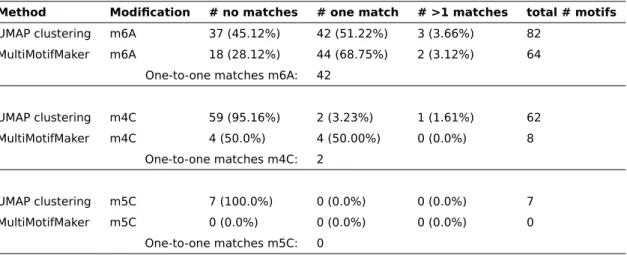
Mapping of methylated sites only provides limited biological insights into methylation mech-anisms. A more comprehensive characterization of the methylome requires discovery of the methylated motifs and corresponding MTases (Beaulaurier et al., 2019). A large di-versity in methylated motifs exists, as illustrated in Figure 1.2. It has been shown that differences in MTase sequence specificity within species result in different methylomes, transcriptomes and therefore phenotypes (Furuta et al., 2014), providing an explanation for the observed diversity in motifs. These motifs are usually represented as degenerate consensus sequences, using IUPAC nomenclature for positions where multiple bases can be present (Cornish-Bowden, 1985). This way, motif discovery can be cast as a combinato-rial optimization problem trying to find the most overrepresented nucleotide combinations. Specifically designed for methylation motif discovery, MultiMotifMaker uses a branch-and-bound algorithm to search the space of all possible motifs in conjunction with a scoring scheme that allows pruning of the search space (Li et al., 2018b). It returns all motifs that maximize Equation 1.1, where p represents the modification p-value associated with

a methylated instance  of the motif in question. The sum of the logarithms of all these p-values is multiplied with the fraction of motif instances in the genome that are methylated to produce a final score.

scor e(motƒ ) = Nmethyted Ntot N_{methyted} X ₌₁ og(p) (1.1)

Discovered motifs can be matched to an MTase by heterologous expression of the MTase in an organism devoid of MTases and observing which motif becomes methylated. Alter-natively, gene prediction tools can be used in conjunction with software suites such as SEQWARE (O’Connor et al., 2010), providing homology search tools for computational pre-diction of MTase domains (Blow et al., 2016). The sequence specificity of the MTase can then be predicted by comparison with closely related MTases with known specificity.

Mapping the methylome as well as motifs and MTases has proven to be the fundamental basis for further functional analyses to derive novel biological insights. Additionally, methy-lome data has shed light on the complexity and intricacy of DNA methylation in prokary-otes (Blow et al., 2016), motivating advanced modeling techniques to elucidate underlying mechanisms.

LITERATURE REVIEW: MACHINE

LEARNING

2.1 Introduction

Machine learning (ML) refers to the detection of patterns in data using computer algorithms (Shalev-Shwartz and Ben-David, 2014). A machine learning model achieves this without explicitly programmed instructions, but rather learns the relevant reasoning from data. Machine learning as a research field lies within the intersection of artificial intelligence and data science. It also overlaps with other fields such as statistics, in the sense that it often uses the same models. In statistics, the goal is generally to make an inference about the population based on modeling of the available sample data, whereas in ML, the same model would serve to extract patterns and often predict future samples.

Conventional ML models are limited in their capability to use data in their raw form, making careful feature selection a necessity (LeCun et al., 2015). Deep learning (DL) entails ML algorithms that show a hierarchical, layered abstraction of data representation (Najafabadi et al., 2015), allowing the features relevant for the task at hand to be learned by the model itself. This capability of representation learning has proven to be especially powerful in big data settings, where the capacity of deep learning methods is significantly higher than con-ventional ML methods. Deep learning research has exploded in recent years and has trans-formed many fields such as computer vision, natural language processing (NLP), robotics, and more. State-of-the-art models have even surpassed human-level performance in cer-tain complex tasks such as image classification (He et al., 2015) and competitive video gaming (Vinyals et al., 2019).

As high-throughput methods for biology have become more readily available and afford-able, biology has been transformed into a data-driven science (Perez-Riverol et al., 2019). In this era of big data, deep learning is proving increasingly an indispensable tool for bioinfor-maticians to infer relevant insights (Eraslan et al., 2019). The applicability of deep learning to biological data is only expected to improve as techniques get adapted to the domain.

2.2. MACHINE LEARNING FUNDAMENTALS

The following sections will further elaborate on machine learning fundamentals (Section 2.2), after which an overview of deep learning algorithms and techniques is given (Section 2.3). Finally, the application of ML to (epi)genomics is discussed in Section 2.4.

2.2 Machine learning fundamentals

2.2.1 Learning

Depending on the goals and used data, different types of learning can be distinguished. The three major types are supervised, unsupervised and reinforcement learning.

In supervised learning, a model is constructed with the prediction of one or more target variables in mind. For example, one may want to predict how a patient responds to a certain drug based on molecular markers. In this example, the molecular markers and drug response are called the features and output, respectively. Every sample  ∈Rp constitutes a vector [1, . . . , p], where every element corresponds to a specific feature of that sample.

The aim is to learn a function ƒ that will take input data X = {(1), . . . ,(n)_{} ∈}Rn_×p

, with n the number of samples and p the number of features, and is able to accurately produce an output Y = {y(1), . . . ,y(n)_{} ∈}Rn_×k

, with k the number of outputs. Labeled data samples, for which both X and Y are known, are necessary to do supervised learning. The supervision part lies in the fact that the labeled data will direct the learning of the model towards a function that best approximates it. A further distinction in this type of learning can be made depending on the nature of the output. In classification, the output is discrete, whereas in regression the output is continuous.

Unsupervised learning does not model a target variable, and hence does not require

labeled data. The goal is to extract information by finding structure and relationships be-tween samples and/or features in X. Unsupervised learning takes on many different shapes depending on the problem at hand; a typical example of unsupervised learning is cluster-ing. Clustering approaches try to group similar examples and are widely used in exploratory data mining. An example of the applications of clustering in biology is protein homology modeling, where homologous sequences are grouped into gene families. Dimensionality reduction is also a popular technique that can be described as unsupervised in almost all cases. Dimensionality reduction tries to reduce the number of input features by either se-lecting from the original set of variables or extracting new features altogether. It is used in data visualization and to avoid the curse of dimensionality.

In reinforcement learning, an objective is being optimized by letting a software agent interact with an environment and rewarding the agent based on the outcome of the inter-action. The software agent typically has parameters that determine how it interacts with

its environment. For example, the agent can be a chess bot with parameters that will de-termine its moves. The goal of the agent in this scenario can be to predict the move that will earn the biggest reward, for example winning. The most crucial aspects in this type of learning are the model that the agent works with and the exact way the reward is for-mulated and optimized. Reinforcement learning is currently mainly applied in robotics and game playing.

2.2.2 Optimization

The learning aspect of ML typically refers to the optimization of a loss function. Mathe-matical optimization consists of finding the inputs for a function that will give its minimal or maximal output. To illustrate, consider the supervised regression problem of fitting a second-order polynomial curve to a training dataset X ∈Rn×1 and corresponding Y ∈Rn×1. Fitting the curve y(, ) = P2

=0

 _{= }

0+ 1+ 22 to the data in this case means

finding the values of the parameters or weights 0, 1and 2 that minimize the error

be-tween the curve and observed data. A typical choice of loss function J() for this problem would be the mean squared error 1N

PN

₌₁(y()− y((),))2. In ML, this process is referred

to as training the model, the curve y(, ) being the model in this case. This example is illustrated in Figure 2.1.

The problem outlined above has a closed-form solution for finding the optimal parameter values. However, many ML algorithms are solved with iterative optimization strategies. These methods differ in whether they can be applied to convex or non-convex loss func-tions. In convex optimization, there is only one optimal solution, whereas in non-convex optimization, locally optimal solutions different from the global optimum may exist (Bottou et al., 2018). Gradient descent is one of the most popular convex optimization methods and widely adapted in deep learning (Ruder, 2016). It uses the first-order derivative (the gra-dient) of the loss function w.r.t. the parameters to find (locally) optimal parameter values. The negative of this gradient points to the direction in which the loss function decreases the steepest. By iteratively tweaking the parameters in the direction of the negative gradient, a solution is found for which the loss function is minimal.

=  − η∇_J() _(2.1)

Equation 2.1 describes the update step for gradient descent, with ∇J() the gradient of

the loss function w.r.t. the parameters . Note that the loss J() is not only dependent on , but also on the observed data X and Y. η is the learning rate that determines the step in the direction of the negative gradient. The value for η must be carefully chosen, as both values that are too small and too large will result in slower convergence. Additionally,

2.2. MACHINE LEARNING FUNDAMENTALS

gradient descent may even fail to converge when the value is chosen too large (Ruder, 2016).

Apart from the parameters learned from data, machine learning algorithms usually have hyperparameters that are defined before training. Examples of hyperparameters are the polynomial degree of the polynomial regression example and the learning rate of gradient descent. These hyperparameters can also be optimized for the problem at hand. For exam-ple, a dataset of higher complexity will benefit more from a larger polynomial degree than a simple dataset where a linear relation is observed. During hyperparameter optimization, the performance of the model is estimated with data not used during training, referred to as the generalization performance. This out-of-sample performance can be estimated by simply holding out a fraction of the samples, denoted as the validation set. Alterna-tively, cross-validation can be performed in order to obtain a more robust estimate of the generalization performance. In this case, multiple model instances are trained, each with a different portion of the samples as the validation set. Hyperparameter search schemes range in complexity from simple grid searches to probabilistic approaches such as Bayesian optimization and metaheuristics such as evolutionary algorithms (Bergstra et al., 2011).

2.2.3 Bias and variance

Bias and variance in machine learning models arise from their complexity relative to the modeling problem at hand. The bias error refers to erroneous model assumptions, resulting in missing some of the relations between input and output (underfitting). The variance error refers to the ability of a complex model to ’memorize’ training data and consequently fail to generalize well to unseen samples (overfitting) (Hastie et al., 2009). This principle is illustrated in Figure 2.1. The bias-variance tradeoff states that the generalization error is a sum of bias, variance, and irreducible error (Friedman, 1997). Since tackling bias and variance is one of the cornerstones of successful modeling, many techniques are available to analyze, as well as remedy, over- and underfitting. A simple way to diagnose potential bias and variance problems is by analyzing training and validation loss during and/or after training. A high training loss is indicative of underfitting, while a high test loss relative to the training loss is indicative of overfitting.

To tackle underfitting, a more complex model or better feature engineering should be ap-plied in order to better model the relations between input and output. An example of this is choosing a higher-order polynomial in the polynomial regression example. For non-convex models, other potential avenues are to increase training time to let the optimization al-gorithm converge or to choose another optimizer altogether. Tackling overfitting usually involves reducing model complexity or collecting more data. One technique to control overfitting is regularization, which introduces a penalty for parts of the parameter space

2

0

2

x

0

1

2

y

sampled data

with ground truth

2

0

2

x

2

_{degree polynomial}

2

0

2

x

8

_{degree polynomial}

Figure 2.1: Overfitting illustrated. Ten datapoints y subject to the function n( +

4) were generated for ten -values between [−3, 3] with even spacing. Random noise sampled from N (0, 0.5) was added to the y-values. In each subplot, the sampled data and ground truth n( + 4) are shown by blue dots and green curves, respectively. In the middle subplot, a fitted second-degree polynomial is shown in orange, corresponding closely to the ground truth. In the right-hand plot, an 8thdegree polynomial curve was fitted and shown in orange. This curve is sensitive to small variances in the data due to the introduced noise and is an example of overfitting.

where bad generalization is expected. Regularization fights overfitting in situations where complex models are being trained on datasets of limited size (Bishop, 2006). The most clas-sical examples of regularization are the L2 and L1 norms, both penalizing large parameter values. J() = Jor g() + λ||||2 2= Jor g() + λ p X j₌₁ 2 j J() = Jor g() + λ||||₁= Jor g() + λ p X j₌₁ |j| (2.2)

Equation 2.2 represents the loss function with L2 and L1 norms applied, respectively. Jor g()

is the unregularized loss, p the number of parameters and λ the hyperparameter control-ling the amount of regularization. By applying these norms, optimization will try to min-imize both the original loss function and the norm, resulting in smaller parameter values and a simpler model. Both L2 and L1 norms rely on the assumption that having smaller pa-rameter values will improve generalization, but differ in their interpretation. The L1 norm penalizes the sum of the absolute values of the parameters, resulting in a sparse solution where some weights will equal to zero. This induced sparsity improves the interpretability of the model by eliminating the effects of some features. The L2 or Euclidean norm shrinks parameter values asymptotically to zero and has the extra advantage of more stable op-timization. Both types of penalties are combined in elastic net regularization where the behavior is a hybrid between L1 and L2 regularization. The regularizer in this case is given by λ1P

p

j₌₁|j| + λ2

Pp

2.2. MACHINE LEARNING FUNDAMENTALS

These type of regularizers assume overfitting is a global phenomenon, occurring every-where parameters take on large values, but the degree of overfitting can vary in different regions of the parameter space (Caruana et al., 2001). In early stopping, no such assump-tions are made. The loss of a set held out from the training set (usually the validation set) is tracked during the training process. Training will decrease the loss on this set up until a cer-tain point. Once this point has passed, only training loss will decrease as the model starts overfitting. Early stopping stops optimization at this turning point to achieve regularization (Prechelt, 1998). This technique is especially popular in cases where training takes a long time, such as in training deep neural nets on big datasets. More specialized regularization techniques for deep learning models will be outlined in Section 2.3.2.

2.2.4 Model evaluation

Model evaluation consists of reporting the performance of the model according to one or more measures in an unbiased and correct way. To obtain an unbiased estimate of model performance, data not used in training or any other process (validation) should be used. Consequently, a three-way split of the original data is necessary to not only train and tune hyperparameters, but to also report performance in an objective manner (Bishop, 2006). Comparable to hyperparameter tuning, test performance can be computed from a single held-out test set or a cross-validation scheme.

The appropriate final performance measure is dependent on the problem at hand and will affect interpretation. For regression problems, a typical metric is the average of squared or absolute errors across all samples. The most popular choice is the mean squared error (MSE): MSE= 1 Ntest N_test X j₌₁ (y(j)− y((j),))2 _(2.3)

In classification problems, a typical starting point is the confusion matrix, shown for a binary setting in Table 2.1. In the confusion matrix, the model predictions versus the ground truth labels are tabulated. This way, a further distinction is made than simply ’correct’ and ’incorrect’, regardless of actually positive or negative. For example, a model can in practice be able to classify actual positive samples accurately, but fail to recognize negative samples reliably. From the confusion matrix, multiple metrics can be derived. The main ones are the accuracy T P+TN+FP+FNT P+TN , precision

T P T P+FP, recall T P T P+FN and specificity T N T N+FP.

The accuracy, being the fraction of predictions the classifier got right, is most often not satisfactory in imbalanced cases. In these cases, there are many more instances of one class in comparison to the other, and a high accuracy can be achieved by simply predicting

Table 2.1: A confusion matrix for binary classification. Labels predicted by the model

and true labels are presented in the columns and rows, respectively.

Predicted

1 (Positive) 0 (Negative)

Actual

1 (Positive) True Positive (TP) False Negative (FN)

0 (Negative) False Positive (FP) True Negative (TN)

the overrepresented class every time. The precision is how many of the predicted positives are actually positive and the recall corresponds to the fraction of actual positives that were correctly predicted. Since these metrics formulate performance explicitly in terms of true positives, they are most useful when the main interest is in this class. The F1 score is the

harmonic mean of the precision and recall 2·precson·recpr ecson_{+rec}, and is used in cases where both

metrics are important (Hastie et al., 2009).

Most classification models do not directly return a prediction, but a probability correspond-ing to the confidence of the model that a sample belongs to a certain class. In most ap-plications, the decision threshold is set at 0.5, but it can also be tweaked to give the best performance in function of a chosen metric. The receiver operating characteristic (ROC) curve is a plot of the recall (or true positive rate) in function of 1 − specificity (or false positive rate) for various threshold values. As the threshold is lowered, one expects that more positives are recovered (i.e. the recall improves), but also that more false positives creep through (i.e. the false positive rate increases as well). If a good distinction is made between positives and negatives, a high recall is possible for low false positive rates, result-ing in a steeply risresult-ing curve. Consequently, the area under the curve (AUC) can be used as a threshold-independent performance metric that can be interpreted as the probability that the prediction model ranks a positive sample higher than a negative sample. The precision and recall exhibit a similar trade-off property, and the area under their curve can similarly be used as an evaluation metric. Because the trade-off between precision and recall does not directly consider the true negatives, it is less useful in cases where correct classification of both classes is important (Davis and Goadrich, 2006). A fictional example of ROC and precision-recall curves is given in Figure 2.2.

In unsupervised learning settings, model performance evaluation is less straightforward and more case-specific. The performance of a clustering method, for example, is highly subjective and dependent on the expectations of the user. In a research setting, the per-formance of clustering algorithms is compared using external validation, which requires labels. External validation is not useful from a practical point-of-view, because labels are not usually available when doing clustering. In these cases, internal validation techniques can be used. These techniques are based on separation and cohesion metrics, which quan-tify how far or close elements of same and different clusters are, respectively (Palacio-Niño,

2.3. DEEP LEARNING

0.0 0.2 0.4 0.6 0.8 1.0 False positive rate

0.0 0.2 0.4 0.6 0.8 1.0 T rue p o si tive r a te ROC curve 0.0 0.2 0.4 0.6 0.8 1.0 Recall 0.0 0.2 0.4 0.6 0.8 1.0 Pr e ci si o n Precision-recall curve

Figure 2.2: Fictional examples of ROC and Precision-recall curves. The curves for

two fictional classifiers are shown in blue and green. Because the area under both curves is the largest for the classifier shown in blue, this classifier outperforms the classifier shown in green in terms of both ROC AUC and PR AUC.

2019). A popular example of such a metric is the Silhouette Coefficient, given for a single sample by Equation 2.4 (Rousseeuw, 1987). With () the mean distance between sample  and other samples in the same cluster, and b() the mean distance between sample  and samples in the next nearest cluster. The distance measure can be freely defined by the user. The coefficient s() exists for every sample and can be averaged over the dataset to obtain a single score.

s()=

b()_{− }()

m((), b()) (2.4)

2.3 Deep learning

Even though the "No free lunch" theorem states that there is no single model that works best for every problem, the focus in this thesis is mainly on deep learning models. To mo-tivate this choice, the advantages over traditional models in the context of (epi)genomics needs to be clarified first.

Conventional machine learning models need careful feature engineering, a process requir-ing time and domain expertise (LeCun et al., 2015). Deep learnrequir-ing models are able to utilize data in its raw form, because they automatically discover the useful features in hidden rep-resentations. For genomic sequences, this means that it is possible to use the sequence as input itself, instead of going through the process of creating features such as k-mer counts. Furthermore, the universal approximation theorem states that feed-forward neural networks can approximate any function, given some assumptions (Cybenko, 1989). The flipside of this capability to solve extremely complex problems is that deep learning models usually need a lot of data. The combination of this need for lots of data, large models to train, difficulties in optimization, and a lot of hyperparameters to tune effectively made

Figure 2.3: The computational graph of a single neuron with three inputs.

Ev-ery input feature  is represented as a node. The result of linear combination of  with

learnable weights  and added bias b is z, from which the activation  for that neuron is computed via the activation function ϕ. This activation is used as input for the next layer. In graphs of neural networks, a single node is used to represent the computation of  from



deep learning computationally infeasible until recently (Dean et al., 2018). Another disad-vantage is the complex mapping of the input w.r.t the output, resulting the model being a "black box", a problem that is addressed by the field of explainable AI (Gunning, 2017). The big data era in biology goes hand in hand with the deep learning revolution, as now deep learning techniques are increasingly becoming adapted to the domain. The following sections will focus on explaining popular deep learning model architectures and techniques used in DL modeling.

2.3.1 Architectures

Multilayer perceptrons (MLPs) are considered the quintessential supervised deep

learn-ing model architecture (Goodfellow et al., 2016). Like all other deep learnlearn-ing models, they consist of an input layer, one or more hidden layers capable of representation and feature learning, and an output layer. An example of a multilayer perceptron with two hidden layers is given in Figure 2.7A. In MLPs, information in every feature and information flow is repre-sented by nodes and edges, respectively. The network is called dense, or fully-connected, because all nodes from any layer are connected to all nodes in the next. An MLP is also called a feedforward neural network because information exclusively flows forward with no feedback connections. Information flows by linear combination of the features in the previ-ous layer and subsequent non-linear activation. The learnable parameters of this network are the weights of the linear combinations. The computational graph for a single neuron is illustrated in Figure 2.3.

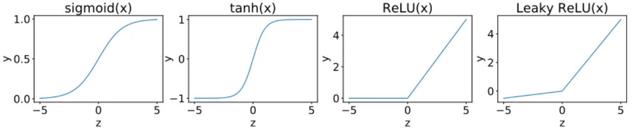
Since multilayer perceptrons without activation functions are nothing more than series of linear combinations, non-linear activation functions are necessary to learn non-linearities in the data. The sgmod activation function, given by Equation 2.5, is a differentiable function

2.3. DEEP LEARNING

5

0

5

z

0.0

0.5

1.0

y

sigmoid(x)

5

0

5

z

1

0

1

y

tanh(x)

5

0

5

z

0

2

4

y

ReLU(x)

5

0

5

z

0

2

4

y

Leaky ReLU(x)

Figure 2.4: Frequently used activation functions. Note the different y-axes for the

different subplots. A Leky ReLU = m(α · z, z) with α = 0.10 is illustrated here.

that maps its input to a value between 0 and 1 (Karlik and Olgac, 2011). It is particularly useful in output layers where the output needs to be interpreted as a probability.

σ(z) = 1

1 + e−z (2.5)

A similar activation function is the tnh function, given by Equation 2.6, which maps its input to a real number between -1 and 1. This has the effect of centering the means of the activations to zero, which has a beneficial effect on learning. The function is also steeper, making the derivatives larger and consequently promoting faster convergence (Kalman and Kwasny, 1992).

tnh(z) =

ez_{− e}−z

ez_{+ e−z} (2.6)

A major disadvantage of using a sgmod or tnh activation is the problem of vanishing gra-dients at large negative or positive input values. In these cases, the derivative approaches zero and learning slows down. The Rectified Linear Unit (ReLU), given by Equation 2.7, does not exhibit this problem and allows for more efficient computation of the gradients (Nair and Hinton, 2010). Different variations of the ReLU exist, of which the Leky ReLU is perhaps the best-known (Maas et al., 2013). The Leky ReLU has a small slope for neg-ative input values instead of a horizontal line. All of the previously mentioned activation functions are illustrated in Figure 2.4.

ReLU(z) = m(0, z) =    z _{if z > 0} 0 otherwise (2.7)

In the output layer, another frequently used activation function is the soƒ tm operation. This function uses the output layer vector as input and normalizes its values to sum to one. In this way, the output layer can be interpreted as a probability distribution. It is used in multi-class classification problems, where every sample is classified as belonging to one of more than two possible classes (Goodfellow et al., 2016).

soƒ tm(z) =

ez

P

je

zj (2.8)

It has to be noted that all previously mentioned activation functions are universally applied in all other deep learning architectures.

Convolutional neural networks (CNNs) are neural networks that use convolutions in at

least one of their layers (Goodfellow et al., 2016). In the context of CNNs, a convolution can be defined as a linear combination of locally-related features. More formally, it employs the computation of a sliding dot product of the input features and one or more learnable kernels. Equation 2.9 shows the mathematical formula in the most simple one-dimensional case, with a kernel k of length 2N + 1, where the asterisk denotes the cross-correlation operator. z= ( ∗ k)= N X j=−N +jkj (2.9)

In this equation, every output feature zis computed from a weighted sum of input feature

values _−Nuntil +N. The weights in this sum are determined by the kernel k. To illustrate

how convolutional layers produce an output, a simple example is shown in Figure 2.5. Addi-tionally, an example of a convolutional neural net for images is shown in Figure 2.7B. CNNs excel in finding relevant regularly appearing local patterns in data (Killoran et al., 2017). Consequently, they are frequently applied in fields such as computer vision and sequence modeling. It is important to note that convolutions can detect these patterns across mul-tiple channels. For example, in images, every pixel is characterized by three values for red, green and blue. The channels in the produced feature map correspond to the different patterns detected by the convolutional layer. The rationale is that more abstract, high-level representations are learned in deeper layers, allowing for classification.

Convolutional layers are usually combined with pooling layers, which merge features in or-der to reduce noise and extract meaningful signal while reducing spatial resolution (Rawat and Wang, 2017). A frequently-employed pooling operation is max-pooling, which only retains the largest activation from a set of adjacent inputs (Ranzato et al., 2007). Fur-thermore, how the input is convolved can be tuned with several hyperparameters such as padding, stride, and dilation.

Recurrent neural networks (RNNs) are neural networks that model sequence

depen-dency using a recurrent element that explicitly passes information in hidden layers from one element of the sequence to others, most frequently the next. In the simple case of a forward connection to the next element, the activations (T)of a hidden layer at an arbitrary time step T can be computed as shown in Equation 2.10. In this equation, the weight

ma-2.3. DEEP LEARNING

Figure 2.5: Illustration of a 1D convolution with kernel size 2 convolving over a 1D input sequence of length 4 with only 1 channel. In the case where more than one

input and/or output channel are involved, every and/or  contains a vector with multiple

dimensions. In this case, a kernel with separate weights is learned for each input/output channel combination. A separate bias is also learned for every separate output channel.

Figure 2.6: Illustration of an unrolled recurrent element for two time steps T and

T+ 1. The recurrent connections coming from and going to the illustrated time steps are

omitted from the figure.

trix W∈Rpot×pn linearly combines the input (T)∈Rpn×1 at a given time step to a vector

with the same amount of dimensions as the hidden state (pot). The matrix W∈Rpot×pot

linearly combines the activations from the previous time step. A visual representation of such a hidden layer is shown in Figure 2.6.

(T)= ϕ(W_(T−1)+ W_(T)+ b) _(2.10)

In RNNs, the weight matrices W and W are unique to each layer but are the same for all

different time steps. This way, RNNs are able to handle variable sequence lengths (Lipton et al., 2015). It is to be expected that this way, information from one time step quickly erodes as the next elements are processed. Consequently, RNNs are only able to capture relatively short-range dependencies well (Pascanu et al., 2013). The problem of long-range dependencies encountered in many sequence modeling problems has motivated research into alternative recurrent architectures, of which the long short-term memory (LSTM) archi-tecture is the most popular (Hochreiter and Schmidhuber, 1997). In many sequence mod-eling problems, forward dependencies between time steps also need to be accounted for. For this reason, bidirectional RNNs were introduced (Schuster and Paliwal, 1997). Whereas

Bias Bias Bias 1 1 1 Con v Con v Pool

Pool FlattenDense

Encoder

Decoder

A

B

C

D

Figure 2.7: Examples of all discussed architectures. Inputs and outputs are shown in

green and red, respectively. A. An MLP using only dense layers. B. A CNN using convolu-tional and pooling layers, as well as a dense layer at the end to produce an output. C. An RNN with two recurrent hidden layers. D. An autoencoder, the network is trained to output its own input. The encoder and decoder can be any sort of neural network architecture.

MLPs are used to produce one output of fixed size per input of fixed size, RNNs can also be used in scenarios where variable length inputs predict variable length outputs. Exam-ples are image generation from text (many-to-one), image captioning (one-to-many) and sequence labeling (many-to-many). The sequence labeling example is illustrated in Figure 2.7C.

All previously described architectures can be seen as encoders, which find patterns in data to produce a useful representation that is subsequently used for prediction. Decoders, on the other hand, use encoded representations to produce higher dimensional output. An

autoencoder, shown in Figure 2.7D, is an encoder-decoder pair that tries to reconstruct

its own input. After encoding the input to a low-dimensional latent space, it is to be ex-pected that not all information can be conserved, consequently resulting in an approximate reconstruction. This way, the learned representation will only capture the most important patterns in the data and remove noise. They are frequently applied for feature learning, dimensionality reduction, and, more recently, generative modeling (Dong et al., 2018).

2.3.2 Deep learning techniques

2.3. DEEP LEARNING

To train a neural network, gradient-based techniques are usually employed to update the parameters in order to optimize a loss function. In deep neural networks, where the gradi-ents for potentially millions of parameters need to be efficiently calculated, the backpropa-gation algorithm is used (Rumelhart et al., 1986). Backpropabackpropa-gation computes gradients by utilizing the chain rule as it iterates backward through the computational graph, determined by the model. State-of-the-art deep learning libraries provide automatic differentiation us-ing backpropagation (Ruder, 2016). A frequently-encountered problem with backpropaga-tion through deep neural networks is vanishing gradients. To help remediate this, residual connections can be used (He et al., 2016). Residual connections skip layers, for example by passing activations through a shortcut to the next but one layer. In this way, signal from one layer can be propagated deeper without going through activation, consequently helping to remedy the problem with vanishing gradients.

Because of optimization landscapes with multiple local optima, the gradient descent tech-nique outlined in Section 2.2.2 is often not satisfactory in the context of deep learning models. Mini-batch gradient descent is an alternative where, in each step, a subset of the training data is used (Bottou, 2012). Mini-batch gradient descent is necessary when big datasets are used where it is not computationally feasible to calculate the gradient for the whole dataset at once. Moreover, by approximating the gradients using only a small batch size, it is possible to escape local optima.

Momentum and adaptive learning rates are two popular additions to gradient-based op-timizers (Ruder, 2016). Momentum aids faster convergence by adding a fraction of the update vector of the past time step to the current update vector, whereas adaptive learn-ing rates aim to choose the learnlearn-ing rate of each parameter by taklearn-ing previous gradients of those parameters into account when calculating the update vector. Adam (adaptive momentum) is a proven optimizer implementing both principles (Kingma and Ba, 2014).

Improving generalization

Despite the large capacity of deep neural nets due to the large number of parameters, over-parameterized neural networks typically generalize well when simply using early stopping (Caruana et al., 2001). Still, it is possible to apply other regularization methods to improve generalization, including the norm penalization methods outlined in Section 2.2.3. In the context of deep learning models, regularization can be defined as any supplementary

tech-nique that aims to improve generalization (Kukaˇcka et al., 2017). This definition includes

many techniques already discussed in previous sections.

Dropout is one such regularization technique specifically developed for neural networks. When using dropout, nodes and their connections are turned off with some predefined probability in every iteration of training (Hinton et al., 2012). The motivation for dropout comes from the observation of co-adaptation, where single nodes rely on other specific

nodes to correct their mistakes. Applying dropout breaks the effect of co-adaptation, effec-tively driving every single node to make useful representations on its own (Srivastava et al., 2014). A further generalization of dropout is DropConnect, where connections are stochas-tically turned off instead of complete nodes (Wan et al., 2013). A disadvantage of dropout is that its effects on convolutional layers are unclear (Wu and Gu, 2015). In stochastic pool-ing, deterministic pooling is replaced with a sampling operation of a distribution formed by the activations in that pooling region (Zeiler and Fergus, 2013). This technique stems from the idea that not only the maximum (in the case of max pooling) activation holds valuable information, but also other units with large activations.

Data augmentation is another technique frequently employed where applicable. Data can be augmented by applying some transformation to the training data, resulting in new data (Kukaˇcka et al., 2017). The importance of data augmentation has been gaining recognition in light of recent papers showing the sensitivity of neural networks to adversarial examples – samples formed by perturbation of data with noise resulting in false predictions (Goodfel-low et al., 2014). Examples of data augmentation can be found in computer vision, where images are shifted, cropped or rotated to create new images. Also, applying dropout to the input layer can be seen as a generic data augmentation technique.

Another important tool in the deep learning researchers’ toolkit to improve neural networks is batch normalization (Goodfellow et al., 2016). The motivation for batch normalization arises from the observation that the distribution of outputs from a hidden layer shifts as the neural network changes, coined internal covariate shift (Ioffe and Szegedy, 2015). This phe-nomenon essentially forces the next layer to continually adapt to this distribution instead of learning further useful representations. Batch normalization, given by Equation 2.11, normalizes inputs according to the mean (E[]) and variance (Vr[]) of the mini-batch. To address the fact that simply normalizing every input may change what the layer will represent, learnable parameters γ and β are introduced to scale and shift the normalized values.

y= γ

_{− E[]}

pVr_[] + β (2.11)

Whereas batch normalization works in the sample direction, layer normalization operates in the feature direction (Ba et al., 2016). By normalizing input nodes relative to each other, the hidden state dynamics are stabilized. The technique has been successfully applied in sequence models such as recurrent networks and transformer networks (Vaswani et al., 2017).