Acoustical analysis of string instruments with composite soundboards

composite soundboards

Acoustical analysis of string instruments with

Academic year 2019-2020

Master of Science in Electromechanical Engineering

Master's dissertation submitted in order to obtain the academic degree of Counsellors: Joost Segers, Tim Duerinck

Supervisors: Prof. dr. ir. Mathias Kersemans, Geerten Verberkmoes Student number: 01407399

Permission for use of content

The author gives permission to make this master dissertation available for consultation and to copy parts of this master dissertation for personal use. In the case of any other use, the copyright terms have to be respected, in particular with regard to the obligation to state expressly the source when quoting results from this master dissertation.

Alessandro Cardinaels, August 2020

Preamble

Measures taken by the government, Ghent University and School of Arts Ghent to prevent further spreading of COVID-19 had direct implications in this masters’ dissertation. The first measurements implemented took place at the beginning of the data acquisition. At this point in time the setup was being perfected and not a significant amount of data was acquired.

The experimental violins were used in similar setups in different locations and the data from these measurements was provided by other researchers in this field. Measurements of different violins on one setup could be compared, as well as measurements of the same violin on different setups. However, the effect of changing aspects of one setup could not be investigated with this data.

A couple of weeks before the submission deadline the restrictions were relaxed and access to the measurement site was allowed twice a week. However, it was impossible to per-form a sufficient number of measurements that allowed for investigation of all that was planned prior to the outbreak of COVID-19. Time was spent on obtaining at least some measurements with the made setup that would otherwise have been spent writing this thesis better.

Performing measurements on experimental cellos was previously planned and the setup was made to fit the larger string instrument, provided some minor changes. These mea-surements were not carried out due to the aforementioned circumstances. For that same reason, the setup was constructed to perform vertical impact measurements yet. There-fore, there are no such measurements discussed by the setup in Ghent.

The setup remains at the measurement site so that other researchers can use it to continue the work that was thwarted by the virus. A manual for the software used to generate the results discussed can be found on its website. The setup can be transported to

iii other locations if needed. A simple construction manual for the setup is provided in the appendices.

This preamble was drawn up after consultation between the student and supervisor and is approved by both.

Acknowledgements

I want to take this opportunity to thanks several people that helped me with this thesis. Mathias, thank you for your advice, constructive criticism and understanding. Joost, thank you for always answering my questions so quickly and helping me even more quickly when I was in Zwijnaarde. You made it a lot easier for me to get familiar with all the equipment. Tim, thank you for always being so understanding and taking the time to explain me things that are so natural for you. I always felt welcome at your atelier. I got a lot of positive energy from you which fueled me to keep going even when I was tired. I want to thank you especially for helping me gain a new perspective on some personal issues. The data of your measurements taken in Paris with the help of Claudia Fritz and of those taken with the setup of Joseph Curtin proved useful when there was no possibility to perform my own measurements. I want to thank Joseph Curtin as well for providing me with data of his measurements on several wooden violins made by different luthiers and for taking the time to answer my mails. I also want to thank Chris Rogers for helping me understand his software and providing it to every violin researcher. It is always inspiring to see someone that is so invested in one of his creations. I want to thank the Department of Musical Instrument Making of School of Arts Ghent and by the Departments of Materials Science and Engineering, Textiles and Chemical Engineering of Ghent University for providing me the measuring devices used in this master’s dissertation. Most of all, I want to thank my beautiful girlfriend India for always supporting me throughout this stressful time. You helped me find purpose when I was only existing rather than living. Thank you for letting me find my passions and always having my back. You mean the world to me.

Acoustical analysis of string instruments with

composite soundboard

Alessandro Cardinaels

Supervisor(s): Prof. dr. ir. Mathias Kersemans, Geerten Verberkmoes Counsellor(s): ir. Joost Segers, Tim Duerinck

Abstract— Six experimental violins are made using different composite materials for the soundboard. The back and ribs of the violins are made in one part entirely made of CFRP. Using a setup made to impact the violin at the bridge and record the resulting radiation a frequency response function is generated. This test is performed on all six experimental violin and one traditionally made wooden violin. The effect of using different composite materials on the acoustics of the violin is investigated by comparing these functions. The signature modes and the bridge hill are of importance in this examination. The frequency of these modes is obtained by measuring the mobility of the acoustically excited violins with SLDV. The horizontal and vertical impact measurements are compared within one setup, while the horizontal ones are compared between different similar setups. The coher-ence of the resulting FRF is discussed for the setup made in Ghent. Finally, more information about the acoustical centre is found for frequencies low enough to radiate as a monopole source.

Keywords— radiation measurement, modal analysis, composites, CFRP, violin, impact excitation, SLDV, signature modes, acoustical centre, direc-tionality, FRF

I. INTRODUCTION

Fig. 1. Experimental violins with different top plates. soundboard material from left to right: (1) Twill woven carbon fibres, (2) Unidirectional carbon fibres, (3) Spruce, (4) Unidirectional flax composite, (5) Carbon-Nomex Sandwich, (6) Twill woven carbon fibres [1]

The violin has evolved rapidly since its creation until around the 18th century when the Cremonese masters made violins of such quality that they are still used as a benchmark today. Re-searchers have been on a quest to find the secrets of these vio-lins [2]. Since then, the shape and material used for the larger parts of the violin have not changed, although some have tried to change the shape [3]. Different specific types of wood were the best material available for the acoustical properties of the violin

parts. The creation of composites breathed new life in this part of the violin design. Violins partly made with this type of mate-rial were already made by luthiers in the second half of the 20th

century. Nowadays, it is not a novel idea to use composite mate-rials as a violin, but wood is still by far the most frequently used material for those violin parts. Six experimental violins, shown in Figure 1, have been made in the same model with different types of composite materials. The back and ribs of the violins are made in one part entirely made of CFRP. The only difference is the material used for the soundboard ranging from spruce to an even more complex composite material made of outer carbon fiber reinforced plastic sheets and an aramid honeycomb core [4].

The goal of these violins is not to imitate the sound of tradi-tional violins, but rather illustrate that sound produced by violins made of composite materials can produce a pleasant sound. A panel of listeners has been subjected to violinists playing these instruments [5]. However, not every luthier has access to a well-chosen panel of listeners. Objective measurements provide a solution in that regard if the violin maker knows how to read the results. Fortunately, there has been much research into the acoustics of the traditional violin [6].

There exist different methods to investigate the acoustics of a self-made violin, but these are either subject to a high level of variability or are priced at a substantially high number. Curtin has made a relatively inexpensive and portable setup that uses an impact hammer to excite the violin with an acceptable variability [7].

II. VIBRATIONAL BODY MODES

The frequency region relevant for this subject is chosen as 200Hz to 7000Hz. This region can be split into three parts: lower frequency region 200Hz to 1kHz, middle frequency re-gion 1kHz to 2-3kHz and the higher frequency rere-gion. The col-lection of peaks in the 2–3 kHz is called the bridge hill. The modes of the lower frequency region are called the signature modes. They consist of the A0, A1, CBR, B−1 and B

+ 1 modes.

Figure 2 shows the mode shape in terms of displacement of each of these signature modes for a guitar-shaped violin body with the A0, A1, CBR, B−1 and B

+

1 modes referred to as the c0, p2, p1,

c2 and c3 modes.

The A0mode is associated with a strong sound radiation

com-ing from the f-holes and is therefore referred to as the breathcom-ing mode. It is one of the most important modes in terms of acous-tics [8]. A1is the mode where air moves from the upper bout to

of sound in larger instruments of the violin family and couples strongly to the A0mode to form the B−1 and B

+

1 modes. These

two last modes radiate very well. The last signature mode is the centre bout rotation mode or CBR mode. It is a rather symmet-rical mode that does not radiate very well [9].

III. MATERIAL

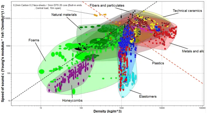
The acoustical performance of a material depends primarily on its density ρ and Young’s modulus E. Three important acous-tical properties are based on those two properties: the speed of sound c within the material, the characteristic impedance z and the sound radiation coefficient R. The values of these properties can be calculated using Equations 1. The value of the impedance is important for the transmission of vibrational energy from one medium to another. The incident intensity I0 is reflected to a

sound intensity Irand transmitted to the second medium at an

intensity Itaccording to Equations 2 with z1and z2 being the

impedance of the first and second medium, respectively. An ex-ample of such a transmission is the vibrational energy of the bowed string to the soundboard. If the difference in impedance of string and soundboard is excessively large, the transmitted energy is very small. This energy trends towards zero the larger the difference. The impedance of a soundboard is proportional to the characteristic impedance of the material but also to the square of the thickness of the plate [10].

c = s E ρ z = c · ρ = p E · ρ R = c ρ= s E ρ3 (1) I0 IR = (z2− z1 z2+ z1 )2 I0 IT = 4 · z2· z1 (z2+ z1)2 (2)

wood as a material has many different types that serve differ-ent purposes. Within one specific type there is variability as no two wooden pieces are ever exactly the same. This makes it im-possible to build instruments of consistent tone quality in com-bination with the nature of hand processes [11]. Wood reacting and adapting to its environment increases this variability even more. This variability, the endangered state of the frequently

used wood types and are the lower sensitivity to humidity [12]. The versatility and variety in composite materials is the reason why they are omnipresent across the entire world. Artists can create a product of any complex shape, translucency or colour that is very wear-resistant, while engineers can use it in all types of structures. There is no reason that violins cannot be made out of them except for relatively little research into their acoustics.

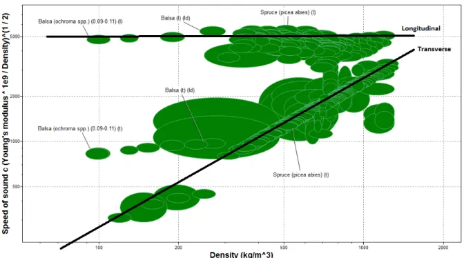
Similarly to different wood types, the acoustical performance parameters can be compared between different material groups in the material property plot shown in Figure 3. It can be noticed that wood is plotted twice on the same vertical line due to the significant different in Young’s modulus between the transverse and longitudinal direction. The two red lines represent constant sound radiation coefficient and speed of sound, respectively. It can be seen that the speed of sound is similar for the composites and wood along the grain. The same can be said about the spe-cific stiffness as it is the square of the speed of sound. The sound radiation coefficient is similar as well. However, the impedance of the composites is higher than that of wood types. All of this seems to indicate that composite material can definitely be used as material for the violin but that the acoustics should be evalu-ated using some type of setup.

IV. IMPACT MEASUREMENT SETUP

A setup to measure the radiation due to a certain impact exci-tation is made, shown in Figure 4 inspired by the one constructed by Curtin. The violin is vertically supported by two elastics un-derneath its tail end and its neck is supported horizontally be-tween two elastics. This is a compromise bebe-tween approximat-ing the free-free boundary conditions to limit the change in nat-ural characteristics and a stable system that holds the instrument in place to prevent full-body vibrations due to insufficient damp-ing and possible accidents. As the strdamp-ing energy is transmitted for the most part to the bridge, the modes of importance are the ones that can be driven from the bridge [14]. Therefore, the violin is excited at the bridge by an impact hammer suspended like a pendulum. The impact hammer should be small enough to impact the thin edge of the bridge properly. In the following discussions, a horizontal impact refers to an excitation near the top of the bass side of the bridge, while a vertical impact refers

to an excitation at the middle of the bridge top.

The suspension point of the hammer can be moved accurately in three orthogonal direction using a 3-axis assembly and it can be rotated to turn the striking tip when changing between differ-ent impact oridiffer-entations. The radiation resulting from the vibra-tions induced by the excitation is measured with a microphone positioned horizontally at the bridge from a certain distance. It should be quite flat to be sufficiently qualitative for good violin measurements. The height of the microphone and its distance to the violin can be adjusted as well. The impulse and response signal are transferred to the audio interface by the impulse ham-mer and the microphone. The interface then passes the data to the post-processing software called Oberlin Acoustics App or ObieApp. The settings of the test need to be defined by the user in the software to generate the correct FRF.

The base plate that holds the violin can be rotated around its centre with a pre-set angle per measurement. The radiation around the entire violin body can be mapped by doing measure-ment along an entire revolution. The rotation device is placed on a camera tripod as the setup is made to be portable. These setups can be brought along when several violin makers gather at con-ferences in order to give them the opportunity to measure the radiation of their creations. Much of the same measurements can be performed using a hand-held hammer, an ordinary mi-crophone stand, and a simple frame from which to suspend the instrument. However, hand strikes with a mini-force hammer on a violin are inherently unreliable as the position, direction and force levels vary widely. The advantages of a specialized rig are mainly speed and convenience [7].

Fig. 4. Impulse measurement setup in Ghent

V. MEASUREMENTS

A. Experimental violins

Mobility measurements have been performed using acousti-cal excaitation and SLDV acquisition on all experimental vi-olins and Conventional. These tests were performed by Tim Duerinck, supervisor of this dissertation. The resulting FRFs are shown for the experimental violins in Figure 5 between 300 and 620Hz to clearly illustrate the peaks of the A1, CBR, B−1 and B

+ 1

modes. The position of each mode was identified by recognition

of their mode shapes to determine the modal parameters. These mobility measurements are needed because the signature modes cannot be identified solely using radiation measurements, like the CBR mode. This could not have been done with radiation measurement as the mode radiates little sound. Identifying the A1, B−1 and B

+

1 modes in radiation FRFs is extremely difficult

if not impossible as there can be multiple significant peaks and their order in terms of frequency is unknown, except for that of the B−₁ and B+₁ modes.

Fig. 5. FRFs of the mobility acquired using SLDV on acoustically excited experimental violins, courtesy of Tim Duerinck

The FRFs of the radiation measurements of the violin made with sandwich material due to horizontal and vertical impact taken in Paris are shown in Figure 6, Although there are plots for the other experimental violins, only one is shown to compare the different type of measurement. In this plot the position of each signature mode is indicated by a circle in a specific colour: A0 and A1 in red, CBR in yellow, B−1 and B

+

1 in green. The

position of each mode is taken at the maximum of a peak in the FRF around the frequencies found in Section ?? except for the CBR mode. That mode can appear either as a small peak, dip or neither in the curve because the mode shape does not convert a significant amount of energy into sound like for the other modes. The bridge hill is observable around 2kHz on the FRF of hor-izontal impact measurements, while the same cannot be said for the vertical ones. Compared to the other experimental violin the bridge hill for violin made with sandwich material seems to be positioned around a slightly lower frequency. The observable difference between the FRFs of the horizontal and vertical im-pact measurements are no surprise considering that the vertical impact on the bridge and thus excites the rocking mode of the bridge less than a horizontal impact. The opposite is true for the bouncing mode of the bridge resulting in a flatter hill in the FRF between 5 and 7kHz.

There are up to three setups used to acquire measurement data of the violins referred to as Ghent, Paris and USA. The names refer to the location where the setup is constructed. Measure-ments have been taken on all three of them for the violin made with Sandwich material. The FRFs of the corresponding mea-surements can be compared in Figure 7. Noticeable on the plot is that the valley between the A0mode and the subsequent modes

is even more shallow than the one in FRFs of measurements in Paris. It can be also be seen that the A1mode does not show up

Fig. 6. FRFs of horizontal and vertical impact measurements of violin made with sandwich material taken in Paris from 200 to 780Hz, signature modes encircled: A0(left red) and A1(right red), CBR (yellow), B−1 (left green)

and B+₁ (right green)

Fig. 7. FRFs of horizontal impact measurement of violin made with sandwich material taken in Ghent, Paris and USA from 200 to 780Hz, signature modes encircled: A0(left red) and A1(right red), CBR (yellow), B−1 (left green)

and B+₁ (right green)

For the FRFs obtained in Paris and USA the intensity of the A1

mode is the lowest of any of the significant modes encircled but for the FRF obtained in Ghent it is larger than that of the A0

and CBR mode. This is one indication that something related to the setup in Ghent occurs at a frequency of around 430Hz that causes a spike in the FRF.

VI. COHERENCE

The coherence is a variable that indicates how coherent sev-eral different measurements are. It can be plotted in function of frequency ranging from 0 to 1, with 1 being perfectly coher-ent measuremcoher-ents at that frequency and 0 meaning the oppo-site. Examples of coherence plots of the same violin are shown in Figure 8 and 9 with each curve being the coherence of five different measurement with the microphone at a fixed position.

ence function, while those taken at position 2 do not. There are multiple significant valleys that go under a value of 0.8. Espe-cially for the B+1 mode the coherence is dramatically low, being

smaller than 0.5. Based on the bad coherence of position 2 new measurements were taken a week later. It can be seen on Figure 9 that these have a much better coherence across the frequency region for both positions.

Fig. 8. An example of a good and bad coherence function of horizontal impact measurement taken in Ghent of UD Flax at position 1 and 2

Fig. 9. An example of two good coherence functions of horizontal impact mea-surement taken in Ghent of UD Flax at position 1 and 2

Low coherence values indicate that the FRF value of that fre-quency is not representable of the correct value. This can be caused by remaining vibration of violin due to the last impact during next impact. This vibration can combine with the new one causing a different excitation of the bridge. This results in a distorted FRF for each measurement increasing the odds of a bad coherence function. This effect can be stronger around some frequencies than around others. If the frequency of the signature

modes is known, their corresponding coherence values are visi-ble on the plot. The function is encircled at the signature mode frequencies similarly to earlier. It is important that coherence is sufficiently high at the frequencies of the signature modes to be able to draw conclusions from the averaged FRF.

A. Acoustical centre low-frequency radiation

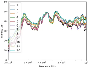
The measurement data used for this experiment was provided by Joseph Curtin. Eighteen measurements were taken on his setup in 2018 with wooden violins made by different luthiers as test instruments. A linear average was taken of the FRFs of all those measurements for twelve rotational positions of the test instrument separated by 30. At position 1 the violin top is facing the microphone, while at position 2 the violin is rotated coun-terclockwise from a perspective looking down at the violin. The averaged FRF for each position is plotted on Figure 10 for the horizontal impact measurements. Each averaged FRF follows a certain trend in terms of their proportion to each other up until a frequency of around 400Hz. A peak for one FRF is a peak for all the other, like the one at around 280Hz. It should be noted for each violin the A0 mode has a different frequency, but for

the purposes of this experiment that peak is seen as the result of the radiation of the A0mode since it is the first with a significant

intensity.

A polar plot of the intensity of the A0mode of averaged data

of multiple wooden violins is shown in Figure 11 for horizontal impact measurements. This A0 mode is found by locating the

point of maximum intensity around 280Hz. The frequency is the same for all twelve positions. It is clear that the A0mode

is louder in front of the violin than behind it. This indicates that the centre of radiation caused by the A0 mode is located

some distance in front of the centre of the violin. Based on the fact that the intensity increases with 6dB when the distance to the monopole source is halved, an approximate centre is found mathematically. This centre is illustrated by the green dot, while the red dots indicate which positions have the minimum and maximum intensity.

VII. CONCLUSION

Impact measurements on experimental violins result in FRFs similarly to those of wooden violins. Peaks can be found for several signature modes in the case of the experimental violins. However, there are some differences when comparing different violins. Solely replacing the wooden back and ribs by a one-piece composite already indicates that. The FRFs of the experi-mental violins are shifted to the lower end of the frequency spec-trum compared to that of the wooden violins. This is even more the case for violins with a soundboard made of unidirectional composite material. These violins have a significantly lower overall intensity than the other violins and a comparable shape of the FRF with the A1 and B+1 modes being the strongest

ra-diating modes. The A1, B−1 and B +

1 modes occur in this order

in terms of frequency for each experimental violin but not for the wooden violin. It is remarkable that the A0mode is the only

signature mode that is within a small frequency range for the experimental violins.

In a side experiment it was observed that this mode radiates as a monopole source from some distance in front of the centre

Fig. 10. FRF of the intensity of the A0mode for each of the twelve positions

using data acquired from linearly averaging of 18 sets of radiation measure-ments of different violins

Fig. 11. Polar plot of the intensity of the A0 mode for each of the twelve

positions using data acquired from linearly averaging of 18 sets of radiation measurements of different violins

of the violin body similarly to any sound wave of sufficiently low frequency. None of the violins with a soundboard entirely made out of carbon fibers and epoxy has a high peak for the B1+ mode thus having more emphasis on the lower frequency signature modes. Sandwich is the only violin made of carbon fibers that has a significant intensity for the B+₁ mode but this comes at the expense of some intensity of the A0 mode and the intensity peak nature of the A1 mode. Although this material

has a larger sound radiation coefficient, this did not result in a significant difference in the overall intensity. Remarkably it does have a similar FRF to that of Spruce.

Considering the low complexity of the construction, such a setup is quite useful and easy to use. Only five measurements at twelve positions are sufficient to get results that can be com-pared to other measurements. A test only requires about five minutes if everything goes correctly. However, care should be taken when setting the accept/reject parameters and changing

tively biased towards the use of novel materials that composite materials are very versatile and that violins made out of them belong in the violin family.

REFERENCES

[1] T. Duerinck et al., Experimental modal analysis of violins made from com-posites, 2018.

[2] P. Ball, Old violins reveal their secrets, 2008.

[3] C.M. Hutchins, A history of violin research. The Journal of the Acoustical Society of America, 1983.

[4] T. Duerinck, M. Kersemans, G. Verberkmoes, W. Van Paepegem and M. Leman, What’s the alternative?, The Strad, 2018.

[5] T. Duerinck et al., Listener evaluations of violins made from composites, The Journal of the Acoustical Society of America, 2020.

[6] J. Woodhouse, The acoustics of the violin: a review, Reports on Progress in Physics, 2014.

[7] J. Curtin, Measuring violin sound radiation using an impact hammer, J. Violin Soc. Am. VSA Papers, XXII, 2009.

[8] C. Gough, A violin shell model: Vibrational modes and acoustics, The Journal of the Acoustical Society of America, 2015.

[9] G. Bissinger, Normal mode analysis of violin octet scalings, Proceedings of the International Symposium on Musical Acoustics, 2001.

[10] U. Wegst, Wood for sound, American Journal of Botany , 2006. [11] J. Dominy and P. Killingback, The development of a carbon fibre violin,

17th International Conference on Composite Materials, 2009.

[12] A. Damodaran, L. Lessard, A. Babu, An overview of fibre-reinforced composites for musical instrument soundboards, Acoustics Australia , 2015. [13] H.R. Shercliff and M.F. Ashby, Elastic Structures in Design, Reference

Module in Materials Science and Materials Engineering, 2016.

[14] G. Bissinger, Modern vibration measurement techniques for bowed string instruments, Experimental Techniques , 2001.

Table of Contents

Permission for use of content i

Preamble ii Acknowledgements iv List of Figures xv List of Tables xx Abbreviations xxii 1 Introduction 1

2 Violins: Past, Present and Future 3

2.1 Parts . . . 3 2.2 Evolution . . . 7 2.3 Sound perception . . . 10 2.4 Sound Production . . . 11 2.5 Acoustics . . . 15 xi

2.6 Vibrational modes . . . 17 2.6.1 Bridge modes . . . 18 2.6.2 Plate modes . . . 19 2.6.3 Body modes . . . 20 2.7 Material . . . 21 2.7.1 Wood . . . 22 2.7.2 Composites . . . 25 2.7.3 Economical aspect . . . 33 2.7.4 Environmental aspect . . . 34 2.7.5 Vulnerability aspect . . . 34 2.7.6 Aesthetics . . . 35 2.8 Experimental instruments . . . 37

3 Methods for evaluating sound production 41 3.1 Modal analysis . . . 41 3.2 Excitation methods . . . 42 3.2.1 Impact testing . . . 43 3.2.2 Shaker testing . . . 44 3.2.3 Acoustical testing . . . 45 3.3 Measurement methods . . . 45 3.3.1 Mechanical measurements . . . 45 3.3.2 Optical measurements . . . 46

TABLE OF CONTENTS xiii

3.3.3 Indirect measurements . . . 46

3.4 Equipment or measuring devices . . . 46

3.4.1 Impact hammer . . . 46 3.4.2 Accelerometer . . . 47 3.4.3 Microphone . . . 48 3.4.4 Audio interface . . . 49 3.5 Setups . . . 49 3.5.1 Working principle . . . 50

3.5.2 Comparison different setups . . . 51

3.5.3 Aspects influencing measurement . . . 54

3.6 Oberlin Acoustics App . . . 64

3.7 Measurement quality . . . 67

3.7.1 Double bounce . . . 68

3.7.2 Coherence . . . 69

4 Measurements and discussion 73 4.1 Mobility measurements . . . 73

4.2 Radiation measurements . . . 76

4.2.1 Setup in Paris . . . 77

4.2.2 Setup in Ghent . . . 90

4.2.3 Setup in USA . . . 91

4.3.1 Different elastics . . . 96

4.3.2 Pliability of impact hammer handle . . . 98

4.3.3 Reproducibility setup . . . 99

4.3.4 Microphone distance to bridge . . . 100

5 Conclusion 102

Appendix i

Appendix A - ObieApp math ii

Appendix B - Construction Manual of Setup viii

Bibliography i

List of Figures

2.1 Exploded-view drawing of the violin with indicated parts . . . 4

2.2 Illustrating of the tuning of each strings by turning the corresponding pegs to a specific musical pitch . . . 7

2.3 Evolution of the violin shape [1] . . . 8

2.4 Evolution of the sound hole shape and the flow velocity through it, illus-trated using a normalized colour scale [2] . . . 9

2.5 Trapezoidal violin model of Savart and guitar-shaped violin model of Chanot [2] . . . 9

2.6 Simple example of Fast Fourier Transform of a waveform . . . 11

2.7 Contours of perceived equal loudness per frequency [3] . . . 12

2.8 Illustration of the complex feedback loop of sound production [3] . . . 13

2.9 Illustration of the stick-slip motion of the violin bow on the string [4] . . . 13

2.10 The transformation of the bowed string input waveform into the radiated sound by the bridge and body shell resonances for one selected note. Ver-tical dashed lines: Frequencies of the bowed string partials [5] . . . 14

2.11 Comparison total versus monopole radiation [6] . . . 16

2.12 Monopole, dipole and quadrupole source [3] . . . 16

2.13 First two vibrational modes of the violin bridge [6] . . . 19 xv

2.14 Chladni method with glitter and a speaker . . . 20 2.15 Mode shape of each signature mode of the guitar-shaped violin body [7] . . 21 2.16 Material property plots for different wood types [8] . . . 23 2.17 Theoretical speed of sound in function of density for different wood types,

courtesy of Tim Duerinck . . . 25 2.18 Young’s modulus plotted in function of density for different material groups

[9] . . . 26 2.19 Different weave patterns and their appearance using carbon fibre tows [10] 28 2.20 Regular tow vs. spread tow [10] . . . 29 2.21 Flaxtape made by Lineo [11] . . . 30 2.22 Longitudinal specific stiffness carbon, flax, and glass fibre reinforced plastic

[12] . . . 31 2.23 Schematic of a typical honeycomb core sandwich panel [13] . . . 32 2.24 Wooden violin with a graphite-epoxy soundboard substitute [14] . . . 32 2.25 Theoretical speed of sound plotted in function the density for different

material groups, courtesy of Tim Duerinck . . . 33 2.26 Several aesthetic carbon fibre patterns [10] . . . 36 2.27 Creativity expressed in string instruments [15] . . . 37 2.28 Experimental violins with different top plates. soundboard material from

left to right: (1) Twill woven carbon fibres, (2) Unidirectional carbon fi-bres, (3) Spruce, (4) Unidirectional flax composite, (5) Carbon-Nomex Sandwich, (6) Twill woven carbon fibres [16] . . . 38 3.1 Impact test setup [17] . . . 43 3.2 Shaker test setup [17] . . . 44

LIST OF FIGURES xvii

3.3 Two types of accelerometers used in excitation tests . . . 48

3.4 Phantom power schematic of a XLR cable [18] . . . 49

3.5 Three impact measurement setups . . . 52

3.6 Close up of mechanism holding the impact hammer . . . 53

3.7 Measuring equipment used in setup made in Ghent . . . 56

3.8 Required devices for construction of setup . . . 57

3.9 Example of sound spectrum in ObieApp . . . 65

3.10 Practical frequency bands of violins and their centroids plotted over FRF in ObieApp . . . 67

3.11 Three smoothing possibilities of ObieApp . . . 67

3.12 Two types of double bounces . . . 68

3.13 FRF for different mic cutoff values . . . 70

3.14 Hammer cutoff before double bounce (above) versus hammer cutoff after double bounce (below) . . . 71

3.15 Two examples taken on different days of coherence plots of horizontal im-pact measurements taken in Ghent on UD Flax at position 1 and 2 . . . . 72

4.1 FRFs of the mobility acquired using SLDV on acoustically excited experi-mental violins, courtesy of Tim Duerinck . . . 74

4.2 FRFs of the mobility acquired using SLDV on acoustically excited Con-ventional showing the frequency region for A0 and B0 courtesy of Tim Duerinck . . . 75

4.3 Table with signature modes of the experimental violins and their modal parameters courtesy of Tim Duerinck . . . 75

4.4 FRF of the mobility acquired using SLDV on acoustically excited Conven-tional courtesy of Tim Duerinck . . . 76

4.5 FRF of each violin for horizontal and vertical impact measurements in Paris from 200 to 7000Hz, signature modes encircled: A0 (left red) and A1 (right red), CBR (yellow), B−

1 (left green) and B +

1 (right green) . . . 79 4.6 FRF of each violin for horizontal and vertical impact measurements in

Paris from 200 to 780Hz, signature modes encircled: A0 (left red) and A1 (right red), CBR (yellow), B−

1 (left green) and B +

1 (right green) . . . 81 4.7 Comparison of the FRFs of Spruce and Conventional (wooden violin) in

the 200-700Hz range . . . 83 4.8 Comparison of the FRFs of horizontal impact tests taken in Paris on

TwillCA and TwillCB in the 200-700Hz range . . . 84 4.9 Comparison of the FRFs on horizontal impact tests on TwillCB on two

different dates: TwillCB (earliest) and TwillCBbis (latest) . . . 85 4.10 Comparison of the FRFs of horizontal impact tests taken in Paris on Spruce

and TwillCB in the 200-700Hz range . . . 86 4.11 Comparison of the FRFs of horizontal impact tests taken in Paris on

TwillCB and UD Carbon in the 200-700Hz range . . . 88 4.12 Comparison of the FRFs of horizontal impact tests taken in Paris on UD

Carbon and UD Flax in the 200-700Hz range . . . 89 4.13 Comparison of the FRFs of horizontal impact tests taken in Paris on

TwillCB and Sandwich in the 200-700Hz range . . . 90 4.14 FRFs of each violin for horizontal impact measurements in Ghent and Paris

from 200 to 700Hz, signature modes encircled: A0 (left red) and A1 (right red), CBR (yellow), B−

1 (left green) and B +

1 (right green) . . . 92 4.15 Comparison of the FRFs of horizontal impact tests taken with USA setup

on Sandwich and UD Carbon in the 200-700Hz range . . . 93 4.16 FRF of two experimental violins, horizontal impact measurement in Ghent,

LIST OF FIGURES xix 4.17 FRF and polar plot of the intensity of the A0 mode for each of the 12

positions using data acquired from linearly averaging of 18 sets of radiation measurements of different violins . . . 97 4.18 FRFs of horizontal impact measurements on TwillCB using setup in Ghent

with different elastics at the neck: two thin elastics (green), two thicker elastics (yellow) and one of each (blue) . . . 98 4.19 Thick elastics with reference lines for placing same violin models . . . 99 4.20 Difference in hammer spectrum based on impact hammer handle used on

TwillCB: a metal handle or a rubber handle . . . 99 4.21 FRFs of horizontal impacts measurements on TwillCB using the setup in

Ghent before (yellow) and after (green) disassembling and reassembling the setup . . . 100 4.22 UD Flax for mic distance at 10cm (red), 20cm (green), 30cm (yellow),

List of Tables

3.1 Measurement conditions of each setup . . . 55 3.2 Total weight of the violins (including strings and chinrest) and their

per-centage difference relative to TwillCB . . . 58 4.1 Frequencies of signature modes in Hz for acoustically excited Conventional

using SLDV acquisition courtesy of Tim Duerinck . . . 76 4.2 Intensity I and frequency f of signature modes for all experimental violins

and Conventional based on horizontal impact measurement in Paris . . . . 78 4.3 Intensity I and frequency f of signature modes for all experimental violins

and Conventional based on vertical impact measurement in Paris . . . 78 4.4 Averaged intensity I in dB and centre of mass C in Hz of different frequency

bands for each violin in horizontal impact measurements in Paris . . . 80 4.5 Averaged intensity I in dB and centre of mass C in Hz of different frequency

bands for each violin in vertical impact measurements in Paris . . . 82 4.6 Intensity of the signature modes in dB based on horizontal impact

measure-ments done on two separate dates normalized to TwillCB and the difference compared to TwillCB . . . 86 4.7 Signature mode frequencies of each experimental violins and the

conven-tional violin from measurements by the setup in Ghent . . . 87 xx

LIST OF TABLES xxi 4.8 Signature mode frequencies of each experimental violins from Ghent

mea-surements . . . 91 4.9 Difference in intensity of the signature modes relative to the intensity of

the A0 mode for measurements on Sandwich with different setups . . . 94 4.10 Intensity (dB) of each signature mode relative to that of the A0 mode for

measurements on UD Carbon with different setups . . . 95 4.11 Averaged intensity over 200-7000Hz of horizontal impact measurements on

UD Flax at different microphone distances with the setup in Ghent relative to that with a microphone at 30cm. . . 100

Abbreviations

CFRP = carbon fiber reinforced plastic

SLDV = scanning laser Doppler vibrometer FFRP = flax fiber reinforced plastic

FFT = Fast Fourier Transform FRF = frequency response function FRP = fiber reinforced plastic LDV = laser Doppler vibrometer

”A good impression can work wonders.” ~J.K. Rowling

1

Introduction

The violin is an age-old instrument that has gone through a long evolution that has defined western music ever since its creation. It evolved rapidly until around the 18th century when the Italian masters made violins of such quality that tests are still performed on them in the 21st century [19]. The sound of these violins is so good that researchers have been on a quest to find their secrets [20]. However, innovation never stops and there is a long history of small alterations to the old violins. The shape and material used for the larger parts of the violin did not change, although some tried to change the shape[21]. Different types of wood were the best material available for the acoustical properties of the violin parts. The creation of composites breathed new life in this part of the violin design. Violins partly made with this type of material were already made by luthiers in the second half of the 20thcentury [22]. At this time, it is not a novel idea to use composite materials as a violin, but wood is still by far the most frequently used material for those violin parts. Six experimental violins have been made in the same model with different types of composite materials. Their back and ribs are made of one entire part in carbon fibre reinforced plastic for all of these violins. The only difference is the material used for the soundboard ranging from spruce to an even more complex composite material made of outer carbon fibre reinforced plastic sheets and an aramid honeycomb core [23]. The

goal of these violins is not to imitate the sound of traditional violins, but rather illustrate that sound produced by violins made of composite materials can produce a pleasant sound. A panel of listeners has been subjected to violinists playing these instruments [24]. However, not every luthier has access to a well-chosen panel of listeners. Objective measurements provide a solution in that regard if the violin maker knows how to read the results. Fortunately, there has been much research into the acoustics of the traditional violin [4]. There exist different methods to investigate the acoustics of a self-made violin, but these are either subject to a high level of variability or are priced at a substantially high number. Joseph Curtin has made a relatively inexpensive and portable setup that uses an impact hammer to excite the violin with an acceptable variability [25]. This setup has served as inspiration in making a setup at Ghent, the location of this thesis to compare the experimental violins among themselves and to a traditional violin of the same model. The setup in combination with a computer software that is designed to transform the impulse signal measured by the impact hammer and the response signal measured by the microphone to a frequency response function. Although the excitation of the bridge does not produce the same sound as excitation of the strings with a bow, it allows a standardized approach to examining certain acoustical properties of the violin. In this master’s dissertation this method is used to compare the experimental violins and obtain an idea of the effect of replacing the material used in the violin by a composite material.

”Music is not math, it’s science. You keep mixing the stuff up until blows up on you, or it becomes this incredible potion.”

~Bruno Mars

2

Violins: Past, Present and Future

In this first chapter the most important violin parts are briefly explained first to provide the readers a introduction to common terms if they might be less familiar with the in-strument. Next the evolution of the violin is discussed, followed by a discussion about the sound perception. After this the sound production is discussed by explanation of the playing principle of the violin. The acoustics and vibrations of the violin are looked into as well. The material of the violin is next, both the traditional woods used and the newer fibre reinforced composites. The construction is different for these materials and the eco-nomical, environmental and vulnerability aspect are discussed as well as the aesthetics of the violin. The experimental violins used in this thesis are introduced and a summary is given of this chapter.

2.1 Parts

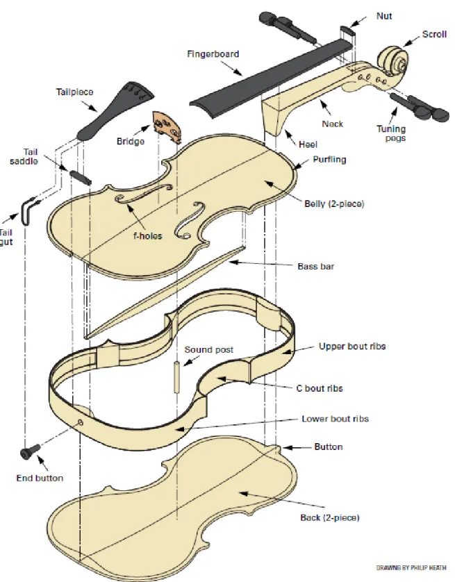
The violin is complex instrument with many parts that each have their position and function. An exploded-view drawing of the violin makes it clearer where each part is

2.1. PARTS 5 situated and how it is called. An example of such a view is shown in Figure 2.1.

The two largest parts of the violin are the top and back plates. The top plate is also called the soundboard, belly or face of the violin. These two plates are arched for strength and tone power. In most cases, each plate has a variable thickness decreasing from centre to edge. The top and back are usually made from spruce and maple, respectively, although poplar or willow are sometimes used in Baroque instruments [26]. The top and back are connected by the ribs and by the sound post. The ribs are made from six bent wooden pieces and six connecting blocks. The top, back and ribs form the body or soundbox of the violin.

The body is the biggest part of the violin and its aesthetic properties are critical to its appearance. Although the characteristic waist of the violin can be seen as aesthetically pleasing, it is in actuality a cut that allows violinists to bow each string without hitting the body. The largest part of an object is always the most likely to be accidentally damaged and that is where the purfling comes in. The ornamental border along the perimeter of both the top and back plate protects the top and back plate from cracks caused by accidental bumps. The f -shaped sound holes in the top plate, or f-holes for short, make it possible for air to freely enter and leave the body whenever its volume changes. This air flow and the vibrations of these large plates are big contributors to the sound production of the violin making them two of the most important violin parts.

The bass bar is a long, slender strip of wood that is glued under the top plate in the direction of the strings. In Figure 2.1 it is drawn at the wrong location as it should be underneath the bass feet of the bridge, or left side in from that perspective. Its function is reinforcing the strength of the top and for that reason its bottom is curved along its length. The bass bar enriches the tone of the lower notes. Contrary to its name, the bass bar has more effect on the treble than the bass of the violin.

The ribs may be the part with the most obvious function being that is holds the top and back plate together. However, there is a small, unvarnished wooden cylinder that connects the two as well and is called the sound post. In the earliest reported studies of the violin in 1840 Felix Savart remarked the following: ”This mobile piece plays the most noteworthy part in the violin, for without this piece its sound is very weak and of poor quality.” [27] The crucial function of the sound post is transmitting vibrations between the two plates, thus enhancing the volume and tone of the violin. It is positioned between the symmetry axis of the top plate and the right f-hole, kept in place purely by friction and can be seen through that f-hole upon a closer look.

The bridge is another small, unvarnished part that has a crucial function in the violin. This complex shaped part is kept in place by friction with the violin top and the downwards pressure of the strings that run through incisions at the top of the bridge. The exact position of the bridge is in the middle of the little crossbars of the f-holes, perpendicular to the symmetry axis of the violin. At this location it transmits and amplifies the string vibrations to the violin body. This function is discussed more in detail in Section 2.6.1. The fingerboard, bridge and tailpiece are all slightly curved in a similar way in the trans-verse direction to enable the player to bow each string separately. While the fingerboard is glued to the neck of the violin, the tailpiece is fixed through the tail gut by the end button. Neither touches the violin top as this would disrupt its sound production. When the fingerboard makes contact with the violin top, it produces a rattling sound because of the violin top vibration and could even cause damage to the top. All of this is prevented by letting the tail gut pass over a ridge that is called the saddle and the applying enough tension on the strings at the other end of the tailpiece. Minor tuning adjustments are possible on that end via small metal screws fitted on the tailpiece.

The strings are made of gut or synthetic material and run from the tailpiece over the bridge to the peg box. When a violinist plays very dramatically, the strings are bowed with great force. The height of the bridge prevents the strings from clattering on the fingerboard. The lowest tuned string is the one that allows the most strain. The bridge is slightly asymmetrical on the side of this string to prevent the disruption of the produced sound.

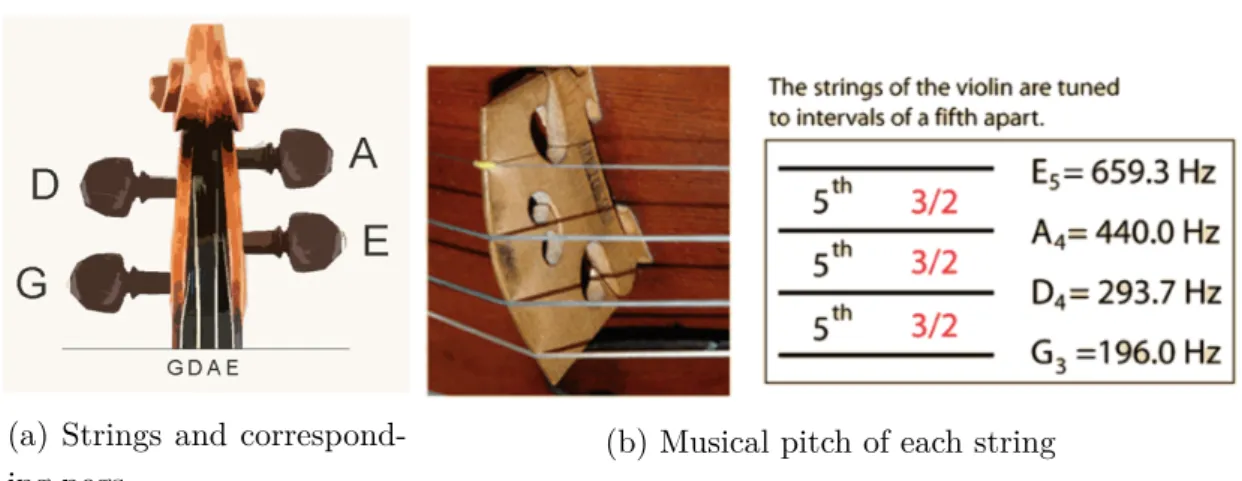
The peg box is a rectangular box that is connected to the violin body by the neck. It has four holes, one for each turning pegs. The violinist can tune each string by turning one peg. This tightens or loosens the strings depending on the rotation direction. Music instruments are always tuned to an A-note and violins are no exception. When looking straight at the soundboard, the third string from the left is tuned to the musical pitch A4 corresponding to a frequency of 440Hz as can be seen on Figure 2.2a. This figure also shows which peg should be tuned for to influence each string. The four strings are tuned in perfect fifths, meaning that the frequency of each string should increase in frequency with a factor 27/12, or approximately 1.5, from left to right. The musical pitch corresponding to each frequency is G3,D4,A4 and E5, in increasing order. Figure 2.2b shows the values of these frequencies and shows how the strings keep the bridge in place. A raised ridge at the base of the peg box, called the nut, stops the string from vibrating. Finally, a scroll is made on the other end of the peg box, derived from the paper scroll that was used as communication during the early days of the violin.

2.2. EVOLUTION 7

(a) Strings and

correspond-ing pegs (b) Musical pitch of each string

Figure 2.2: Illustrating of the tuning of each strings by turning the corresponding pegs to a specific musical pitch

2.2 Evolution

This summary of the evolution of the violin was written using information out of Chapter 2 of the book ’Handbook of materials for string musical instruments’ written by Bucur. String instruments played by a bow migrated from the Far East to Europe. Two in-strument families are seen as ancestors to the violin family: the rebec and the vielle. They travelled a different path with different tribes. Instruments from the rebec family are characterised by a pear-shape, significant arching at the bottom, having three strings that are tuned in fifths and no nut at the base of the peg box. In comparison, instruments from the vielle family resemble the current violin more, although they have a longer and deeper body. In contrast to the modern violin, they had a variable number of strings, three to five, and frontal tuning pegs.

At the end of 15th century lira da braccio, which meant held in the arms, appeared in Italy. This earliest version of this instrument had seven strings. Five on the fingerboard, tuned in fifths, meaning that the tuning frequencies of strings increased by a factor 1.5, similarly to the modern violin. The two other strings were not located on the fingerboard and tuned in octaves.

The violin family emerged in the 16th century as a consequence of the evolution of rebec and lira da braccio. The construction of the viola was a derivation of these two instrument families. The violin and violin cello were constructed similar to the viola but designed to have a higher and lower pitch, respectively. The violin family was originally composed

(a) Ancestors (b) Violin family

Figure 2.3: Evolution of the violin shape [1]

of these three but later accompanied by the double bass when it appeared from another family, the viol family, in a modified version.

The instruments manufactured in Cremona or Brescia, Italy, during the 16th and the 17th century are considered by many luthiers today as the peak of their craft. The acoustical advancements of the family are owed to the great Cremonese masters like Antonio Stradivari. The design of his violins was accepted as the definitive reference by later generations of violin makers according to Bucur.

The advent of Baroque music and later Romanticism came with new technical require-ments for the violin family to provide a different sound. However, the shape of the violin was unaffected by the passing of new styles. The graceful outline, harmonious propor-tions, and the minimal use of ornamentation explains in part why the violin has resisted significant stylistic modification to this day. Ever since, violin maker masters have tried continuously to reproduce these models and their supreme acoustics.

The steady evolution of the body from the rebec and vielle to the modern violin family is illustrated on Figure 2.3. The body of each member of the violin family is very similar when scaled to same length. There are other parts that have gone through their own evolution such as the sound hole and the bridge.

The sound hole geometry of the violin’s ancestors slowly evolved over centuries from simple circles to complex f-holes, as can be seen in Figure 2.4. This innovation was the

2.2. EVOLUTION 9

Figure 2.4: Evolution of the sound hole shape and the flow velocity through it, illustrated using a normalized colour scale [2]

Figure 2.5: Trapezoidal violin model of Savart and guitar-shaped violin model of Chanot [2]

result of maximizing the efficiency of the flow near the outer perimeter. This efficiency roughly doubled the air resonance power efficiency. The length of the f-hole then slowly increased by roughly 30% across two centuries [2].

For every evolution there are unsuccessful evolutionary offshoots that do not catch on. Two violin models that have one or more significant differences with the modern violin are shown in Figure 2.5. Savart and Chanot used their scientific background to steer away from the traditional shape of the violin parts based on preconceptions.

The trapezoidal model of Savart is the closest to a symmetrical violin found in the research done for this dissertation. This symmetrical approach was due to his belief that the more balanced the instrument is, the easier and more symmetrical the body can vibrate resulting in a more beautiful sound [28]. Therefore, the bass bar is positioned along the symmetry axis instead of under the bass foot. The sound post is the only asymmetrical element of the violin as it cannot be placed at the centre of the sound holes.

2.3 Sound perception

The sound produced by violins is designed to be pleasantly perceived by humans so the human range of hearing needs to be considered. A young adult can usually hear musical sounds from around 20 Hz to 16 kHz, with the high-frequency response decreasing somewhat with age. This large dynamic range of sound levels that humans can perceive is exploited by an orchestra. It needs many different instruments and most produce sound that covers a large frequency region. One instrument usually has a range of about 45dB [3]. Violins are prominently present in orchestras. As all violins produce such a unique sound, they are classified using descriptors such as bright, loud and warm. The sound from a violin observed by the player is even different than the sound that the audience hears. This is discussed more in detail in Section 2.5. The important frequency range for this perception is 190 to 7000Hz as 190 Hz corresponds approximately to the violin’s lowest note [29].

The frequency spectrum of music and its intensity are both perceived in a logarithmic scale. In the musical spectrum there are seven octaves. One octave covers a range of frequencies with an upper frequency twice the lower frequency. An octave can be divided into six tones or twelve semitones. The frequency of each semitone is larger than the previous one with a factor 21/12 or 1.059. Humans observe sound in pitch, even if the pitch is not a fundamental frequency, such as when two bowed strings are played a fifth apart similarly to the example in Figure 2.6. The waveform clearly has a pitch of 100Hz in the time domain, while there is no peak visible in the frequency domain. The waveform is in actuality a superposition of two sinusoidal waves of 200Hz and 300Hz that are being played simultaneously, causing humans to perceive a pitch of 100Hz.

Sound pressure levels (SPL) and intensity level (IL) are measured in dB relative to a reference pressure level p0 and I0, respectively.

SP L = 20log10( p1 p0 )with p0 = 2 ∗ 10−5 (2.1) IL = 10log10( I1 I0 ) with I0 = 10−12W/m2 (2.2)

A large range of sound intensity can be perceived by humans without experiencing pain. The upper limit is 120dB as the ear experiences pain and potential permanent damage

2.4. SOUND PRODUCTION 11

(a) Original waveform in time domain

(b) Original waveform in fre-quency domain

(c) Split waveforms in time do-main

Figure 2.6: Simple example of Fast Fourier Transform of a waveform

[3]. The higher the sound intensity above this value the more pain and damage. Sound at 150dB causes rupture of the eardrum. However, damage is possible even at lower sound levels such eight hour exposure to sound at 80dB. Some other example for sound levels are given here as references. A calm conversation at home is perceived at 50dB, while silence in that home in a suburban area clocks in at 30dB. A quiet recording studio has a sound level of 20dB while breathing is perceived at 10dB. Finally, acoustic measurements are best taken in anechoic rooms since these are designed to have a sound level of 0dB. Interestingly enough, humans are more sensitive to an increase of intensity at lower frequencies. In Figure 2.7 contours are plotted through sound level at each frequency that is perceived of be of equal loudness by a test audience. At lower frequencies the curves lie closer together meaning that the average human senses an increase in sound level more when the frequency of the sound wave is low.

2.4 Sound Production

The production of sound of any violin is based on the same acoustic principles. The player excites the vibrations of a string by bowing it. Energy from the vibrating string is then transferred via the supporting bridge to the acoustically radiating parts of the instrument. Experienced violinists have trained years to intuitively feel with how much force and at what angle each string needs to be bowed to produce a certain sound. Playing the instrument has become second nature to them and their playing style is different from another player. A number of stages occur between the violinist bowing the string and

Figure 2.7: Contours of perceived equal loudness per frequency [3]

the sound being perceived by a listener. This is illustrated in the complex feedback loop shown in Figure 2.8.

The complexity of this loop can be decreased by splitting it into multiple processes. The string is bowed until it experiences a certain strain where it slips back in the opposite direction. The antinode of the string moves towards one of the fixed ends at one side of its equilibrium line and back towards the bow on the other end. The bow still moving in its original direction picks up the antinode and drags it along until the process is repeated. This stick-slip motion is illustrated on Figure 2.9, while the simplified displacement of the point on the string during that motion is shown in Figure 2.10.

The vibrating strings holding the bridge feet onto the sound plate excite the bridge through its incisions at the top. The bridge vibrates and passes its vibration onto the soundboard through its feet. The soundboard is connected to the rest of the body and resulting in vibration of the entire body. Since the body is not a closed volume but in contact with the surrounding air through its sound holes, the volume in the body is constantly changing. The vibration of the air and the violin plates produce the observed sound.

The production of the sound by a violin can hence be simplified to this: the string is bowed, the string claps back, the bridge vibrates and the body vibrates. The input waveform of the string that is bowed and slips can be Fast Fourier Transformed (FFT) since every waveform is a superposition of many sinusoidal waves with a certain period

2.4. SOUND PRODUCTION 13

Figure 2.8: Illustration of the complex feedback loop of sound production [3]

Figure 2.9: Illustration of the stick-slip motion of the violin bow on the string [4]

and amplitude. A simple example of FFT is shown in Figure 2.6b. In the top figure of Figure 2.10 the peaks occur at multiples of the natural frequency, being the frequency of the first peak.

Figure 2.10: The transformation of the bowed string input waveform into the radiated sound by the bridge and body shell resonances for one selected note. Vertical dashed lines: Frequencies of the bowed string partials [5]

The body shell response shown in Figure 2.10 is the frequency response function (FRP) of the violin body without the bridge. The measurements done with the setup discussed in Section 3.5 present the body shell response passed through the bridge filter. This total response function serves as a filter for the FFT of the input waveform resulting in the FFT of the output waveform. This can then be transformed back to a function in the time domain.

For each string the input waveform is different and bowing the string at different points of a string results in different strain at which it slips from the bow. The relation between bowing the string and producing the sound is complex since the body vibration caused by the bowing affects the absolute movement of the string. For that reason, it is difficult

2.5. ACOUSTICS 15 to reproduce the process of playing a violin with an excitation test.

2.5 Acoustics

This summary of acoustics was written using mostly information out chapter 15 of the book ’Handbook of Acoustics’ written by Rossing.

A near and far field can be defined based on their value of kr, with k being the propagation speed and r being the distance to the source. For the near field, this value is smaller than one, while the opposite is true for the far field. The importance of this distinction lies in the phase difference of the pressure and velocity of the sound wave. Pressure and velocity differ in phase by an amount that depends on the distance from the source and the wavelength. In the near field the pressure and velocity are in phase quadrature. This means that no work is being done on surrounding air since it is proportional to R pvdt, while the opposite is true in the far field where the pressure and velocity are in phase. The transition area of these two fields has a value of around one for kr. Knowing that k = ω/c, λ = c/f and ω = 2πf, this boundary is achieved when r = λ/2π with λ being the acoustic wavelength. As the value of that wavelength depends on the speed of sound and the frequency the transition area is different for every frequency. The higher the frequency the smaller the near field and the more likely the ear of the violinist is outside this field. For low frequencies this distance is large causing the violinist to be in the near field. This means that the violinist observes a different sound than the audience sitting at a larger distance from the source.

The upper line shown in Figure 2.11 is the estimated total radiation while the lower line is the monopole radiation in function of the frequency. The lines are almost coincident for frequencies lower than 1kHz. This means that the instrument radiates more-or-less as a monopole at low frequencies [6]. For higher frequencies this is no longer the case as λ has become comparably small as the physical size of the instrument. The musical source can then be seen as a superposition of monopole, dipole, quadrupole and higher-order multipole acoustic sources. A dipole source can be formed by displacing two equal but oppositely signed monopoles a short distance along a certain direction. Doing the same with two dipoles results in a quadrupole source. These three types of sources are shown in Figure 2.12.

Figure 2.11: Comparison total versus monopole radiation [6]

2.6. VIBRATIONAL MODES 17 The transition from monopole source to superposition of different multipoles is caused by the sound acquiring directional properties determined by the geometry of the instru-ment and the vibrational characteristics of the excited modes. Six quadrupole sources are needed to describe radiation of a three-dimensional string instrument but increasing the order of a multipole source increases the intensity by two powers of the frequency. Therefore, the radiation is dominated by one monopole source for very low frequencies and by three extra dipole sources for low frequencies.

A large part of sound made by string instruments propagates from the vibration of the top and back plates. These instruments efficiently radiate the sound when the phase velocity of the transverse vibrations on the plate is higher than the speed of sound. This velocity increases proportional to the square root of frequency. There exists a critical frequency below which the plates radiate sound ineffectively and above which they do it effectively. Estimates by Cremer [30] of this frequency for a 2.5 mm violin plate and a 4 mm-thick cello plate are 2kHz and 2.8kHz, respectively.

The vibrating string is a linear dipole radiation source [31]. Dipoles are weak radiators at low frequencies meaning that strings are not a large radiation contributor since they are tuned to low frequencies. At those low frequencies most of the acoustic input is caused by the Helmholtz resonance of the air inside the instrument. This air vibrates in and out through the f-holes of the top plate. Since the strings do not radiate much sound, their energy is best passed on to the better radiating parts of the instrument, such as the top and back plate via the bridge. The plates are larger surfaces that can radiate more sound, all be it at higher frequencies.

2.6 Vibrational modes

All vibrations are a combination of both forced and resonant vibrations. Forced vibration can occur due to internally generated forces, unbalances, external forces and ambient excitation. Resonant vibration occurs when one or more normal modes of vibration of a structure is excited [17]. Modes are inherent properties of a structure. These are the material properties, such as mass, stiffness and damping properties, and the boundary conditions of the structure. Each mode is defined by a natural or resonance frequency, modal damping and the mode shape. If any of these properties change, the modes change along with it [3]. The mode shape is characterized by nodal lines, along which vibrational motion is at a minimum, and antinodes, where motion is at a maximum. A normal mode

can be excited by applying a force to any point on the structure that is not on a nodal line, excitation being strongest at resonance frequency.

2.6.1 Bridge modes

The bridge is a complex component of the violin that can be split into an upper and bottom part separated by a small waist acting as a spring. Figure 2.13 shows two important in-plane modes. The first bridge resonance occurs at a frequency of about 3kHz. Around this frequency the upper part rocks side to side and it is therefore referred to as the rocking mode. The treble foot of the bridge acts as a pivot for the vibration while the bass foot swings. The bass bar couples the energy to a large part of the soundboard by applying a couple via the bridge feet. The second mode occurs at about 6kHz. It is called the bouncing mode because the upper and bottom part bounce up and down at this frequency [3].

When the violin is played the bow exerts a lateral force on the strings at the top of the bridge. This is translated to a vertical force via its feet. Figure 2.10 already showed that the bridge behaves as a filter. Each resonance frequency functions as the resonance of a low-pass filter. The bridge behaves as a rigid body at frequencies well below the first resonance frequency. This allows the strings to act directly on the body. At resonance frequency, the bridge strongly reinforces the transmission of string vibration to the body. The string vibration is increasingly reflected from the bridge back into the string the higher the frequency than the resonance frequency. A local minimum is reached before the transmission increases in terms of frequency until the second resonance frequency is reached. Beyond that frequency the bridge reflects the string vibration again at an increasing rate [6].

Controlling the frequency of these two modes is called bridge tuning and is important for the sound production process of the violin. As the bridge is so complex, small and thin the smallest alterations can lead to large changes in the sound of the violin. These alterations can go from choice of material to shape details such as the thickness, height or overall proportions. Increasing the in-plane stiffness without modifying the bridge mass too much can be done by placing tiny wedges in the cutouts. While adding bits of modelling clay to the top of the bridge does not change the stiffness. Removing wood is also used to shift the mode frequencies [32].

2.6. VIBRATIONAL MODES 19

Figure 2.13: First two vibrational modes of the violin bridge [6]

2.6.2 Plate modes

Up until this point, the importance of the top and back plate has been stressed. They are undoubtedly the important violin components when determining the quality of the sound produced. Before constructing the body, a luthier can examine the vibration of both plates. One of the simplest methods is the Chladni method. The principle of this method is that particles can be acoustically levitated by the force of plate vibrations caused by sound at a fixed frequency. In 1787 Chladni reported the first detailed studies on the aggregation of sand onto nodal lines of a vibrating plate [33]. In his experiments he strewed sand onto circular, quadratic and rectangular plates to illustrate the patterns that formed on the plate [34]. However, when he used fine shavings of the hair of his violin bow, these did not follow the sand to the nodal lines but collected at the antinodes. The conditions under which a given material behaves as a nodal or antinodal line are discussed in detail by Waller. The particle diameter of sand should exceed 100 µm for it to form the nodal lines on a Chladni pattern [35]. Table salt can be used as an alternative to sand and flakes of glitter can be used on wood [36].

The use of these Chladni patterns remains an easy and inexpensive method to evaluate plate acoustics. Nowadays, a loudspeakers capable of inducing sufficient plate motion are placed underneath the plate to excite it with a sinusoidal wave. This meant that the plates did not have to be clamped for mechanical excitation but could float over the speaker on small foam supports and be acoustically driven, giving a much better approximation to the ideal free-free boundary [37]. Luthiers use these methods to fine-tune the top and bottom plate of their creations. When the frequency matches a plate mode, the plate vibrates vigorously causing the small particles to migrate towards the nodal lines as shown on Figure 2.14.

Figure 2.14: Chladni method with glitter and a speaker

This technique works well for the top and back plates which have concave surfaces. Un-fortunately, these surfaces are positioned on the inside in the assembled instrument. The outer surfaces are mostly convex surfaces resulting in powder rolling or sliding off them when the instrument is vibrated diminishing the utility of this method. However, some question this method and its correlation to the resulting frequency spectrum of the violin, such as Schleske [38].

2.6.3 Body modes

The frequency region relevant for this subject is chosen as 200Hz to 7000Hz. This region can be split into three parts: lower frequency region 200Hz to 1kHz, middle frequency region 1kHz to 2-3kHz and the higher frequency region. The collection of peaks in the 2–3 kHz is called the bridge hill. The modes of the lower frequency region are called the signature modes. They are referred to as the A0, A1, CBR, B−

1 and B +

1 modes in this thesis. Other names for these modes in literature are A0, A1, C1, C2 and C3, respectively [6]. Figure 2.15 shows the mode shape in terms of displacement of each of these signature modes for a guitar-shaped violin body. The A0, A1, CBR, B−

1 and B +

1 modes are referred to as c0, p2, p1, c2 and c3 modes in this figure. It should be noted that the colour scale is relative to the maximum displacement of each figure.

The A0 mode involves the top and back plate moving in opposite directions along the depth direction of the violin. It is associated with a strong sound radiation coming from the f-holes and is therefore referred to as the breathing mode. It is one of, if not the, most important modes in terms of acoustics [7]. A1 is the mode where air moves from the upper bout to the lower bout of the violin body. A1 can be a significant radiator of