Analyses van opties voor het opnemen van internationale luchtvaart en scheepvaart emissies in een post-2012 klimaat mitigatie regime

(1)

Netherlands Environmental Assessment Agency (MNP), P.O. Box 303, 3720 AH Bilthoven, the Netherlands; Tel: +31-30-274 274 5; Fax: +31-30-274 4479; www.mnp.nl/en

MNP Report 500114007/2007

An analysis of options for including

international aviation and marine emissions in

a post-2012 climate mitigation regime

M.G.J. den Elzen, J.G.J. Olivier, M.M. Berk

Contact:

Michel den Elzen

Global Sustainability and Climate (KMD) Michel.den.Elzen@mnp.nl

This research was performed as part of the study ‘Aviation and maritime transport in a post-2012 climate policy regime’ directed by CE Delft, which was conducted within the framework of the Netherlands Scientific Assessment and Policy Analysis (WAB) Climate Change Programme

(2)

Parts of this publication may be reproduced, on condition of acknowledgement: 'Netherlands Environmental Assessment Agency, the title of the publication and year of publication.'

(3)

Acknowledgements

This study was performed as part of a study led by CE Delft, entitled ‘Aviation and maritime transport in a post-2012 climate policy regime’, conducted within the framework of the Netherlands Scientific Assessment and Policy Analysis (WAB) Climate Change Programme. We would like to thank Jasper Faber (CE Delft) and David Lee (Manchester Metropolitan University) for their comments and contributions. Special thanks are due to the advisory committee, consisting of members of the different ministries, who have provided us with critical and useful comments.

(4)

(5)

Rapport in het kort

Analyse van opties voor het opnemen van internationale luchtvaart- en scheepvaartemissies in een post-2012 klimaatmitigatieregime

Een belangrijke conclusie van de analyse zoals gepresenteerd hier is dat het meenemen van bunkeremissies in nationale/regionale reductiedoelstellingen meer kosteneffectief is dan het niet meenemen en het voeren van apart sectorspecifiek beleid. De huidige snelgroeiende internationale lucht- en scheepvaartemissies zijn niet opgenomen in de nationale

reductiedoelstellingen onder het Kyoto Protocol. Een analyse is gemaakt van opties om internationale lucht- en scheepvaartemissies in toekomstig klimaatbeleid op te nemen. Er is specifiek gekeken naar twee nationale/regionale allocatieopties die vanuit klimaatbeleid het meest efficiënt lijken: allocatie volgens de nationaliteit/registratie en allocatie volgens bestemming. De consequenties voor de regionale reductiedoelstellingen van deze

allocatieopties voor deze zogenaamde bunkeremissies onder een post-Kyoto klimaatbeleid zijn geëvalueerd. Dit rapport presenteert een basisscenario voor de toekomstige

bunkeremissies tot 2050 en een CO2-reductiescenario voor deze specifieke sector gebaseerd

op een verhoogde verbetering van de energie-efficiency en het gebruik van biobrandstoffen. De nationale/regionale allocaties onder verschillende allocatieopties worden geanalyseerd en de implicaties voor reductiedoelstellingen in de andere sectoren zijn verkend. Ook het beperkte potentieel voor de reductie van de bunkeremissies zelf is geëvalueerd.

Trefwoorden: scheepvaart, luchtvaart, emissies, CO2, internationale bunkers, klimaatbeleid,

(6)

(7)

Summary

Analysis of options for including international aviation and marine emissions in a post-2012 climate mitigation regime

International aviation and shipping is projected to contribute significantly to international greenhouse gas emissions. These so-called bunker emissions are however not (yet) regulated by international policies under neither the UNFCCC nor its Kyoto Protocol. The aim of this study was to explore key options for dealing with including international bunker emissions in future climate policies, and to analyse their implications for regional emission allocations and global mitigation efforts.

The present analysis focuses on two options that seem most practical from a policy perspective: (1) allocation according to nationality/registration (SBSTA option 4) and (2) allocation according to destination (SBSTA option 6). The first option was selected as is fits in with the present regulatory regimes for international aviation and shipping in the context of the International Civil Aviation Organisation (ICAO) and International Maritime

Organisation (IMO). The second, route-related option was selected because of the availability of data on imports of goods by shipping.

In exploring the implications of allocating bunker emissions under a post-2012 regime for future commitments the Multi-Stage approach has been chosen here. This is an incremental but rule-based approach for defining future emission abatement commitments, where the number of parties taking on mitigation commitments and in their level of commitment gradually increases over time. These increases over time are according to participation and differentiation rules which are related to the countries level of development and contribution to the problem.

The baseline scenario used is the updated IMAGE/TIMER implementation of the IPCC-SRES B2 scenario. The B2 scenario is based on medium assumptions for population growth, economic growth and more general trends such as globalisation and technology development. This report presents a baseline scenario for future international bunker emissions up to 2050 and regional responsibilities under various regional allocation options. Next, various

scenarios for dealing with the international bunker emissions in future international climate policy are analysed. The report looks both at options of regulating bunker emissions as part of the Multi-stage regime and separately on the basis of sector policies, and also explore the implications for mitigation targets for the other sectors when international bunkers emissions are being abated or left unabated. Here we also evaluate the consequences of including the relatively high impact of non-CO2 emissions from aviation on radiative forcing in CO2

-equivalent emissions from international bunkers. The main findings of this study are:

• Due to the high growth rates of international transport in the B2 baseline scenario by 2050 the share of unabated emissions from international aviation and shipping in total greenhouse gas emissions may increase significantly from 0.8% to 2.1% for

(10)

international aviation (excluding non-CO2 impacts on global warming) and from 1.0%

to 1.5% for international shipping. These shares may seem still rather modest, however, compared to total global allowable emissions in 2050 in a 450 ppm

stabilisation scenario unabated emissions from international aviation have a 6% share (for CO2 only) and unabated international shipping emissions have a 5% share. Thus,

total unregulated bunker emissions account for about 11% of the total global allowable emissions of a 450 ppm scenario.

• However, since the total impact of aviation on radiative forcing is about 2.6 that of CO2 only (Radiative Forcing Index, RFI), by 2050 the share of international aviation

(including the RFI) in total greenhouse gas emissions in the baseline scenario will be about 5% instead of 2% for CO2 only. For the 450 ppm stabilisation scenario by 2050,

compared to total global allowable emissions the share of international aviation emissions increases from 6% to a 17%, and the share of international bunker emissions increases from 11% to about 20%.

• Incorporation of the non-CO2 impacts of aviation on climate change (e.g. as

represented by the Radiative Forcing Index) into the UNFCCC accounting scheme for greenhouse gas emissions should be considered, since aviation is a special case in this respect where the non-CO2 impacts constitute a significant contribution. Moreover,

aviation is expected to be one of the fastest growing sources and focussing solely on reducing CO2 emissions from aviation would likely be counterproductive from a

climate perspective: when improving the engine efficiency without further consideration and thus neglecting other climate pacts, e.g. NOx emissions will

increase and therefore the non-CO2 impact of aviation on climate change.

• Given the limited (cost-effective) potential for greenhouse gas emission reductions in this sector (without substitution to biofuel), the inclusion of bunker emissions in an international emissions trading scheme seems to be a more effective and cost-effective way of having the aviation and maritime sectors share in overall emission reduction efforts as opposed to the development of sector-based policies. Inclusion in an international emissions trading scheme would provide the international transport sector the opportunity to compensate their emissions by purchasing emission

reductions from other sectors instead of having to reduce their own emissions that are either very limited or very expensive.

More detailed findings on specific issues are:

Baseline developments

• Global international bunker emissions are projected to grow strongly in the period 2000–2050 (275% increase). The aviation sector is responsible for most of this growth.

• In 2050 the shares of the international aviation in total CO2 bunker emissions

increases from 45% to 60%. Including non-CO2 contributions to radiative forcing the

(11)

Allocation options

• Although the allocation of marine emissions to the flag states (Option 4) is not very robust, in practice the interchanges of registration to flag states over time have been limited during the past decades. At the present time, the registration of most ships is concentrated in the Bahamas, Panama, Liberia and Singapore as well as Greece, Malta and USA. However, for some ship types also China, Hong Kong, Norway, Germany and the Netherlands are among the most favourable flag states.

Consequently, for those countries, an allocation to flag states can have a large effect on their total national GHG emissions.

Environmental penalty

• If international bunker emissions were to remain unregulated and uncompensated, this would result either in higher emission reduction targets for specific Annex I regions in order to still meet the global emissions pathway stabilising at 450 ppm, or in a

significant surpassing of this emissions pathway – by about 3% by 2020 and 10% by 2050. These figures would double when the Radiative Forcing Index of aviation is included, implying that the stabilisation of greenhouse gas concentrations at 450 ppm CO2-eq. by 2100 would become difficult.

Mitigation penalty

• If international bunker emissions are excluded in a Multi-Stage regime approach, and these unregulated international bunker emissions are compensated by more stringent reductions in the other sectors regulated in the international climate regime, this would result in higher emission reduction targets for particular Annex I regions in order to still meet the global emissions pathway stabilising at 450 ppm. Including the RF impact of non-CO2 emissions from aviation would further increase the reduction

targets. For example, for the EU, the reductions compared to 1990 levels can become more than 20% in 2020 (instead of 12%) and 90% in 2050 (in stead of 75%).

Regional emission commitments

• If international bunker emissions are included in a Multi-Stage regime approach, the impacts of different allocation rules are relatively small at the regional scale.

However, this is not true for Central America, of which the amounts allocated have been shown to be very sensitive to the allocation rules used as the impact on

allowable emissions is relatively small.

• If the bunker emissions are included in the regime, but remain unregulated, and other sectors included in the regime compensate the bunker emissions (via emissions trading), this leads to high reductions for the Annex I regions. The reductions are comparable with those under the mitigation penalty case, although even higher for the US, EU and Japan due to their high aviation emissions. Including the radiative forcing impact of non-CO2 emissions from aviation would even imply zero-emission

allowances for those regions.

Sector-based emission reduction policy

• The effectiveness of sector-based emission reduction policy scenarios on bunker emissions in terms of meeting emission reduction targets for stabilising at 450 ppm

(12)

seems to be very modest due to the limited share of bunker emissions in overall emissions and the limited technical potential for mitigating international bunker emissions, at least on the short to medium term. However, for achieving a low overall emission level as needed for 450 ppm CO2-eq. stabilisation, implementation of a large

port folio of options in various sectors is necessary; excluding specific activities to contribute to emission mitigation will make it more difficult to achieve strong emission reduction targets.

(13)

1 Introduction

The international aviation and shipping sectors are projected to contribute significantly to global emissions of greenhouse gases (GHG), in particular carbon dioxide (CO2). These

so-called bunker emissions are, however, not (yet) regulated by international policies formulated by the United Nations Framework Convention on Climate Change (UNFCCC) or the Kyoto Protocol. In its Environmental Council decision in 2004 the European Union (EU) has indicated that international bunker emissions should be included in climate policy

arrangements for the post-2012 period. Within this context, the aim of this report is to explore options for dealing with international bunker emissions in future climate policies and to assess their implications for regional emission allocations and mitigation efforts.

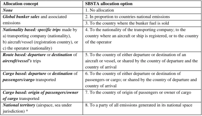
One of the reasons why international bunker emissions are not yet regulated is due to the unclear situation regarding who is responsible for these emissions. At the Conference of the Parties (COP) 1 in 1995 the UNFCCC Subsidiary Body for Scientific and Technological Advice (SBSTA) was requested to address the issue of allocation and control of emissions from international bunker fuels1_{. In 1996 the UNFCCC secretariat presented a paper at} SBSTA 4 that included eight allocation options for consideration by the countries (Table 1):

Table 1. Concepts and SBSTA allocation options for international marine and aviation bunker fuel emissions. Allocation concept SBSTA allocation option

None 1. No allocation

2. In proportion to countries national emissions Global bunker sales and associated

emissions 3. To the country where the bunker fuel is sold Nationality based: specific trips made by

a) transporting company (nationality), b) aircraft/vessel (registration country), or c) the operator (nationality)

4. To the nationality of the transporting company; to the country where an aircraft or ship is registered, or to the country of the operator

Route based: departure or destination of aircraft/vessel’s trips

5. To the country of either departure or destination of an aircraft or vessel, or shared by the country of departure and the country of arrival

Cargo based: departure or destination of passengers/cargo transported

6. To the country of either departure or destination of

passengers or cargo; or shared by the country of departure and country of arrival

Cargo based: origin of passengers/owner of cargo transported

7. To the country of origin of passengers or owner of cargo

National territory (airspace, sea under jurisdiction) *

8. To a party of all emissions generated in its national space

* E.g. territorial waters (12 mile zone), continental shelf, exclusive economic zone, national airspace.

1_{For a more elaborate background on the process within the UNFCCC, consult its website at:}

http://unfccc.int/adaptation/methodologies_for/vulnerability_and_adaptation/items/3416.php (consulted January 19th, 2006).

(14)

The analyses presented here focussed on two allocation options that seem to be the most practical in terms of a policy perspective:

• allocation according to nationality/registration (SBSTA Option 4): flag state of vessels, national airline’s aircraft activities; and

• allocation according to destination (SBSTA Option 6): imported goods and destination of passengers.

The first, nationality-based, option was selected for analysis as it fits in with the present regulatory regimes for international aviation and shipping within the framework of the International Civil Aviation Organisation (ICAO) and International Maritime Organisation (IMO), which are specialised agencies working with the UN to address policy issues on international transport. The second, cargo-based, option was selected since data is readily available on the import of goods by shipping route. At the regional level, this latter option is largely comparable to allocation according to the destination and departure of ships and airplanes, as intra-regional transit transport does not play a role at the regional level, while it does as at the national level. For Option 4 in aviation in this report the allocation of Option 5 (out-bound flights allocated to the country of departure and return flights to the country of destination) is used as a proxy, because no allocation was available for Option 4.

To explore the implications of allocating bunker emissions under a post-2012 regime for future commitments the Multi-Stage approach is chosen here, which is an incremental but rule-based approach for defining future emission abatement commitments. This approach assumes a gradual increase in both the number of parties taking on mitigation commitments and the level of commitment of the participating parties as the latter progress (graduate) through several stages in accordance to the rules for participation and differentiation (Berk and Den Elzen, 2001; Den Elzen et al., 2006c; 2006a). The Multi-Stage approach also appears to be the best method for fulfilling the various criteria (environmental, political, economic, technical, institutional) intrinsic to the multi-criteria evaluation of the approaches of Höhne et al. (2005) and Den Elzen and Berk (2003). The FAIR 2.1 model is used for the Multi-Stage analysis of regional emission allowances that are compatible with the long-term stabilisation of atmospheric greenhouse gas concentrations (Den Elzen and Lucas, 2005)2_.

2_{The FAIR model is designed for the quantitative exploration of a range of alternative climate regimes with the}

aim of differentiating between future commitments compatible with the long-term stabilisation of atmospheric greenhouse gas concentrations (Den Elzen and Lucas, 2005). The model uses the IPCC SRES baseline scenarios for population, gross national product (GDP) and GHG emissions (excluding bunker emissions) for 17 global regions [i.e. Canada, USA, OECD-Europe, Eastern Europe, the former Soviet Union (FSU), Oceania and Japan; Central America, South America, Northern Africa, Western Africa, Eastern Africa, Southern Africa, Middle East and Turkey, South Asia (including India), South-East Asia and East Asia (including China)] from the integrated climate assessment model IMAGE 2.3 (IMAGE-team, 2001), including the energy model TIMER 2.0 (Van Vuuren et al., 2006b). The historical GHG emissions are based on various data sets. The historical regional CO2 emissions from fossil fuel combustion and industrial sources are based on the IEA database (1970–2003)

(IEA, 2005) and the EDGAR database developed by MNP, TNO and JRC (Van Aardenne et al., 2001). The CO2

(15)

The baseline scenario used for the analysis in this report is the updated IMAGE/TIMER implementation of the Intergovernmental Panel on Climate Change (IPCC) SRES B2 scenario (Van Vuuren et al., 2006b) (hereafter referred to as the ‘B2 scenario’). The B2 scenario was selected since it is based on medium trend assumptions for population growth, economic growth and more general trends such as globalisation and technology development. In terms of quantification, the scenario roughly follows the reference scenario of the World Energy Outlook 2004 (IEA, 2004) and, after 2030, economic assumptions converge to the B2 trajectory (IMAGE-team, 2001). The population scenario is based on the UN Long-Term Medium Projection (UN, 2004).

The material presented in this report is structured as follows. Section 2 presents a baseline scenario for future international bunker emissions up to 2050 and regional responsibilities under various regional allocation options. Section 3 analyses various scenarios for dealing with the international bunker emissions in future international climate policy. Within this context, various options for regulating bunker emissions are explored, both as part of the Multi-Stage regime and separately on the basis of sector policies, as well as the implications for mitigation targets for the other sectors when international bunkers emissions are being abated or left unabated. In addition, the consequences of including the relatively high impact of non-CO2 emissions from aviation on radiative forcing in CO2-equivalent emissions from

international bunkers are evaluated. To assess the sectoral emission reduction potential we have developed CO2 mitigation scenarios based on the potential for energy efficiency

improvement and the introduction of biofuels. The conclusions drawn from these analyses are presented in section 4.

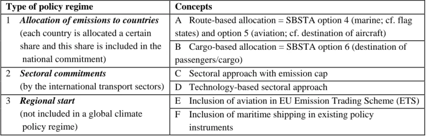
This analysis was made as part of a study reported by Faber et al. (2006), for which three different types of policy regimes have been explored, for each of which two concepts were elaborated:

Table 2. Concepts for the inclusion of bunker fuel emissions in climate policy. Type of policy regime Concepts

A Route-based allocation = SBSTA option 4 (marine; cf. flag states) and option 5 (aviation; cf. destination of aircraft) 1 Allocation of emissions to countries

(each country is allocated a certain share and this share is included in the national commitment)

B Cargo-based allocation = SBSTA option 6 (destination of passengers/cargo)

C Sectoral approach with emission cap 2 Sectoral commitments

(by the international transport sectors) D Technology-based sectoral approach

E Inclusion of aviation in EU Emission Trading Scheme (ETS) 3 Regional start

(not included in a global climate policy regime)

F Inclusion of maritime shipping in existing policy instruments

the Kyoto non-CO2 GHGs (CH4, N2O and the HCFCs, HFCs, PFCs and SF6), other halocarbons (e.g. CFCs,

HCFCs), sulphur dioxide (SO2) and the ozone precursors (NOx CO and VOC) are based on the EDGAR

(16)

(17)

2 Future projections of international marine and

aviation emissions

The projection and allocation of emissions requires, firstly, the determination of the emissions in the starting year for the scenarios; secondly, a model to estimate the

development of emissions over time; thirdly, an allocation of fuel consumption to countries. Each of these elements will be briefly discussed in this chapter. The differences in historical emissions estimates are discussed in more detail in text boxes, and details on the construction of the marine scenario are provided in the Appendix A. Historical CO2 emissions from

international shipping and aviation are surrounded by large uncertainties. For this reason, this report have estimated the emissions using two different methods – the top-down method based on national fuel sales statistics and the bottom-up method based on aircraft and

shipping characteristics (specific fuel consumption, etcetera) and their statistics (numbers and length of voyage). Both approaches have advantages and disadvantages (see Boxes 1 and 2).

2.1 International marine transport scenario

Very few source-specific scenarios exist for the emissions of international shipping. Although the emissions scenarios by Eyring et al. (2005b) are very detailed, they focus primarily on NOx emissions and other non-CO2 compounds and pay little attention to specific fuel

consumption and the trend in specific fuel consumption over time. Also, these scenarios do not provide a regional split in their emission projections.

With respect to international shipping, which in some studies is considered to be equivalent to ‘ocean-going ships’, different top-down and bottom-up data sets on historical fuel

consumption and CO2 emissions exist. While the principal causes of differences between

these data sets are known – for example, a significant fraction of domestic shipping may be included in the bottom-up estimates, as explained in Box 1 – it is currently not possible to implement precise corrections in either of the data sets. Consequently, the regional emissions scenarios presented here, which are based on IEA data for global total emissions in 2000 minus an amount estimated by Corbett and Köhler (2003) for military fuel use, should be considered to be a fair estimate and, as such, to be sufficiently accurate for analysing how the allocation options work out in practice.

Therefore, for the reasons discussed above we chose to develop a Baseline (trend) scenario, which is in line with the baseline B2 scenario (medium scenario) and which is based on historical data on the capacity per ship type in Dead Weight Tonnes (DWT) of tankers, bulk carriers, container ships, general cargo, among others, from the United Nations Conference on Trade and Development (UNCTAD, 2006b) . The following assumptions are made:

• The specific fuel consumption per DWT per major ship type remains constant over time (as suggested by historical data; see Appendix A);

(18)

• The historical fuel consumption trends were determined per type of shipping using DWT capacity per region and the definitions below;

• The regional 2000–2030 growth trends are based on historical regional capacity growth trends in the 1985–2003 period and linear extrapolation of the growth trend in the 2020s for the 2030–2050 period (with a few exceptions in cases of extreme high growth rates).

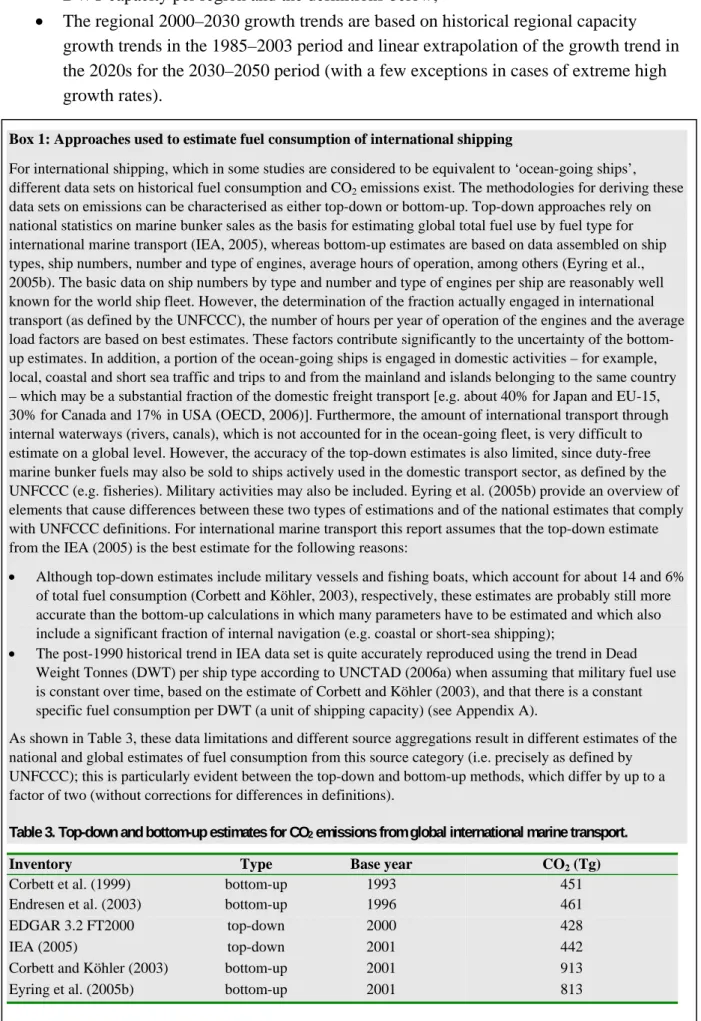
Box 1: Approaches used to estimate fuel consumption of international shipping

For international shipping, which in some studies are considered to be equivalent to ‘ocean-going ships’, different data sets on historical fuel consumption and CO2 emissions exist. The methodologies for deriving these

data sets on emissions can be characterised as either top-down or bottom-up. Top-down approaches rely on national statistics on marine bunker sales as the basis for estimating global total fuel use by fuel type for international marine transport (IEA, 2005), whereas bottom-up estimates are based on data assembled on ship types, ship numbers, number and type of engines, average hours of operation, among others (Eyring et al., 2005b). The basic data on ship numbers by type and number and type of engines per ship are reasonably well known for the world ship fleet. However, the determination of the fraction actually engaged in international transport (as defined by the UNFCCC), the number of hours per year of operation of the engines and the average load factors are based on best estimates. These factors contribute significantly to the uncertainty of the bottom-up estimates. In addition, a portion of the ocean-going ships is engaged in domestic activities – for example, local, coastal and short sea traffic and trips to and from the mainland and islands belonging to the same country – which may be a substantial fraction of the domestic freight transport [e.g. about 40% for Japan and EU-15, 30% for Canada and 17% in USA (OECD, 2006)]. Furthermore, the amount of international transport through internal waterways (rivers, canals), which is not accounted for in the ocean-going fleet, is very difficult to estimate on a global level. However, the accuracy of the top-down estimates is also limited, since duty-free marine bunker fuels may also be sold to ships actively used in the domestic transport sector, as defined by the UNFCCC (e.g. fisheries). Military activities may also be included. Eyring et al. (2005b) provide an overview of elements that cause differences between these two types of estimations and of the national estimates that comply with UNFCCC definitions. For international marine transport this report assumes that the top-down estimate from the IEA (2005) is the best estimate for the following reasons:

• Although top-down estimates include military vessels and fishing boats, which account for about 14 and 6% of total fuel consumption (Corbett and Köhler, 2003), respectively, these estimates are probably still more accurate than the bottom-up calculations in which many parameters have to be estimated and which also include a significant fraction of internal navigation (e.g. coastal or short-sea shipping);

• The post-1990 historical trend in IEA data set is quite accurately reproduced using the trend in Dead Weight Tonnes (DWT) per ship type according to UNCTAD (2006a) when assuming that military fuel use is constant over time, based on the estimate of Corbett and Köhler (2003), and that there is a constant specific fuel consumption per DWT (a unit of shipping capacity) (see Appendix A).

As shown in Table 3, these data limitations and different source aggregations result in different estimates of the national and global estimates of fuel consumption from this source category (i.e. precisely as defined by UNFCCC); this is particularly evident between the top-down and bottom-up methods, which differ by up to a factor of two (without corrections for differences in definitions).

Table 3. Top-down and bottom-up estimates for CO2 emissions from global international marine transport.

Inventory Type Base year CO2 (Tg)

Corbett et al. (1999) bottom-up 1993 451

Endresen et al. (2003) bottom-up 1996 461

EDGAR 3.2 FT2000 top-down 2000 428

IEA (2005) top-down 2001 442

Corbett and Köhler (2003) bottom-up 2001 913

(19)

In constructing the scenarios, two types of regional groupings/allocations were used for the historical trend and for projections of fuel consumption and CO2 emissions per ship type:

• As defined by flag of the country of registration corresponding with Option 4 of section 1: allocation according to the country where the ship is registered (hereafter

also designated as flag state);

• As defined by the import value per country (based on UNCTAD (2006a)) of goods that are generally transported by ships, using statistics for the major commodities per ship type to estimate the associated CO2 emissions; this corresponds with Option 6 of

section 1: allocation according to the country of destination of the cargo or passengers (hereafter also designated as imported goods).

Although both regional groupings result in somewhat different global total emission

projections, they are basically projections (extrapolations) of historical trends of capacity per ship type. The resulting differences in the two projections were removed by scaling both groupings to the same global total values. The reader is referred to Appendix A for more details on the historical trends and the methodology used for making the CO2 emission

projections.

When the historical trends of ship capacity are used for projecting CO2 emissions from 2000

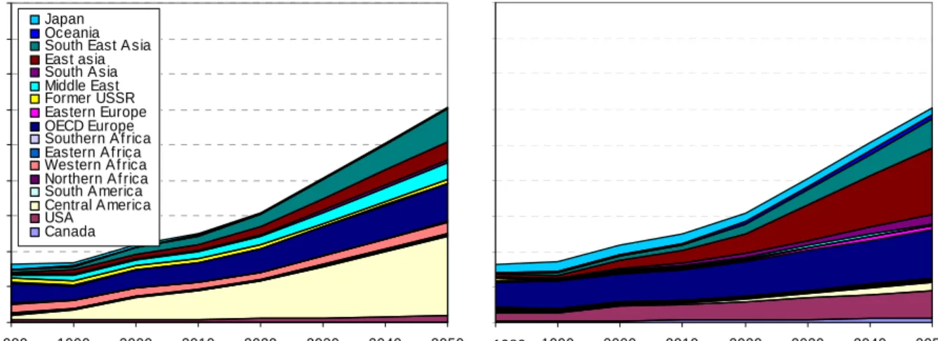
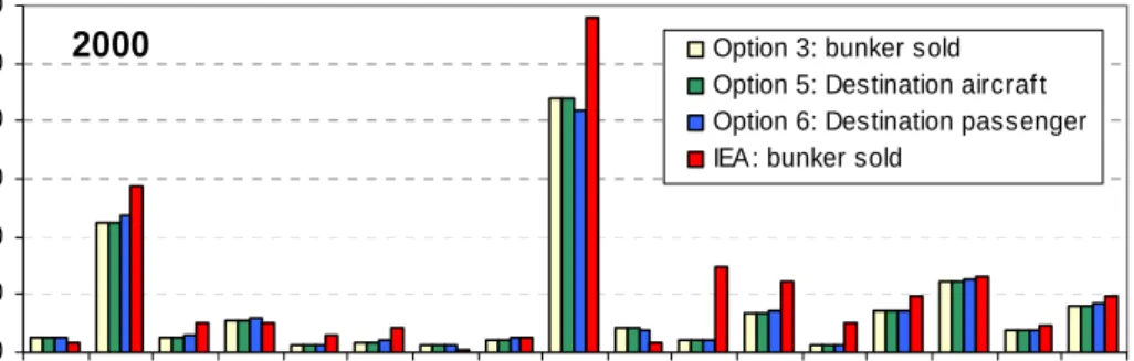
onwards, the result is a more than 40% increase in emissions by 2020 and an approximately 180% increase by 2050. As suggested by the differences in regional shares and trends in the registration of DWT capacity per flag country and by the value of imported goods (in USD), which are presented in Appendix A.1 (and illustrated in Figures A.1 and A.3), these different allocation methods also result in the development of highly different regionally allocated future CO2 emissions (Figure 1). Notable exceptions are OECD Europe and South-East Asia,

which show rather similar trends in both cases. When the global trends are compared with the four scenarios of Eyring et al. (2005b), the projected increases in the 2000–2020 period of 41–46% are very similar to the baseline (‘Business-As-Usual’) scenario. However, the projected increase in 2050 is somewhat higher than the largest projected increase in the Eyring scenarios, which is about 250%. These differences in regional allocations that

originate from the differences between Option 4 (allocation to flag nation, measured in DWT) and Option 6 (allocation to imported goods, expressed in USD) in the base year 2000

(Figure 2). The largest absolute differences are, once again, seen in the CO2 emissions from

Central America (i.e. the Caribbean) and Western Africa, with both of these regions showing much higher emissions in Option 4 (flag nations), and from the USA, OECD Europe, Middle East and Japan, all of which show much higher emissions in Option 6 (imported goods).

(20)

CO2 emissions from marine (option 4:flag state) 0 200 400 600 800 1000 1200 1400 1600 1800 1980 1990 2000 2010 2020 2030 2040 2050 Mt o n C O 2 Japan Oceania South East A sia East asia South A sia Middle East Former USSR Eastern Europe OECD Europe Southern A f rica Eastern A f rica Western A f rica Northern A f rica South A merica Central A merica USA Canada

CO2 emissions from marine (option 6:imported goods)

9801980 1990 2000 2010 2020 2030 2040 2050

Figure 1. Baseline (trend) scenario for regional CO2 emissions from marine transport using Option 4 (flag state)

(left) or Option 6 (imported goods) (right). Source: this study.

Inte rnational m arine e m is s ions (M tCO2) (e xcl. dom e s tic)

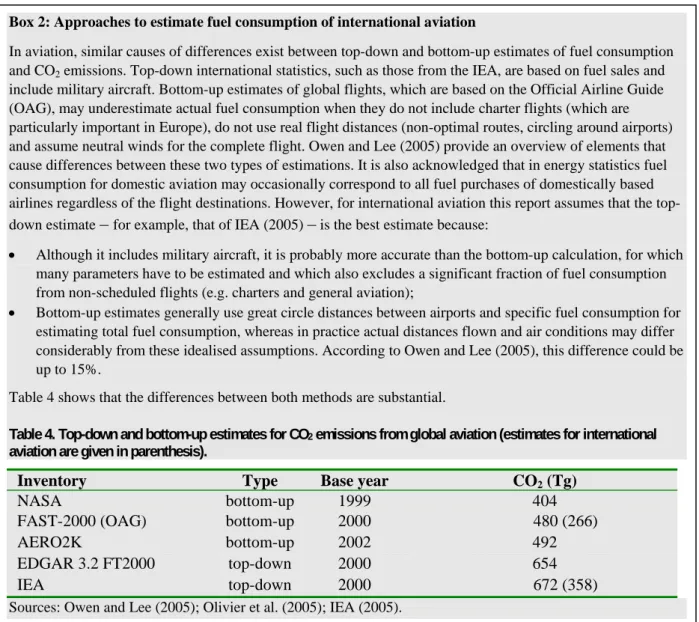
0 20 40 60 80 100 120 140 160 Cana da USA Cent ral A mer ica Sout h Am erica Northe rn Af rica We stern Afri ca Eas tern Afri ca Sout hern A frica OECD E uro pe Eas tern Eur ope Form er US SR Middl e E ast Sout h A sia East asi a Sout h E ast A sia Ocea nia Japa n Option 4: Flag state Option 6: Imported goods IEA : bunker sold

2000

Figure 2. The effect of different allocation options – Option 3 (bunker sold), Option 4 (flag state) or Option 6 (imported goods) – on international marine emissions based on data from UNCTAD (2006). The IEA bunker sales data are also depicted here for comparison purposes. Source: this study.

It should be noted that in contrast to most other emission sources, the allocation of maritime emissions to the flag countries where ships are registered is not very robust and may change significantly over time, since ship fleet owners may easily change the country of registration if national ship policies change substantially (e.g. administrative or tax regulations). In practice, however, the registration of most ships (in DWT capacity) is concentrated in a limited number of countries – the Bahamas, Panama, Liberia and Singapore in particular, but also Greece, Malta and USA. For some ship types, China, Hong Kong, Norway, Germany and the Netherlands can also be included in the list of most favourable flag states. However, since flag states play a key role in the implementation of IMO treaties, as do port and coastal states, and given the fact the interchanges of registration to flag states have been limited over

(21)

time, we have elaborated on the regional subdivision in the scenarios to identify any key specific differences between the two allocation options.

In addition, when considering inter-regional differences presented in this report one should keep in mind that regional totals are reported as the direct sum of imports by all countries within the regions and thus include intra-regional transport between countries. As such, net imports to the EU-25 as a region, for example, will actually be smaller than the figures presented here, which are the direct sum of imports of every member state. Moreover, the import value may include goods that are transported across countries using trucks (and rail and air). Nevertheless, the aggregation to regions using national import figures for goods that are mainly transported by ships provides a reasonably proxy for making comparisons.

2.2 International aviation baseline scenarios

Several emission scenarios for aviation are reviewed in IPCC (1999). However, only few data sources exist which have separated out the emissions from international aviation and

allocated historical fuel consumption and related CO2 emissions for international aviation

according to various options (see Box 2).

Owen and Lee (2005) calculated the amount of emissions from international aviation for the period 2005–2050 for the IPCC B2 scenario, which are used here. In their calculations, these authors used a very detailed bottom-up method, allocated to Parties, when working out allocation options 2, 3, 4, 5, 6 and 8 (section 1):

• Option 4: Nationality of airline – Under this option emissions were first estimated using the FAST model (see the description of Option 3a above). Emissions were then allocated according to the nationality of the airline. The feasibility of the alternative options under SBSTA Option 4 (allocation to the country in which the aircraft is registered or to the country from which the airline is operated) was considered to be uncertain and, consequently, allocation to nationality of the airline was selected. Although feasible for 2000, ownership of airlines is becoming progressively more complicated (designated hereafter also as national carrier).

• Option 5: Country of destination or departure of aircraft – Emissions were first calculated using the FAST model. The emissions from out-bound flights were then allocated to the country of departure and those from return flights to the country of destination. In other words, flight emissions were allocated to the country from which the aircraft ‘originally’ departed (designated hereafter also as destination aircraft). • Option 6: Country of departure or destination of passengers or cargo – This is an

alternative option in which emissions related to the journey of passengers or cargo are shared by the country of departure and the country of arrival. This implies that states have control over the emissions caused by the transport of cargo or passengers that enter or leave their country and, consequently, the control needed for this option resembles that needed for allocation Option 5. Emission trading and emission charges

(22)

could be designed to give states this control (designated hereafter also destination passenger).

Box 2: Approaches to estimate fuel consumption of international aviation

In aviation, similar causes of differences exist between top-down and bottom-up estimates of fuel consumption and CO2 emissions. Top-down international statistics, such as those from the IEA, are based on fuel sales and

include military aircraft. Bottom-up estimates of global flights, which are based on the Official Airline Guide (OAG), may underestimate actual fuel consumption when they do not include charter flights (which are particularly important in Europe), do not use real flight distances (non-optimal routes, circling around airports) and assume neutral winds for the complete flight. Owen and Lee (2005) provide an overview of elements that cause differences between these two types of estimations. It is also acknowledged that in energy statistics fuel consumption for domestic aviation may occasionally correspond to all fuel purchases of domestically based airlines regardless of the flight destinations. However, for international aviation this report assumes that the top-down estimate – for example, that of IEA (2005) – is the best estimate because:

• Although it includes military aircraft, it is probably more accurate than the bottom-up calculation, for which many parameters have to be estimated and which also excludes a significant fraction of fuel consumption from non-scheduled flights (e.g. charters and general aviation);

• Bottom-up estimates generally use great circle distances between airports and specific fuel consumption for estimating total fuel consumption, whereas in practice actual distances flown and air conditions may differ considerably from these idealised assumptions. According to Owen and Lee (2005), this difference could be up to 15%.

Table 4 shows that the differences between both methods are substantial.

Table 4. Top-down and bottom-up estimates for CO2 emissions from global aviation (estimates for international

aviation are given in parenthesis).

Inventory Type Base year CO2 (Tg)

NASA bottom-up 1999 404

FAST-2000 (OAG) bottom-up 2000 480 (266)

AERO2K bottom-up 2002 492

EDGAR 3.2 FT2000 top-down 2000 654

IEA top-down 2000 672 (358)

Sources: Owen and Lee (2005); Olivier et al. (2005); IEA (2005).

This report used the allocation of Owen and Lee’s Option 5 as proxy for Option 4 because no allocation was calculated for Option 4, and the ‘growth’ element of Option 4 is simply reflected in the FAST-2000 B2 scenario for Option 5 (D.S. Lee, personal communication, 2006). However, the scenario emissions were calculated using a bottom-up model requiring a large number of additional estimates, and these are likely to result in a considerable bias (see Box 2). Therefore, these emissions are scaled to match the international aviation CO2

emissions in 2000 estimated in IEA (2005). This scaling results in a global increase in 2000 of about 35% compared to the calculated FAST emissions. The largest absolute differences are seen in the emissions of OECD Europe (about 35%), the former USSR (a factor of 6 higher) and the USA (about 25% higher) (see Figure 3). Figure 3 also clearly shows that emissions of OECD Europe and the USA are much larger than those of the other regions presented. However, the emissions in the IEA data set allocated to the former USSR appear to be suspiciously high (D.S. Lee, personal communication, 2006), which reflects the

(23)

generally much higher uncertainty in the statistics for economies in transition. However, please note that the IEA total international bunker estimates also contains some uncertainty, as the IEA bunker data include military emissions, and countries do not always report their statistics in accordance to the definition requested.

Inte rnational aviation e m is s ions (M tCO2) (e xcl. dom e s tic)

0 20 40 60 80 100 120 Canada USA Centr al A mer ica South Ame rica Nort hern A frica Wes tern Afr ica Eas tern A fric a Sou ther n A frica OEC D E urope Easte rn E urope For mer USS R Middl e E ast Sou th As ia Eas t as ia Sout h E ast As ia Oceani a Japan Option 3: bunker sold

Option 5: Destination aircraf t Option 6: Destination passenger IEA : bunker sold

2000

Figure 3. The effect of three different allocation options on international aviation emissions: Option 3 (bunker sold), Option 4 (flag state) or Option 6 (imported goods). Emissions are based on data of Owen and Lee (2005). For comparison, IEA data are also depicted.

This report does not go into the specific outcomes of the different allocation methods here. The main conclusion of Owen and Lee (2005) is that the options favoured by SBSTA

(Options 3, 4, 5 and 6) are in close agreement3_{. This is also shown in Figure 3. Therefore, the} choice of one of these options over another does not appear to introduce a significant bias or distortion into the system (in contrast to clearly different systems, such as Options 2 and 8). However, in terms of some of the countries with relatively few emissions allocated, the allocation options can have a substantial impact on the amount of emissions allocated. The FAST B2 scenario is based on a scheduled air traffic projection by the Forecasting and Economic Support Group (FESG) of ICAO for revenue passenger kilometres up to 2020 and a logistic model of revenue passenger kilometres relating to GDP growth assumptions of the IPCC SRES B2 scenario. The GDP growth assumptions are an annual increase of 3.2% until 2010, followed by a decrease to 2.5% in the 2040–2050 period. Improvement in specific fuel consumption due to engine/airframe factors, which was not included in the FESG projections, were included based on historical trends; these amount to 1.3% per year for 2000–2010 and 1.0% per year for 2010–2020, whereas 0.5% per year was used for the 2020–2050 period

3_{This does not necessarily imply that this would remain so after an allocation method has been decided upon.}

Under some options, strategic actions to avoid inclusion under a stringent regime may be conceivable. This is analogous to the situation for sea shipping where vessels may be diverted to flag countries with less stringent commitments.

(24)

(Owen and Lee, 2005). More details on the regionalisation of the scenario (regional CAEP-6 forecasts up to 2020 and regional breakdowns up to 2050 according to the proportions in the CAEP-6 projection data) can also be found in this report.

The projection of the FAST B2 emission scenario for CO2 emissions from international

aviation from 2000 onwards shows an almost 100% increase in emissions by 2020 and an approximate 400% increase by 2050 (Figure 3). The FAST B2 emission scenario for total aviation results in about 2000 Tg CO2 for 2050, which is well within the range of

1500–5300 Tg CO2 projected by the group of scenarios for aviation presented in the IPCC

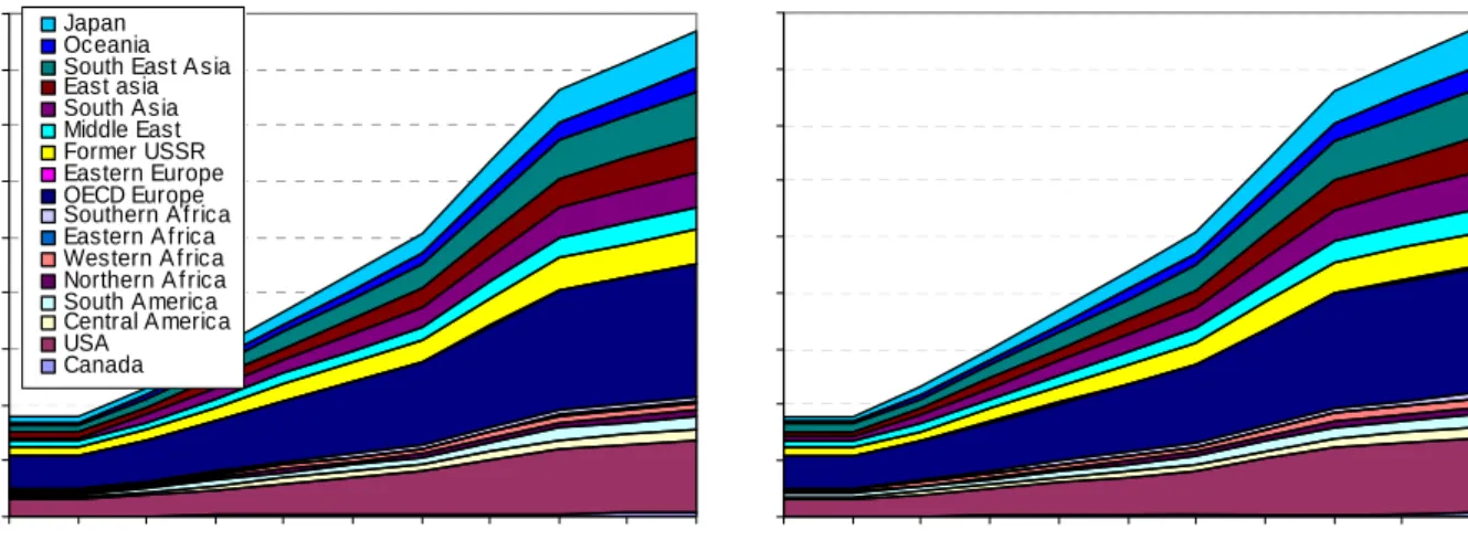
Special Report on Aviation (excluding the four most extreme, less probable ones). As suggested by the small differences in regional shares in 2000 (Figure 3), the allocation methods of Option 4 and Option 6 result in a rather similar development in terms of the regionally allocated CO2 emissions (Figure 4).

CO2 emissions from avation (option 5: dest.passenger)

0 200 400 600 800 1000 1200 1400 1600 1800 2000 2005 2010 2015 2020 2025 2030 2035 2040 2045 2050 Mt o n C O 2 Japan Oceania South East A sia East asia South A sia Middle East Former USSR Eastern Europe OECD Europe Southern A f rica Eastern A f rica Western A f rica Northern A f rica South A merica Central A merica USA Canada

CO2 emissions from avation (option 6: dest.airline)

2000 2005 2010 2015 2020 2025 2030 2035 2040 2045 20502000

Figure 4. Baseline B2 (trend) CO2 emissions scenario for international aviation allocated using Option 5

(destination/departure of passengers/cargo; used in analysis as proxy for Option 4) (left) or Option 6

(destination/departure of aircraft) (right) Source: historical data from IEA and scenario from Owen and Lee (2005).

However, we should recall the discussion on the accuracy of the national and global estimates of fuel consumption from this source category within the context of its exact definition by the UNFCCC (see Box 2), with particular reference to estimates based on top-down and bottom-up methods, which differ by bottom-up to a factor of two (without corrections for differences in definitions) (Table 4). Although the principal causes for these differences are known (e.g. a significant fraction of domestic aviation may be included in the bottom-up estimates), precise corrections in both types of data sets can not be made. Also note that the adjustment of the FAST emissions to IEA total international bunker estimates of 35% for fuel consumption that is not accounted for in the bottom-up FAST model also contains some uncertainty, as the IEA bunker data include military emissions, and reporting countries may not always report their statistics in accordance to the definition requested.

(25)

2.3 International bunker emissions

Without specific emission abatement, combined future bunker emissions from the aviation and maritime sectors are projected to grow in the baseline B2 (trend) scenario from about 800 Mt CO2 in 2000 to about 1350 Mt by 2020 and nearly 3000 Mt in 2050 (Figure 5.) This

is equivalent to an increase of approximately 70% in 2020 and 275% in 2050 compared to 2000. The aviation sector is responsible for most of this growth. While the shares of

international shipping and aviation in 2000 in terms of total CO2 bunker emissions are both

about 50%, in 2050 this has shifted to 40% for shipping versus 60% for aviation. However, when the Radiative Forcing Index (RFI) is applied to the CO2 emissions projection for

aviation – a measure to estimate and include the impact of specific non-CO2 emissions on

climate: the ratio of the total radiative forcing (RF) by all aviation emissions to that of CO2

from aviation alone, which is about 2.6 (see Box 5 in section 3.4.4) – the share of aviation in the bunker total increases from about two thirds in 2000 to 80% in 2050 (without specific abatement). The RFI value of 2.6 is based on IPCC (1999), which analyses the following contributions of aviation to radiative forcing: CO2, NOx, (via ozone changes and via methane

changes), contrails and stratospheric water vapour, sulphur and black carbon aerosols, cirrus cloud formation induced by aircraft emissions. In particular the contribution from NOx

emissions appeared significant; the impact on cirrus cloud formations is considered to be very uncertain. In a more recent study by Sausen et al. (2005) a new estimate of the RFI value was presented, which as somewhat lower than the IPCC estimate mainly because of a reduced estimate of the RF from contrails. However, they estimate the the potential range for the RF contribution from aviation induced cirrus clouds, which is not included in their estimate, much larger than the IPCC did.

international bunker CO2 emissions (option 4/5)

0 500 1000 1500 2000 2500 3000 3500 2000 2010 2020 2030 2040 2050 Mt o n C O 2 Japan Oceania South East A sia East asia South A sia Middle East Former USSR Eastern Europe OECD Europe Southern A f rica Eastern A f rica Western A f rica Northern A f rica South A merica Central A merica USA Canada

international bunker CO2 emissions (option 6)

20002000 2010 2020 2030 2040 2050

Figure 5. The international bunker emissions for the IPCC SRES baseline B2 scenario as constructed for this study for Option 4/5 [i.e. Option 4 for marine (flag state) and Option 5 for aviation (destination aircraft)] (left) and Option 6 marine and aviation (destination passenger/cargo) (right). Source: this study.

(26)

Fr action bunk e r e m is s ions in Bas e line B2 (e xcl. LUCF CO2) (in %) 0 2 4 6 8 10 12 14 16 18 20 Can ada _USA Cent ral Am erica Sout h Am erica Nor ther n Af rica We ster n A frica Eas tern A frica Sou ther n Af rica OEC D E urope East ern Europe Form er U SSR Middl e Eas t Sout h A sia Eas t as ia Sout h Ea st As ia Oceani a Japan Wo rld 2000-Option 4/5 2000-Option 6 2050-Option 4/5 2050-Option 6

Figure 6. Fraction of the bunker emissions in the overall regional and global anthropogenic CO2-equivalent

emissions for the B2 baseline scenario in 2000 (green) and 2050 (blue) for Option 4/5 (i.e. Option 4 for marine and Option 5 for aviation) and Option 6 marine and aviation). Source: MNP-FAIR model.

With respect to the regional projections, Figure 6 clearly shows that there are large differences for some regions depending on whether emissions are allocated according to nationality/flag or route/destination of passengers and goods. This is particularly true for Central America and Western Africa and, to a lesser extent, for Canada, Eastern Europe, Middle East, Japan (in the short term) and East Asia (China) (in the long term).

In summary, the main findings of this analysis are:

• Although the allocation of marine emissions to flag states is not very robust since the registration of most ships is concentrated in a limited number of countries and the country of registration may change easily over time, in practice the changes in registration to flag states over time have been limited during the past decades (see Appendix A).

• Using the Option 6 allocation (imported goods/aircraft destination), in 2050 the fraction of projected bunker CO2 emissions in total fossil CO2 emissions increases

substantially in OECD Europe, South-East Asia, Japan and Oceania from about 5% to shares of about 10%. The fraction in East Asia increases to about 5%, whereas the fraction in Western Africa decreases from over 10% to less than 5%.

• Using the Option 4/5 allocation (flag state/departing aircraft), in 2050 the fraction of projected bunker CO2 emissions in total fossil CO2 emissions increases substantially in

OECD Europe, Japan and Oceania to shares of between 5 and 15%, whereas the share of Western Africa decreases from over 25% to less than 10%. The fraction in Central America remains high (between 15 and 20%), whereas the fraction in Eastern Africa decreases from about 5% to about 1%.

• The flag state allocation of marine emissions, which plays a key role in the

implementation of IMO treaties, has a very large effect on the fraction of total bunker emissions to total fossil fuel-related CO2 emissions of a country. At the present time,

(27)

Singapore as well as Greece, Malta and USA. However, for some ship types, China, Hong Kong, Norway, Germany and the Netherlands are also among the most

favourable flag states. For those countries in particular, an Option 4 allocation of marine CO2 emissions would have a very large impact on their total national

greenhouse gas emissions.

• The shares of international shipping and aviation in total CO2 bunker emissions,

which at the present time are both about 50%, will shift in 2050 to 40% for shipping versus 60% for aviation. When the Radiative Forcing Index (RFI) for aviation is applied to include the non-CO2 contributions, the share of aviation in the bunker total

(28)

(29)

3 Mitigation scenarios

3.1 International aviation and marine emissions in climate

mitigation scenarios

In this section a quantitative approach is used to evaluate a number of scenarios in terms of how they deal with future bunker emissions. The first step will be to assess the implications of allowing bunker emissions to remain formally unallocated. In such a scenario, the bunker emissions would remain outside a future multi-lateral international climate regime, such as the Multi-Stage approach, and would grow unabated, as projected in chapter 2 of this report. This assessment will shed some light on both the additional mitigation burden for the

regulated emission sectors (mitigation penalty) as well as on how total emissions would exceed the emission caps for stabilisation if the bunker emissions are not compensated for (environmental penalty) (section 3.2.). Section 3.2 will also examine how actual regional emission allocations would develop if bunker emissions are accounted for in accordance with rules for allocating bunkers emissions (implicit allocations). Section 3.3 evaluates a number of cases in which bunker emissions are formally allocated and included in a future multi-lateral international climate regime, which at this time is the Multi-Stage approach. The aim of this evaluation is to explore the implications of different allocation rules for future

emission reduction/limitation targets for the Annex I and non-Annex I regions under a multi-stage regime by 2020 and 2050. Section 3.4 examines a number of cases in which bunker emissions are not included in a future multilateral international climate regime but are instead regulated directly within the sectors themselves (e.g. as part of coordinated policies and measures within the guidelines established by the IMO and ICAO). As such, the level of reductions in projected future bunker emissions is assessed that may be feasible up to 2050 and what this level would imply for the level of emissions reductions required for the (other) sectors regulated under the international climate regime. Table 5 provides an overview of all cases.

In all of the cases assessed here the medium growth baseline scenario – baseline B2 – is used as background for the analyses. The trend-based projections for the international shipping sector fit in well with this scenario. In addition, the policy cases use the global emission pathway (ceiling) for stabilising GHG emissions at 450 ppm CO2-equivalent, as described in

Den Elzen et al. (2006b). Finally, in those cases in which international bunker emissions are allocated, the allocation is carried out for both aviation and shipping emissions either

according to nationality/flag or according to destination/import. Although other combinations are possible in principle, these rules seem to be most consistent with a sovereignty-oriented approach or route-oriented approach to the allocation of responsibility for international

(30)

bunker emissions. All analyses were performed for 17 global regions, but for the purpose of clarity, the results are reported for ten aggregated groups of these regions. Given its high sensitivity to the allocation rules, Central America has been singled out as a separate region. Emissions up to 2010 are estimated as follows: it is assumed that Annex I countries

implement their Kyoto targets by 2010 and that all Non-Annex I countries follow their reference scenario until 2010.

Table 5. Overview of policy cases explored.

Case Climate policy Allocation of bunker emissions * Abatement of bunker emissions Compensation of bunker emissions 1. Baseline No No No No

2a. Mitigation penalty Yes No No Yes

2b. Environmental penalty Yes No No No

3a. Bunkers in climate regime (MS) Yes Yes Yes n.a.**

3b. Bunkers in climate regime unabated Yes Yes No Yes

4. Sector-based approach Yes No Yes n.a.**

* Including bunker emissions in regime ** Not applicable

Note: These cases are the subsequent graphs labelled as follows: 2a: compensation (excl.); 2b: no compensation (excl.); 3a: (incl.) reduced bunker; 3b: (incl.) unlimited bunker; 4: policy – compensation (excl.).

3.2 The implications of excluding bunker emissions from

future climate policy

3.2.1 The implications of emission reductions when compensating for the exclusion of bunker emissions in a Multi-Stage regime

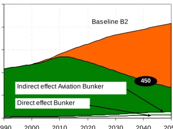
Figure 7 shows the global CO2-equivalent greenhouse gas emissions pathway for stabilising

concentrations in the atmosphere to be 450 ppm by 2100. The emissions pathway allows for overshooting; that is, the concentrations peak at 510 ppm before stabilising at 450 ppm at a later date. Global GHG emissions can still increase by about 20% above 1990 levels up to 2015 before they need to be reduced to 45% below 1990 levels by the middle of the century. If unabated, the share of international bunker emissions in allowable global emissions (including land use-related emissions) would increase from about 2% in 2000 to about 11% of the allowable emissions by 2050. Thus, over time, they would consume a substantial part of the allowable emissions. This does not include the additional impact of non-CO2 emissions

from aviation to radiative forcing, which enhances the impact by a factor of about 2.5 compared to CO2 only. The inclusion of all emissions affecting radiative forcing by aviation

would increase the share of international aviation emissions in allowable global emissions from 6 to 17%, thereby effectively doubling the share of total international bunker emissions to almost one quarter (21%).

(31)

Anthrop. CO2-eq emissions (incl. LUCF CO2) 0 20 40 60 80 100 1990 2000 2010 2020 2030 2040 2050 GtCO2/yr Baseline B2

Direct effect Bunker

Indirect effect Aviation Bunker 450

Figure 7. The share of (unabated) international bunker emissions(only the direct effects, used in the default calculations) (white area) in the B2 scenario (red area) compared to allowable emission levels for the stabilisation at 450 ppm CO2-equivalent concentrations (hereafter S450e emissions pathway) (green area). For comparison also

the additional indirect effect of the non-CO2 emissions is included (light-green). Source: adapted from Den Elzen et

al. (2006b).

In order to still comply with the global emission constraint for stabilising at 450 ppm, bunker emissions would need to be compensated for by more stringent emission targets for the other sectors regulated under the international climate regime. The ‘compensation (excl.)’ case (case 1) in Figures 8 and 9 shows the mitigation penalty of leaving international bunker emissions outside the climate regime and leaving them unabated, respectively. In the case shown, the international bunker emissions have been subtracted from the global emissions cap before the regional emission targets under the Multi-Stage regime were calculated (for details see Box 3 in section 3.3).

Evidently case 1 leads to higher reductions for all countries compared to the default case (not accounting for the bunker emissions in the calculations, as described in Den Elzen et al. (2006c)), as all countries need to compensate the increasing global bunker emissions. If the additional impact of non-CO2 emissions from aviation to radiative forcing is included, the

reductions for most of the Annex I countries become as high as 90% of the baseline emissions. For example, for the EU, the reductions compared to 1990 levels can become more than 20% in 2020 (instead of 12%) and 90% in 2050 (in stead of 75%).

Compared to the case in which bunker emissions are included (see Figure 10 below: case 3a), i.e. the case in which the global bunker emissions are not been subtracted from the global emissions cap, the results of the analysis show that compensating for increasing global bunker emissions leads in particular to higher emission reduction targets in both the short term (2020) and long term (2050) for the Annex I regions, such as North America and the EU. However, if the unabated bunker emissions are added to the regional emission targets according to the allocation rules of nationality and destination (import) – the ‘compensation

(32)

(incl.) case’ (case 2b) in Figures 8 and 9 – the de-facto emission allowances would be larger and thus their reduction targets lower (compare case 2b with case 1). Some regions would de-facto profit from excluding bunkers, while still compensating for them, such as Central America and South-East and East Asia, in particular. Compared to the inclusion of international bunkers in the Multi-Stage regime (case 3b) (see Figure 10), some regions would gain somewhat in the case of allocation to flag state, most notably the EU and Japan/Oceania, South-East Asia and, in particular, Central America. The differences seem small, but are likely to be more substantial at the national level (not shown here).

%-change compared to 1990-level in 2020

-30 -20 -10 0 10 20 30 Canada & USA Enlarged EU FSU Oceania &Japan Global 1.Compensation (excl.) - Option 4/5

1.Compensation (excl.) - Option 6 2a.No Compensation (incl.) - Option 4/5 2a.No Compensation (incl.) - Option 6 2b.Compensation (incl.) - Option 4/5 2b.Compensation (incl.) - Option 6 D f lt ( t ti b k )

450

0 20 40 60 80 100 120 140 Central America S. Amer& ME-Turk. Africa South Asia SE & E.Asia

-100 -90 -80 -70 -60 -50 -40 -30 -20 -10 0 Canada & USA Enlarged EU FSU Oceania &Japan Global

-50 0 50 100 150 200 250 Central America S. Amer& ME-Turk. Africa South Asia SE & E.Asia

Figure 8. Percentage change in the CO2-equivalent emission allowances relative to the 1990 emissions level for the

excluding bunkers case in 2025 and 2050 for the S450e emissions pathway for Option 4/5 (i.e. Option 4 for marine

and Option 5 for aviation) and Option 6 (marine and aviation). For comparison also the default case (not accounting for bunker emissions) is included. The lines included in the left column represent the outcomes when including the non-CO2 effects. Source: MNP-FAIR model.

3.2.2 The environmental implications of not compensating for excluding bunker emissions in a Multi-Stage regime

There is an environment penalty if there is no compensation for the unregulated increase in international bunker emissions in that emissions will then overshoot the emission pathway for meeting the 450 ppm stabilisation target. The ‘no-compensation case in Figure 8 shows that global emissions would exceed the global ceiling by about 8% by 2020 and 15% by 2050. The implications of this overshoot are that stabilisation at 450 ppm CO2-eq. would become

(33)

more difficult and probably result in an even larger initial overshoot of this target, even above the 510 peak that is assumed for the default pathway (see Den Elzen et al., 2006b).

Concurrently, the lack of compensation for the increase in bunker emissions would result in less stringent mitigation targets, particularly for the Annex I regions.

%-reduction comp. to baseline-level in 2020

-50 -45 -40 -35 -30 -25 -20 -15 -10 -5 0 Canada & USA Enlarged EU FSU Oceania &Japan Global 450 ppm

-50 -45 -40 -35 -30 -25 -20 -15 -10 -5 0 Central America S. Amer& ME-Turk. Africa South Asia SE & E.Asia 1.Compensation (excl.) - Option 4/5 1.Compensation (excl.) - Option 6 2a.No Compensation (incl.) - Option 4/5 2a.No Compensation (incl.) - Option 6 2b.Compensation (incl.) - Option 4/5 2b.Compensation (incl.) - Option 6 Default (not accounting bunker)

-100 -90 -80 -70 -60 -50 -40 -30 -20 -10 0 Canada & USA Enlarged EU FSU Oceania &Japan Global

-100 -90 -80 -70 -60 -50 -40 -30 -20 -10 0 Central America S.Amer& ME-Turk. Africa South Asia SE & E.Asia

Figure 9. Percentage change in the CO2-equivalent emission allowances relative to the B2 baseline scenario

emissions level for the case of excluding bunkers in 2025 and 2050 for the S450e emissions pathway for Option 4/5 (i.e. Option 4 for marine and Option 5 for aviation) and Option 6 (marine and aviation). For comparison also the default case (not accounting for bunker emissions) is included. Source: MNP-FAIR model.

(34)

Box 3. Multi-Stage approach

The Multi-Stage approach consists of a system in which the number of countries involved and their level of commitment increase gradually over time. It is based on pre-determined participation and differentiation rules that determine when a (non-Annex I) country moves (graduates) from one stage to the next and how its type and level of commitment changes. The aim of this system is to ensure that countries in similar economic,

developmental and environmental circumstances have comparable commitments under the climate regime. The Multi-Stage approach therefore results in an incremental evolution of the climate change regime. The approach was first developed by Gupta (1998) and subsequently elaborated (Berk and Den Elzen, (2001) Den Elzen, (2002) into a quantitative scheme for defining mitigation commitments under global emission pathways that are compatible with the UNFCCC objective of stabilising greenhouse gas concentrations. Höhne et al. (2005) extended the Multi-Stage approach with a pledging stage for Sustainable Development Policies and Measures, while Den Elzen et al. (2006c) developed a simpler version with some new types of participation thresholds. Here, the Multi-Stage approach is based on three consecutive stages for the commitments of non-Annex I regions beyond 2012. These are: Stage 1 – no commitment (baseline emissions); Stage 2 – emission limitation targets (intensity targets); Stage 3 – absolute reduction targets. In Stage 3, the total reduction effort to achieve the global emission pathway is shared among all participating regions on the basis of a burden-sharing key, which, in turn, is based on an equal weighting of greenhouse gas emissions per capita (in tCO2-equivalents per

capita) and per capita GDP income [in purchasing power parity (PPP) €1000 per capita] (e.g. Den Elzen et al., 2006a).4 Annex I regions are assumed to be in Stage 3 after 2012. Participation thresholds are used for the transitions between stages and are defined as the sum of per capita GDP income and per capita CO2-equivalent

emissions, thereby reflecting responsibility for climate change. Because it combines variables with different characteristics, this composite index should in principle be normalised and/or weighted. It happens, however, that one-to-one weighting combined with normalisation (to make it ‘unit-less’) produces satisfactory results. Current (2000) index values vary widely between countries, ranging from below 2 for Eastern and Western Africa, 4 for India and 8 for China to as high as 29 for the Enlarged-EU (EU-25) and 25 for the USA.

Table 6. Entry date in Stages 2 and 3 for the non-Annex I regions for the 450 ppm stabilisation scenario (e.g. Den Elzen et al., 2006a)

S450 Regions Central America South America Northern Africa Western Africa Eastern Africa Southern Africa Middle East South Asia East Asia South-East Asia Entry to Stage 2 ---- ---- ---- 2015 2065 2015 ---- 2015 ---- ----Entry to Stage 3 2015 2015 2020 >2050 >2050 2020 2015 2040 2015 2015

Source: MNP-FAIR model.

3.3 Bunker emissions in a Multi-Stage approach: the influence

of bunker allocation rules

The inclusion of international bunker emissions in the international climate regime will, in principle, provide more certainty in terms of the environmental effectiveness of the regime. In the Multi-Stage approach (see Box 3), only the emissions of those countries/regions in Stage 2 and 3 are regulated (see Table 6): countries in Stage 2 have emission limitation targets (intensity targets), while countries in Stage 3 adopt absolute reduction targets. The

4_{This leads to more balanced reduction targets for all regions compared to a burden-sharing key solely based on}