Evaluation of local learning rules in neural networks

(1)

Evaluation of local learning rules in neural networks

Academic year 2019-2020

Master of Science in Computer Science Engineering

Master's dissertation submitted in order to obtain the academic degree of Counsellor: Alexander Vandesompele

Supervisor: Prof. dr. ir. Joni Dambre Student number: 01404341

(2)

(3)

Evaluation of local learning rules in neural networks

Academic year 2019-2020

Master of Science in Computer Science Engineering

Master's dissertation submitted in order to obtain the academic degree of Counsellor: Alexander Vandesompele

Supervisor: Prof. dr. ir. Joni Dambre Student number: 01404341

(4)

Permission of use on loan

The author gives permission to make this master dissertation available for consultation and to copy parts of this master dissertation for personal use.

In all cases of other use, the copyright terms have to be respected, in particular with regard to the obligation to state explicitly the source when quoting results from this master dissertation.

(5)

Preface

First of all, I would like to thank my supervisor, prof. dr. ir. Joni Dambre, for the continuous support and guidance. Despite her busy schedule, she was always ready to respond to any questions with pragmatic feedback. Likewise, my counsellor, Alexander Vandesompele, offered valued insights for which I thank him. Without them this master’s dissertation would not have been possible.

I also want to express gratitude towards my parents for enabling and encouraging me to pursue a career in computer science.

Lastly, I want thank my friends for their support and witty comments, which kept me going whenever times were rough.

(6)

Abstract

Even though supervised learning with backpropagation surpasses humans on a multitude of tasks, it falls behind on cognitive capacity, flexibility and energy efficiency. The deep neural networks known today have come a long way since their origins in biologically inspired computing. However, since then the understanding of the human brain has also improved. A lot of the efficiency of learning is the result of self-organization: learning rules that work locally to adapt the network to the data it typically receives without any supervision or global reward. This work studies unsupervised local learning, based on Hebb’s idea that change in synaptic efficacy depends on the activity of the pre- and postsynaptic neuron only. In particular, the learning rule by Krotov and Hopfield is ex-amined as a method to train the hidden layers of artificial neural networks. To facilitate this analysis, a novel framework for systematic and thorough evaluation of local learning rules is proposed. It offers a high-level interface for both supervised and unsupervised local learning within a standard deep learning pipeline. Using the framework, the poten-tial and implications of Hebbian learning for image classification are highlighted. This work shows that supervised and Hebbian learned features are not simply interchangeable. Adaptations to conventional neural networks are needed to peer with the performance of backpropagation. Lastly, to show that Hebbian learning is not limited to shallow fully connected networks, a procedure to apply the Krotov-Hopfield learning rule to convolu-tional and multi-layer neural networks is proposed.

Keywords: Hebbian learning, local learning, machine learning, image classification, framework

(7)

1

Evaluation of local learning rules in neural networks

Jules Talloen

Supervisor: prof. dr. ir. Joni Dambre Counsellor: Alexander Vandesompele

Abstract—Neural networks were initially modeled after biological brains. However, the networks known today have come a long way since their origins in ’brain-inspired com-puting’. Supervised training with backpropagation excels at a wide variety of tasks but is both data- and power-hungry. This work studies unsupervised local learning, based on Hebb’s idea that change in synaptic efficacy depends on the activity of the pre- and postsynaptic neuron only. The Hebbian learning rule by Krotov and Hopfield is evaluated as a method to train the hidden layers of fully connected artificial neural networks for image classification. A framework for thorough and systematic evaluation of local learning rules in a standard deep learning pipeline is proposed. Using this framework, the potential and implications of Hebbian learned feature extractors are illustrated. In addition, an adaptation to the Krotov-Hopfield learning rule for convolutional and multi-layer networks is proposed.

Keywords— Hebbian learning, local learning, machine learning, image classification, framework

I. INTRODUCTION

The fascination with the human brain dates back thousands of years. With the advent of modern electronics, it was only logical to attempt to harness the cognitive abilities. Supervised learning with backpropagation produces impressive results on a diversity of tasks. In particular for vision, the early layers of convolutional neural networks (CNNs) learn to develop a multitude of informative features. Some of these closely resemble feature selectors in the early visual processing areas of higher animal brains [1]–[3]. Despite this resemblance, backpropagation is argued to be implausible from a biological perspective [4]–[6].

The deep neural networks known today have come a long way since their origins in ’brain-inspired computing’. However, since then the understanding of the human brain has also improved. One thing that remains certain is that the human brain is far more power- and data-efficient at computing than deep learning on digital computers. Although the mysteries of the human brain are far from solved, several learning mechanisms are well known. A lot of the efficiency of learning is the result of self-organization: learning rules that work locally to adapt the network to the data it typically receives without any supervision or global reward. In 1949, Hebb described the mechanism behind learning and memory

unsupervised. It turns out that these local learning rules are underexplored in artificial neural networks. The goal of this work is to evaluate learning rules, based on Hebb’s principles, for the artificial neural networks (ANNs) of today.

II. RELATED WORK

Hebbian learning is often applied to image tasks because of its close relation to visual processing in the brain of higher animals. As early as 1998, it was used to train a neural abstraction pyramid: a sequence of feature detectors with increasingly abstract representations of the image content [8], [9].

Hebbian learning has also successfully been applied to CNNs. Wadhwa et al. propose a neurologically plausible variant of competitive Hebbian learning as a foundation for bottom-up deep learning [10]. Their proposed algorithm produces sparse representations to be used in deep CNNs. Similarly, Bahroun et al. use Hebbian learning to acquire sparse multi-layer CNN features for image classification [11], [12]. Shinozaki proposes a biologically motivated learning method for deep CNNs [13]. He only trains the final layer with backpropagation and achieves state-of-the art performance as a biologically plausible method on the ImageNet dataset [14]. Illing et al. investigate the limits of image classification with biologically plausible, local learning rules in a network with one hidden layer [5]. They show that unsupervised learning does not lead to better performance compared to fixed random projections or Gabor filters for large hidden layers. Conversely, in this work, biological plausibility is not the main objective. Instead, the brain only acts as a source of inspiration rather than a set of restrictions.

This work starts from a recently proposed learning rule by Krotov and Hopfield [15]. Despite the locality constraint, their proposed algorithm achieves remarkable results on the image classification task. In parallel with this work, they published a follow-up paper that describes how their learning rule can be applied to CNNs [16].

III. SYNAPTIC PLASTICITY

In a neural network, each synapse is characterized by its strength or efficacy, denoted by a constant wij, commonly

referred to as the weight. This weight defines the magnitude of the postsynaptic neuron’s response to incoming signals. Synapses can be excitatory, wij > 0, or inhibitory, wij < 0.

(8)

2

and is the main underlying principle of learning and memory in the brain [17], [18].

In 1949, in an attempt to explain the process of synaptic plasticity between presynaptic neuron A and postsynaptic neuron B, Hebb stated the following:

When an axon of cell A is near enough to excite cell B and repeatedly or persistently takes part in firing it, some growth process or metabolic change takes place in one or both cells such that A’s efficiency, as one of the cells firing B, is increased [7].

The postulate is often rephrased as “neurons that fire together, wire together” [19]. This summarization should, however, not be taken too literally as it imposes no constraints on the direction of causation. The Hebbian theory claims that an increase in synaptic efficacy arises from a presynaptic neuron’s repeated and persistent stimulation of a postsynaptic neuron. This implies the presynaptic neuron should be active just before the postsynaptic neuron and the theory is hence asymmetric.

IV. HEBBIAN LEARNING

Hebb’s principle’s applicability is not limited to biological neural networks. From a mathematical perspective, Hebb’s postulate can be formulated as a mechanism to alter the weights of connections between neurons in an ANN. The weight between two neurons increases if they activate simulta-neously. Hebb’s postulate thus describes a procedure to adjust the parameters of a neural network. This process is called learning and accordingly, the postulate is called a learning rule.

(a) (b)

Fig. 1: (a) A connection with weight wijbetween pre- and postsynap-tic neuron, j and i. (b) Competition between neurons is introduced by adding inhibitory lateral connections (red arrows) between all neurons.

A. Hebb’s learning rule

Hebb’s learning rule describing the weight (wij) update

between a presynaptic neuron j and postsynaptic neuron i (Fig. 1a) is:

∆wij= ηyixj (1)

with η a positive multiplicative constant, sometimes called learning rate. This is the simplest Hebbian learning rule. Hebb’s rule reinforces the weight between pre- and postynaptic

η < 0, the learning rule is anti-Hebbian and weakens the weight between neurons with simultaneous pre- and postsy-naptic activity.

B. Normalization

Inherent in Hebb rule’s simplicity is instability, owing to the fact that weights will increase or decrease exponentially [20]. In biological neural networks this is not a problem because of natural limitations to the growth of synaptic strength. The synaptic strengths are regulated by homeostatic mechanisms stabilizing neuronal activity [21], [22]. In ANNs there is no such stability governing system by design. Hebb’s rule (1) creates a feedback loop by consistently reinforcing the weights between correlated neurons and impedes convergence. In order to limit exponential weight growth, the norm of the weight vector must be kept within bounds.

C. Inhibition

With multiple output neurons there is no system governing the learned patterns. A neuron’s incoming weights may con-verge to the same pattern as other neurons. It is desirable to extract more information than just a single pattern. In order to achieve this, more elaborate schemes are necessary to enforce distance among the learned patterns.

The acquired weights can be decorrelated by introducing inhibitory lateral connections between neurons [23]. This idea is schematically illustrated in Fig. 1b. Each neuron can now inhibit every other neuron (in the same layer) and competition is established. When a certain input pattern is applied, the neurons compete and only a few neurons respond strongly to the pattern, while the other neurons are inhibited. As a result, the ’winning’ neuron’s weights will move closer to the pattern. For other patterns, other neurons may ’win’ the competition, effectively forming neurons specialized for specific clusters of patterns. Ideally, each neuron converges to the center of mass of its cluster [24].

D. The Krotov-Hopfield learning rule

In 2019, Krotov and Hopfield proposed a biologically in-spired learning rule combining both normalization and lateral inhibition [15]. Their learning rule is rather unconventional, introducing a plethora of new variables, unseen in previous literature. Unfortunately, not all of these novel concepts are properly motivated or explained. Notwithstanding the lack of transparency, the rule shows remarkable performance with relatively low computational complexity.

Krotov et al. introduce their learning rule in the context of feedforward neural networks with a single hidden layer, consisting of M hidden neurons or units:

∆wij= g(rank(hwi, xii))(xj− hwi, xiiwij)

hwi, xii=

X

j

|wij|p−2wijxj (2)

(9)

3

smallest activation to M for the largest activation. Based on each unit’s rank µ, the activation function g is applied:

g(µ) =      1 µ = M −∆ µ = M − m 0 otherwise (3) with m a parameter that defines which hidden unit in the ranking is inhibited. Low values of m inhibit those units whose response to the applied pattern is strong. The function intro-duces competition between neurons via anti-Hebbian learning proportional to ∆.

Krotov et al. show that for ∆ = 0 and t → ∞ the weights wij (for a given hidden unit i) converge to a unit sphere:

|wi1|p+|wi2|p+|wi3|p+ ... +|wiN|p= 1 (4)

with N the number of input neurons. For 0 < ∆ < 0.6 the condition still holds for most hidden units.

V. SUPERVISED LEARNING WITHHEBBIAN LEARNING RULES

Because Hebbian learning is unsupervised, it can not be used to train a network for task specific outputs. During train-ing, the network summarizes as much information as possible from the input samples. The resulting weights are task-agnostic and the network is only able to extract useful features, which can then be used in later supervised stages. This is exactly what is done in the remainder of this work. Hebbian learning will be used to train the first layer(s) to perform task-agnostic feature extraction, after which backpropagation will be used to train the output layer for task dependent outputs.

Backpropagation also allows the Hebbian trained layers to be evaluated. Unlike backpropagation, Hebbian learning lacks clear performance metrics. The Hebbian layers will be evaluated in terms of the information content of the features they extract. If these features contain useful information, backpropagation should be able to use this information to tune the final layers and optimize the performance criterion.

VI. FRAMEWORK

Deep learning with backpropagation was greatly accelerated by frameworks such as TensorFlow [25] and PyTorch [26]. In particular, high level abstractions built on top of these frameworks, like Keras [27], allow rapid experimentation with-out worrying abwith-out the underlying complexity. Unfortunately, the Hebbian research community lacks such established tools. Popular deep learning frameworks revolve around training neural networks with backpropagation. Because of their focus on gradient based optimization, these frameworks are not di-rectly suitable for Hebbian learning. Nonetheless, TensorFlow and PyTorch offer many useful features, independent of the underlying training mechanism. For this reason, an entirely new framework for Hebbian learning would be redundant

A. Objectives

The goal of this work is to introduce a novel framework for thorough and systematic evaluation of Hebbian learning, or more generally, unsupervised local learning in the context of a standard PyTorch deep learning execution flow. The pro-posed framework is built to maximally support the following objectives:

• Data requirements analysis.

• Computational requirements analysis. • Performance analysis.

• Hyperparameter analysis. • Weights analysis.

B. Execution flow

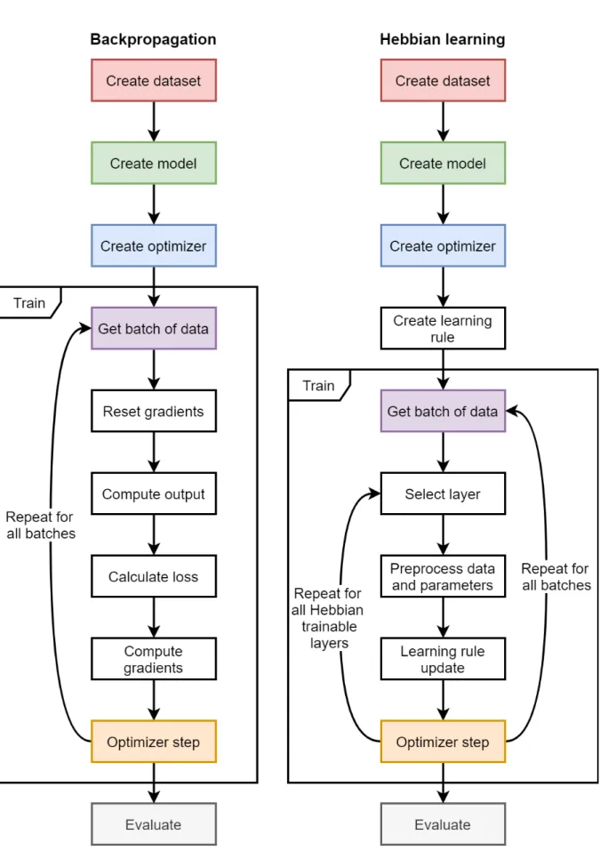
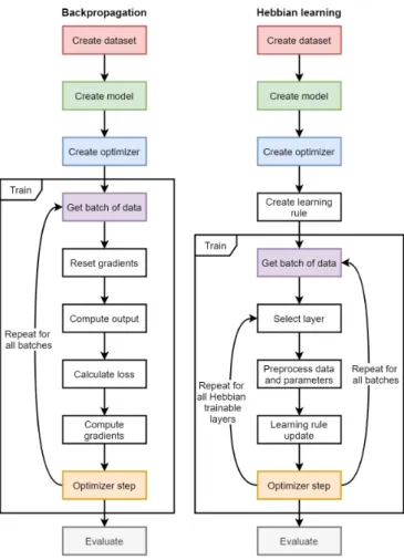
Hebbian learning introduces a new learning paradigm with an accompanying shift in execution flow. The comparison with backpropagation is made in Fig. 2. Both techniques first require the creation of a dataset, model and optimizer. In addition, Hebbian learning requires a local learning rule. Next, both methods execute the training algorithm and iterate over batches of data. Hebbian learning is local and trains each layer separately. In contrast, backpropagation trains all layers at once with a single forward and backward pass. The Hebbian paradigm thus introduces a second loop, iterating over the lay-ers. Once all Hebbian trainable layers are updated, the model continues onto the next batch of data. Upon completion of the epoch, both methods may execute an evaluation algorithm. The proposed framework implements both execution flows in a way that is transparent to the end user.

C. Core concepts

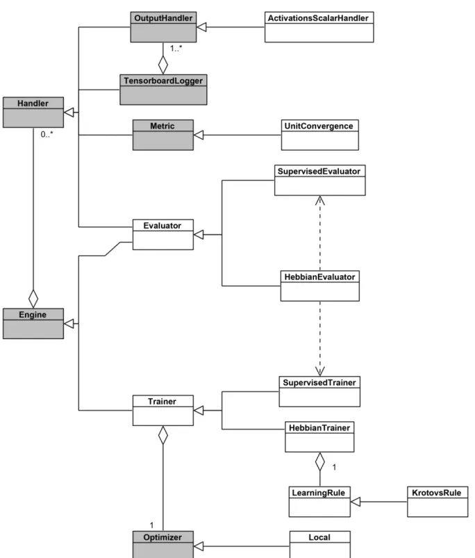
The core architecture of the framework is based on Py-Torch Ignite’s [28] Engine, Event and Handler classes. Everything revolves around the Engine, an abstraction that iterates over provided batches of data and executes a process-ing function. Two new Engine subclasses were introduced: the Trainer and Evaluator. The Trainer’s processing function updates the model’s parameters according to a spec-ified learning mechanism. In case of a HebbianTrainer, it is the Optimizer and LearningRule that determine how to modify the parameters in each iteration. On the other hand, the Evaluator’s processing function simply computes Metricson the validation data.

To facilitate flexible interfacing with the Engine’s ex-ecution flow, the PyTorch Ignite event system was put in place. Throughout an Engine’s run, Events are fired to which Handlers can respond. For example, for each epoch the EPOCH_STARTED and EPOCH_COMPLETED events are fired. By attaching event Handlers to the Engine for one or more Events, various powerful functionalities can be achieved. A Handler can be anything from an Evaluator to a Visualizer.

(10)

4

Fig. 2: A comparison of the execution flow of backpropagation and Hebbian learning. A single epoch is shown.

visual interfaces such as TensorBoard [29] are supported. Ten-sorBoard is a library for interactive visualization of machine learning experiments. It supports many types of visualizations including model graphs, histograms, distributions, embed-dings, images and scalar plots. These various visualizations and logs enable easy access to the information required to satisfy the framework’s analysis objectives.

D. Computational performance

Building upon PyTorch’s tensor backend, the proposed framework fully supports the compute unified device archi-tecture (CUDA®_{). CUDA}® _{is a parallel computing platform}

and programming model developed by NVIDIA for general computing on graphics processing units (GPUs) [30]. The proposed framework is more than 14 times faster compared to the original implementation [31] of the Krotov-Hopfield learning rule (2). The comparison is made in Table I.

Krotov et al. This work Time (seconds/epoch) 44 3

TABLE I: Time (in seconds) required per epoch for the numpy implementation (CPU only) by Krotov et al. [31] compared to this work (GPU accelerated).

VII. FULLY CONNECTED NETWORKS

Using the proposed framework, Hebbian learning can be applied in practice to train neural networks. This section covers fully connected feedforward neural networks with a single hidden layer. Fig. 3 illustrates the network with an input layer consisting of N = 784 neurons, a hidden layer consisting of M = 2000 neurons and an output layer with K = 10 neurons. The hidden layer’s initial weights are sampled from the standard normal distribution. The layer is then trained using the Krotov-Hopfield rule to perform task-agnostic feature extraction. Subsequently, the hidden layer is frozen and the final layer is trained with the supervised back-propagation rule, using the cross-entropy loss criterion and Adam optimizer [32]. While the cross-entropy loss criterion is used for backpropagation, accuracy will be the target metric. Bias units are only present in the final layer, because the Krotov-Hopfield rule does not specify a procedure to update them.

Fig. 3: A feedforward neural network with N input neurons xi, M hidden neurons hiand K output neurons yi.

The activation function for the hidden layer is a slightly unconventional adaptation of the rectified linear unit (ReLU) activation function. For the output layer, the softmax activation function is used:

hi= ReLU (wijxj)n= ReP U (wijxj, n)

yi= sof tmax(sijhj)

(5) with wijthe weights of the hidden layer and sijthe weights of

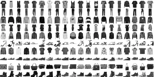
the final layer. In this work, the modified ReLU will be called a rectified polynomial unit (RePU), and n is a hyperparameter. Experiments will be conducted on 28×28 grayscale images from MNIST digits [33] and MNIST fashion [34]. Results are compared to a network of the same capacity trained end-to-end with backpropagation. No regularization is used in both the supervised and unsupervised stages.

A. Results

Krotov et al. report that their learning rule (2), when used to train the hidden layer, achieves 98.54% test accuracy on MNIST digits [15]. Training the same model with the optimal hyperparameters, using the novel framework, a slightly lower test score of 97.6% accuracy is achieved. The model trained end-to-end with backpropagation, converges to 98.55% test accuracy. Krotov et al. thus manage to match the performance of the backpropagation learning rule. Furthermore, there is less than 1% difference between the accuracy claimed by Krotov et

(11)

5

this work. The results on the train and test set are summarized in Table II.

Next, the model is analyzed on MNIST fashion. As seen in Table II, the train accuracy of Hebbian learning is significantly lower compared to end-to-end backpropagation. Furthermore, the Hebbian test accuracy is around 6% lower.

Train / test accuracy (%) MNIST digits MNIST fashion End-to-end backpropagation 100 / 98.55 99.57 / 90.86 Hebbian + backpropagation 99.18 / 97.6 87.65 / 85.32 TABLE II: Summary of the train and test accuracy of MNIST digits and MNIST fashion for end-to-end backpropagation compared to the Krotov-Hopfield Hebbian learning rule followed by backpropagation. B. Analysis

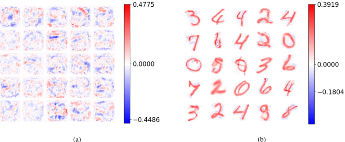
Fig. 4 and 5 show the weights of 25 randomly sampled hidden units for both the backpropagation (a) and Hebbian (b) network trained on MNIST digits and MNIST fashion respec-tively. The feature detectors achieved through backpropagation appear to be noisy and no intuitive patterns are present while the Hebbian detectors clearly show class prototype patterns.

For MNIST fashion, there is a clear performance gap between end-to-end backpropagation and Hebbian learning followed by backpropagation. Neural networks are typically trained with a single learning rule. With backpropagation as the most popular, years of research were dedicated to optimizing networks to achieve optimal results through back-propagation. Therefore, simply replacing the first layer with Hebbian weights and expecting everything else to work the same, is rather bold.

Fig. 6 compares the density histograms of the hidden layer activations for both learning methods. The distributions are clearly very different. The backpropagation hidden layer activations (Fig. 6a) roughly lie between -2.5 and 2.5 with the mean around 0. In contrast, the Hebbian activations (Fig. 6b) lie between -15 and 70 with a mean around 20. As result, an average of 1950 of the 2000 hidden units activate (RePU activation > 0) per input sample. In contrast, of the units trained with backpropagation, only 1350 activate on average. C. Batch normalization

As mentioned in Section VII, the hidden layer has no bias units in the Hebbian regime. When training the output layer with backpropagation, the model has no flexibility to shift the hidden layer’s outputs relative to the RePU non-linearity. Consequently, there is no way to limit the number of activating hidden units. As discussed in the previous section, almost all units activate and the output layer is flooded with information. To overcome this issue, the hidden layer outputs need scaling and bias that is trainable by backpropagation. Fortunately, this is what batch normalization does under the hood: it normalizes the inputs by re-centering and re-scaling [35]. By placing the batch normalization layer before the RePU activation, the supervised learning regime regains the power to scale and bias

The same network is trained again, now with batch normal-ization. The results are summarized in Table III. The Hebbian test accuracy is now only around 4% lower compared to end-to-end backpropagation. This is a ∼2% improvement over the same network without batch normalization.

Hebb Hebb + BN Backprop train accuracy (%) 87.65 89.67 99.57 test accuracy (%) 85.32 87.01 90.86

TABLE III: Summary of the train and test accuracy of the fully connected feedforward neural network on the MNIST fashion dataset. Hebbian learning followed by backpropagation (Hebb) without and with batch normalization (BN) compared to end-to-end backpropa-gation (Backprop).

D. Ablation study

The MNIST experiments are repeated with fixed standard normal initialized weights for the hidden layer. Only the weights of the final layer will trained, with backpropagation. The results are shown in Table IV. The network with random hidden weights achieves nearly the same performance as the fully trained network. Nonetheless, the Hebbian weights prove to be valuable with a 1% test accuracy increase.

Train / test accuracy (%) MNIST digits MNIST fashion Hebbian + backpropagation 99.18 /97.6 89.67 /87.01 Random + backpropagation 100 / 96.61 94.24 / 86.13 TABLE IV: Summary of the train and test accuracy of the fully connected feedforward neural network on the MNIST digits and fash-ion dataset. Hebbian learning for the first layer and backpropagatfash-ion for the final layer compared to a random initialized first layer and backpropagation for the final layer. MNIST digits experiments were performed without batch normalization.

VIII. CONVOLUTIONAL NEURAL NETWORKS Hebbian learning is not limited to fully connected networks. This section describes Hebbian learning with CNNs for image classification on MNIST fashion.

A. Convolution filter training

Unfortunately, the Krotov-Hopfield learning rule can not simply be fed the inputs and layer weights from a CNN in their current form. The dimensions of the input image and the convolution filters do not match, and the learning rule expects these to be the same. To overcome this dimension mismatch, image patches of the same dimensions as the convolution filters are extracted. The process is sketched in Fig. 8, for a 5 × 5 filter. The red squares represent the filter and the extracted image patch is shown for four filter positions. Now,

(12)

6

(a) (b)

Fig. 4: The incoming weights of 25 (out of 2000) randomly sampled hidden units trained end-to-end with backpropagation (a) and the Krotov-Hopfield learning rule (b) on the MNIST digits dataset.

(a) (b)

Fig. 5: The incoming weights of 25 (out of 2000) randomly sampled hidden units trained end-to-end with backpropagation (a) and the Krotov-Hopfield learning rule (b) on the MNIST fashion dataset.

(a) (b)

Fig. 6: Density histograms with 50 bins for the activation distribution of the hidden layer trained with backpropagation (a) compared to the Krotov-Hopfield rule (b).

(13)

7

Fig. 7: The layers of the fully connected network with batch normal-ization for the MNIST fashion setup. The batch normalnormal-ization layer follows the hidden layer and precedes the RePU activation layer.

Fig. 8: Image patches extracted from an MNIST fashion image. Four 5× 5 patches, extracted from four locations, are shown.

B. Setup

The layers are shown in Fig. 9. The model receives a 28×28 image with 1 color channel as input. Next is a convolutional layer with N = 400 filters, followed by a batch normalization, RePU and max pooling layer. Finally, the network flattens the convolutional features to a single dimension, before passing them to the fully connected output layer. The output layer has K = 10 units, one for each class. The convolutional layer is trained using the Krotov-Hopfield learning rule and both the batch normalization and fully connected output layer are trained using backpropagation.

Fig. 9: The layers of the CNN with a single hidden convolutional layer. The convolutional layer is Hebbian trained. The batch normal-ization and output layer are trained using backpropagation. The other layers do not contain trainable parameters.

C. Results

The results are summarized in Table V. With only 400 convolution filters, as opposed to the 2000 hidden units in the previous section, the network achieves 91.44% test accuracy, beating the previous results by ∼ 4.5%. Furthermore, the test accuracy of the network with Hebbian trained hidden layer is only 0.5% lower compared to end-to-end backpropagation! D. Multiple hidden layers

Hebb + backprop Backprop train accuracy (%) 98.64 99.98 test accuracy (%) 91.44 91.94

TABLE V: Summary of the train and test accuracy of the CNN on the MNIST fashion dataset. Hebbian learning followed by backprop-agation compared to end-to-end backpropbackprop-agation.

of the previous layer to construct powerful feature extractors. The proposed framework introduces Hebbian learning for multi-layer networks by mapping each layer to a different learning rule. In the simplest case, each layer is trained using the same learning rule but with different hyperparameters. The same learning rule and hyperparameters can not be used for each layer because the data distributions change upon passing through a layer. Each learning rule is to be optimized for the input distribution it receives.

IX. CONCLUSION AND DISCUSSION

This work began with an introduction to synaptic plasticity and Hebbian learning as the underlying principles of learning and memory in neural networks. In particular, the Krotov-Hopfield learning rule was introduced as a method to train the hidden layers of an ANN. Next, a novel framework for systematic and thorough evaluation of local learning rules was proposed. This is the first framework for Hebbian learning that can be incorporated in a standard deep learning pipeline. Using this framework, the Krotov-Hopfield learning rule was evalu-ated on MNIST digits and MNIST fashion. This work shows that Hebbian learned weights cannot simply be inserted into a classical backpropagation network without proper adaptations. Finally, an extension of the Krotov-Hopfield learning rule for convolutional and multi-layer networks was introduced. A procedure to train convolution filters on image patches was proposed.

With respect to task performance, the learning rule achieved similar results to end-to-end backpropagation on MNIST digits and MNIST fashion. This is at odds with the belief that early layer weights need to be tuned specifically for the task at hand. Moreover, a neural network with Hebbian weights is less susceptible to overfitting and generalizes better. However, with a large hidden layer, the Hebbian trained weights performed only slightly better compared to random weights. Further research is required towards backpropagation using Hebbian features on more challenging image datasets.

REFERENCES

[1] M. D. Zeiler and R. Fergus, “Visualizing and Understanding Convolutional Networks,” in Computer Vision – ECCV 2014 (D. Fleet, T. Pajdla, B. Schiele, and T. Tuytelaars, eds.), Lecture Notes in Computer Science, (Cham), pp. 818–833, Springer International Publishing, 2014.

[2] J. A. Bednar, “Hebbian Learning of the Statistical and Geomet-rical Structure of Visual Input,” in Neuromathematics of Vision (G. Citti and A. Sarti, eds.), Lecture Notes in Morphogenesis, pp. 335–366, Berlin, Heidelberg: Springer, 2014.

(14)

Unsuper-8

[4] S. Bartunov, A. Santoro, B. Richards, L. Marris, G. E. Hinton, and T. Lillicrap, “Assessing the Scalability of Biologically-Motivated Deep Learning Algorithms and Architectures,” in Ad-vances in Neural Information Processing Systems 31 (S. Bengio, H. Wallach, H. Larochelle, K. Grauman, N. Cesa-Bianchi, and R. Garnett, eds.), pp. 9368–9378, Curran Associates, Inc., 2018. [5] B. Illing, W. Gerstner, and J. Brea, “Biologically plausible deep learning — But how far can we go with shallow networks?,” Neural Networks, vol. 118, pp. 90–101, Oct. 2019.

[6] J. C. R. Whittington and R. Bogacz, “Theories of Error Back-Propagation in the Brain,” Trends in Cognitive Sciences, vol. 23, pp. 235–250, Mar. 2019.

[7] D. O. Hebb, The Organization of Behavior: A Neuropsycholog-ical Theory. Psychology Press, 1949.

[8] S. Behnke and R. Rojas, “Neural abstraction pyramid: a hi-erarchical image understanding architecture,” in 1998 IEEE International Joint Conference on Neural Networks Proceed-ings. IEEE World Congress on Computational Intelligence (Cat. No.98CH36227), vol. 2, pp. 820–825 vol.2, May 1998. [9] S. Behnke, “Hebbian learning and competition in the neural

abstraction pyramid,” in IJCNN’99. International Joint Confer-ence on Neural Networks. Proceedings (Cat. No.99CH36339), vol. 2, pp. 1356–1361 vol.2, July 1999.

[10] A. Wadhwa and U. Madhow, “Bottom-up Deep Learning using the Hebbian Principle,” p. 9, 2016.

[11] Y. Bahroun and A. Soltoggio, “Online Representation Learning with Single and Multi-layer Hebbian Networks for Image Clas-sification,” in Artificial Neural Networks and Machine Learning – ICANN 2017, Lecture Notes in Computer Science, (Cham), pp. 354–363, Springer International Publishing, 2017. [12] Y. Bahroun, E. Hunsicker, and A. Soltoggio, “Building Efficient

Deep Hebbian Networks for Image Classification Tasks,” in Artificial Neural Networks and Machine Learning – ICANN 2017 (A. Lintas, S. Rovetta, P. F. Verschure, and A. E. Villa, eds.), Lecture Notes in Computer Science, (Cham), pp. 364– 372, Springer International Publishing, 2017.

[13] T. Shinozaki, “Biologically-Motivated Deep Learning Method using Hierarchical Competitive Learning,” arXiv:2001.01121 [cs], Jan. 2020.

[14] J. Deng, W. Dong, R. Socher, L.-J. Li, K. Li, and L. Fei-Fei, “ImageNet: A Large-Scale Hierarchical Image Database,” in CVPR09, 2009.

[15] D. Krotov and J. J. Hopfield, “Unsupervised learning by com-peting hidden units,” Proceedings of the National Academy of Sciences, vol. 116, pp. 7723–7731, Apr. 2019.

[16] L. Grinberg, J. Hopfield, and D. Krotov, “Local Unsupervised Learning for Image Analysis,” arXiv:1908.08993 [cs, q-bio, stat], Aug. 2019.

[17] S. J. Martin, P. D. Grimwood, and R. G. M. Morris, “Synaptic Plasticity and Memory: An Evaluation of the Hypothesis,” Annual Review of Neuroscience, vol. 23, no. 1, pp. 649–711, 2000.

[18] W. C. Abraham, O. D. Jones, and D. L. Glanzman, “Is plasticity of synapses the mechanism of long-term memory storage?,” npj Science of Learning, vol. 4, pp. 1–10, July 2019.

[19] C. J. Shatz, “The Developing Brain,” Scientific American, vol. 267, no. 3, pp. 60–67, 1992.

[20] J. C. Pr´ıncipe, N. R. Euliano, and W. C. Lefebvre, “Hebbian Learning and Principal Component Analysis,” in Neural and adaptive systems: fundamentals through simulations, New York: Wiley, 1999.

[21] F. Zenke, G. Hennequin, and W. Gerstner, “Synaptic Plasticity in Neural Networks Needs Homeostasis with a Fast Rate Detector,” PLOS Computational Biology, vol. 9, p. e1003330,

[22] E. Marder and J.-M. Goaillard, “Variability, compensation and homeostasis in neuron and network function,” Nature Reviews Neuroscience, vol. 7, pp. 563–574, July 2006.

[23] P. F¨oldi´ak, “Forming sparse representations by local anti-Hebbian learning,” Biological Cybernetics, vol. 64, pp. 165– 170, Dec. 1990.

[24] W. Gerstner, W. M. Kistler, R. Naud, and L. Paninski, “Neuronal Dynamics: From Single Neurons to Networks and Models of Cognition.” https://neuronaldynamics.epfl.ch/online/index.html, 2014.

[25] “TensorFlow.” https://www.tensorflow.org/. [26] “PyTorch.” https://www.pytorch.org.

[27] F. Chollet, “Keras: The Python deep learning API.” https://keras. io/.

[28] V. Fomin, J. Anmol, S. Desroziers, Y. Kumar, J. Kriss, A. Te-jani, and E. Rippeth, “High-level library to help with training neural networks in pytorch.” https://github.com/pytorch/ignite. [29] “TensorBoard.” https://www.tensorflow.org/tensorboard. [30] “CUDA Zone.” https://developer.nvidia.com/cuda-zone, July

2017.

[31] D. Krotov, “DimaKrotov/Biological learning.” https://github. com/DimaKrotov/Biological Learning, Apr. 2020.

[32] D. P. Kingma and J. Ba, “Adam: A Method for Stochastic Optimization,” arXiv:1412.6980 [cs], Jan. 2017.

[33] Y. LeCun, C. Cortes, and C. Burges, “MNIST handwritten digit database, Yann LeCun, Corinna Cortes and Chris Burges.” [34] H. Xiao, K. Rasul, and R. Vollgraf, “Fashion-MNIST: a Novel

Image Dataset for Benchmarking Machine Learning Algo-rithms,” arXiv:1708.07747, Sept. 2017.

[35] S. Ioffe and C. Szegedy, “Batch Normalization: Accelerating Deep Network Training by Reducing Internal Covariate Shift,” arXiv:1502.03167 [cs], Mar. 2015.

(15)

4 A framework for Hebbian learning 42 4.1 Objectives . . . 42 4.2 Requirements . . . 43 4.3 Execution flow . . . 44 4.4 Core concepts . . . 45 4.4.1 Event system . . . 45 4.5 Trainers . . . 48 4.5.1 Hebbian trainer . . . 49 4.6 Optimizers . . . 51 4.7 Learning rules . . . 52 4.8 Handlers . . . 52 4.8.1 Metrics . . . 53 4.8.2 Evaluators . . . 53

4.8.3 Visualizers and loggers . . . 54

4.9 Computational performance . . . 56

4.9.1 Time profiling . . . 57

5 Hebbian learning in fully connected neural networks 60 5.1 General setup . . . 60

5.1.1 Datasets . . . 61

5.1.2 Model . . . 63

(17)

5.2 Reproduction of existing results with the novel framework . . . 65

5.2.1 MNIST digits . . . 65

5.2.2 CIFAR-10 . . . 68

5.3 Hyperparameter analysis on MNIST digits . . . 70

5.3.1 Inhibition hyperparameters . . . 71 5.3.2 The p hyperparameter . . . 74 5.3.3 Unit convergence . . . 74 5.3.4 The n hyperparameter . . . 76 5.4 MNIST fashion . . . 78 5.4.1 Setup . . . 79 5.4.2 Results . . . 80 5.4.3 Weight distribution . . . 81 5.4.4 Unit activations . . . 83 5.4.5 Batch normalization . . . 83

5.4.6 Results with batch normalization . . . 83

5.4.7 Activations after batch normalization . . . 85

5.4.8 The importance of inhibition . . . 86

5.5 Ablation study . . . 88

6 Hebbian learning in convolutional neural networks 92 6.1 Convolution filter training procedure . . . 92

6.2 Single hidden layer . . . 93

6.2.1 Model . . . 94

6.2.2 Setup . . . 94

6.2.3 Results . . . 95

6.2.4 Analysis . . . 96

6.3 Multiple hidden layers . . . 97

6.3.1 Model . . . 98

6.3.2 Setup . . . 99

6.3.3 Analysis . . . 100

6.3.4 Weight and activation distributions revisited . . . 100

(18)

7 Conclusion and future work 103 7.1 Conclusion . . . 103 7.2 Future work . . . 105

Bibliography 107

(19)

List of Figures

2.1 A typical neuron consist of 3 main parts: soma, dendrites and axon. A synapse connects one neuron’s axon to another neuron’s dendrites. Source: “The Synaptic Organization of the Brain” [1] . . . 9 2.2 Recordings of membrane potential aligned on the point of maximum

volt-age. These short electrical pulses, called actions potentials or spikes, show little variability in shape. Data courtesy of Maria Toledo-Rodriguez and Henry Markram [2] . . . 10 2.3 Two presynaptic neurons j = 1, 2 firing spikes at postsynaptic neuron i,

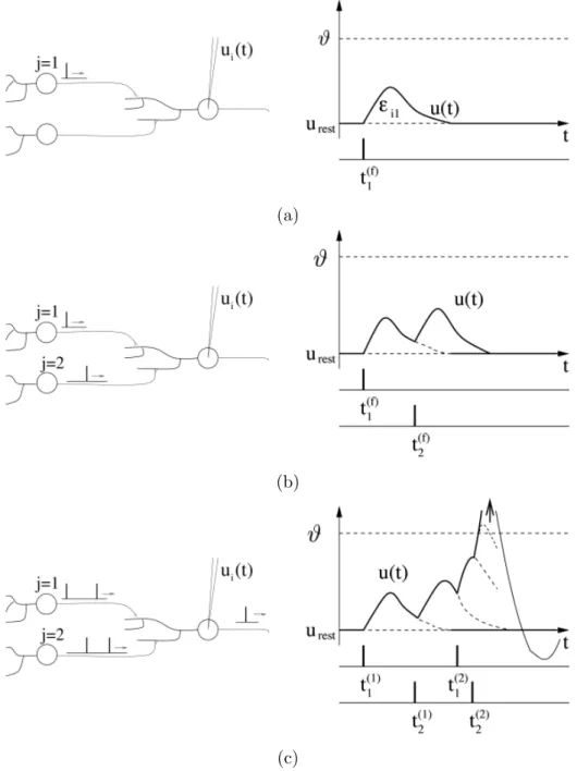
resulting in excitatory postsynaptic potentials (EPSPs). (a) The incom-ing spike evokes an EPSP. (b) The EPSPs of 2 temporally close spikes are added together. (c) Upon reaching the firing threshold ϑ, neuron i is excited and fires a spike. Source: “Neuronal Dynamics: From Single Neurons to Networks and Models of Cognition” [3] . . . 12 2.4 Hebbian learning. The change of the synaptic weight wij results from

the presynaptic neuron’s (j) repeated and persistent stimulation of the postsynaptic neuron (i). Other neurons (e.g. k) are not involved in the process of synaptic plasticity. Source: “Neuronal Dynamics: From Single Neurons to Networks and Models of Cognition” [3] . . . 14 2.5 A schematic drawing of a long-term potentiation (LTP) experiment

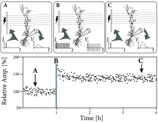
demon-strating Hebb’s postulate. (A) A small pulse is applied to the axonal end of the synapse, resulting in a postsynaptic potential but no action potential. (B) The synapse is repeatedly stimulated with pulses to invoke a postsy-naptic action potential or spike. (C) A significantly increased postsypostsy-naptic potential is detected in response to the same small pulse. The response amplitude relative to the initial amplitude is shown. At B, the amplitude is out of bounds. Source: “Neuronal Dynamics: From Single Neurons to Networks and Models of Cognition” [3] . . . 15

(20)

2.6 Spike-timing-dependent plasticity (STDP) adjusts synaptic efficacy based on the relative timing of a pre- and postsynaptic neuron’s spike. In case the postsynaptic neuron fires first, long-term depression (LTD) occurs whereas LTP occurs when the presynaptic neuron fires first. Source: “Synap-tic Modifications in Cultured Hippocampal Neurons: Dependence on Spike Timing, Synaptic Strength, and Postsynaptic Cell Type” [4] . . . 16 2.7 A perceptron with N inputs. Each input xj, j = 1, 2, ..., N is multiplied

with weight w1j and passed to the transfer function. The transfer function

sums the values and feeds them to the activation function, ϕ, which outputs the final activation. . . 18 2.8 A feedforward neural network with 2 hidden layers. All connections point

in the same direction. The input layer has 3 neurons, each hidden layer has 4 neurons and the output layer consists of 2 neurons. . . 19 2.9 The receptive field of hidden unit hi. The incoming weights of the unit are

reshaped to the input image dimensions (28_{× 28) to form a new image. .} 19 2.10 A Hopfield neural network with 4 units. The network has all-to-all

con-nectivity and symmetrical weights between units. . . 20 2.11 An example of a convolution operation. A 2 by 2 window, called kernel,

slides over the image. Here, three kernel positions are illustrated. Each pixel value is multiplied with the corresponding kernel value and summed to calculate a single output value. . . 22 2.12 The movement of a convolution filter. For an image with multiple color

channels, a kernel per channel is used. These kernels combined are called a filter. In this example there are 3 color channels (depth = 3). . . 22 2.13 Examples of low-level filters of a convolutional layer. Source: “ImageNet

Classification with Deep Convolutional Neural Networks” [5] . . . 23 2.14 A pooling layer can perform 2 types of pooling. Max pooling takes the

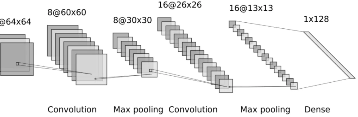
maximum value in its window (2 by 2 window here) and average pooling takes the average. . . 23 2.15 A neural network with multiple convolutional and pooling layers. Above

each layer, in ’A@B’, A stands for the amount of channels and B represents the image dimensions. The network ends in a dense or fully connected layer with 128 neurons. . . 24

(21)

3.1 Backpropagation in a neural network. The red path is one of the back-propagation paths, propagating error information from neuron y to neuron x. . . 27 3.2 A feedforward neural network. (a) In a local learning rule the weight

update for wij only uses local information from the pre- and postsynaptic

neuron, j and i. (b) A single linear neuron y1 with 3 incoming connections

from neurons xi, i = 1, 2, 3. . . 29

3.3 The dot product, y, ofx and w. For a linear neuron, assuming normalized inputs and weights, y measures the similarity between the inputx and the weightsw. . . 30 3.4 Illustration of the BCM rule’s activation function, φ. For postsynaptic

activity (denoted by νi) above the threshold νθ, LTP occurs, for

postsy-naptic activity below the threshold, LTD occurs and for activity below ν0

no change occurs. ν0 is typically set to 0. . . 33

3.5 Visualization of the incoming weights for 16 linear neurons trained with Oja’s rule (3.9). Due to lack of competition between neurons, they all converge to the same pattern, either positive or negative. . . 34 3.6 Competition between neurons in a layer is introduced by adding inhibitory

lateral connections (red arrows) between all neurons in that layer. . . 35 3.7 The pipeline for the Krotov-Hopfield learning rule. First, the inputs are

converted to input current Ii. Next, the hidden units (denoted by hµ)

compete for a positive activation according to (3.18). Upon convergence, the steady-state activities are fed through the activation function (3.19) to reach their final activation. Source: “Unsupervised learning by competing hidden units” [6] . . . 38 3.8 A comparison between the classical supervised and Hebbian learning

mech-anism. The lines at the bottom represent the flow of information. Each arrowhead represents weight updates. The supervised mechanism consists of a forward pass, to calculate the output, and a backward pass, to per-form backpropagation and update the weights. In contrast, the Hebbian paradigm only requires a single forward pass per layer. . . 40

4.1 A comparison of the execution flow of backpropagation and Hebbian learn-ing. A single epoch is shown. . . 46

(22)

4.2 UML class diagram of the core classes of the Hebbian framework. Every-thing revolves around the Engine. Trainers and Evaluators are special types of Engines, used to train and evaluate a model. The Evaluator is also a Handler to enable attachment to a Trainer. Handlers are used to perform various actions upon Events fired by the Engine. A broad range of functionality is covered by Handlers, ranging from metric computation to logging results to TensorBoard [7]. Classes shown in gray are part of PyTorch Ignite [8]. Not all classes are shown. . . 47 4.3 Events fired during the execution of an Engine. Upon running the Engine,

the STARTED event is triggered. Subsequently, for each epoch, EPOCH STARTED and EPOCH COMPLETED are fired at the start and end of the epoch respec-tively. Similarly, for each iteration the ITERATION STARTED and ITERATION COMPLETED events are fired. Finally, when the Engine has completed the specified amount of epochs, the COMPLETED event is triggered. . . 48 4.4 An example of the activations histogram (a) and distribution (b)

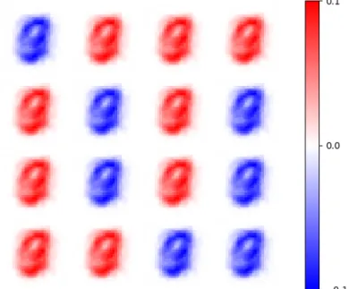
visu-alization in TensorBoard. For the histogram, the x-axis represents the activation values, the y-axis the counts and the depth represents the train-ing iterations. For the distribution plot, the x-axis represents the traintrain-ing iterations while the y-axis shows the activation value range. . . 55 4.5 An example of the weight (a) and unit convergence (b) visualization in

TensorBoard. Each weight image shows the incoming weights of a neuron, shaped to the input dimensions. The unit convergence plot shows the sum of the incoming weights of each neuron. . . 56

5.1 Some examples of the MNIST handwritten digits dataset. There are 10 classes consisting of handwritten digits from 0 to 9. . . 62 5.2 Some examples of the MNIST fashion articles dataset. There are 10 classes:

t-shirt/top, trouser, pullover, dress, coat, sandal, shirt, sneaker, bag and ankle boot. . . 62 5.3 Some examples of the CIFAR-10 dataset. There are 10 classes: airplane,

automobile, bird, cat, deer, dog, frog, horse, ship and truck . . . 63 5.4 A feedforward neural network with N input neurons xi, M hidden neurons

hi and K output neurons yi. . . 64

5.5 The rectified polynomial unit (RePU) activation function for various values of n. . . 64

(23)

5.6 Train and test accuracy curves for the fully connected neural network trained with end-to-end backpropagation compared to backpropagation for the final layer only, with a Hebbian learned hidden layer. . . 68 5.7 The patterns learned by the incoming weights of 25 (out of 2000) randomly

sampled hidden units trained end-to-end with backpropagation (a) and the Krotov-Hopfield learning rule (b) on the CIFAR-10 dataset. Source: “Unsupervised learning by competing hidden units” [6] . . . 69 5.8 The incoming weights of 25 (out of 2000) randomly sampled hidden units

trained end-to-end with backpropagation (a) and the Krotov-Hopfield learn-ing rule (b) on the MNIST digits dataset. . . 70 5.9 Examples of the incoming weights learned by hidden neurons. Each neuron

acts as a feature detector for a certain pattern. These patterns are not limited to the digit classes. Negative weights allow a feature detector to ’vote’ against other patterns. . . 72 5.10 Weights of hidden neurons learned with ∆ = 0.6, resulting in a few neurons

dominating and inhibiting the others to the point where no neuron learns a useful pattern. . . 72 5.11 An example of the incoming weights of a single hidden neuron trained with

overpowering inhibition. The neuron initially converged towards a useful pattern but was later strongly inhibited by other dominating units, causing it to lose its useful weights. . . 73 5.12 An example of the incoming weights of hidden neurons with ∆ = 0. All

weights are positive and each neuron is a feature detector for a single digit class. . . 73 5.13 The maximum weight value, of all connections towards the hidden layer,

in function of the p parameter. . . 75 5.14 An illustration of the Krotov-Hopfield normalization condition (3.17) for

2-dimensional inputs and various values of p. . . 75 5.15 Unit convergence (%) for five Hebbian training runs using different ∆ values. 76 5.16 The feature to prototype transition, in function of n, for dense

associa-tive memory (DAM) models trained on MNIST digits. Source: “Dense Associative Memory for Pattern Recognition” [9] . . . 78 5.17 The validation curves for different values of the RePU n hyperparameter.

The final layer of the network was trained with backpropagation, using Hebbian trained weights in the hidden layer. . . 79

(24)

5.18 The incoming weights of 25 (out of 2000) randomly sampled hidden units trained end-to-end with backpropagation (a) and the Krotov-Hopfield learn-ing rule (b) on the MNIST fashion dataset. . . 81 5.19 The incoming weights of 25 (out of 2000) randomly sampled hidden units

trained with the Krotov-Hopfield learning rule on the MNIST fashion dataset. 82 5.20 Density histograms with 50 bins for the weight distribution of the hidden

layer trained by backpropagation (a) and the Krotov-Hopfield rule (b). . 82 5.21 Density histograms with 50 bins for the activation distribution of the

hidden layer trained with backpropagation (a) compared to the Krotov-Hopfield rule (b) and the RePU layer trained with backpropagation (c) compared to the Krotov-Hopfield rule (d). . . 84 5.22 The layers of the fully connected network with batch normalization for the

MNIST fashion setup. The batch normalization layer follows the hidden layer and precedes the RePU activation layer. . . 85 5.23 Train and test accuracy curves for the fully connected neural network with

batch normalization. The network was trained on MNIST fashion with end-to-end backpropagation compared to backpropagation for the final layer only, with a Hebbian learned hidden layer. . . 86 5.24 Density histograms with 50 bins for the activation distribution of the batch

normalization layer trained with backpropagation (a) compared to the Krotov-Hopfield rule (b) and the RePU layer trained with backpropagation (c) compared to the Krotov-Hopfield rule (d). . . 87 5.25 Examples of hidden unit activations. The first image is the input, the

second image shows the weights of the activated hidden unit and the third image is the element-wise multiplication of the input and weights. White pixels represent zero. . . 89

6.1 Image patches extracted from an MNIST fashion image. Four 5_{×5 patches,} extracted from four locations, are shown. . . 93 6.2 The layers of the convolutional neural network (CNN) with a single hidden

convolutional layer. The convolutional layer is Hebbian trained. The batch normalization and output layer are trained with backpropagation. The other layers do not contain trainable parameters. . . 94

(25)

6.3 Train and test accuracy curves for the CNN trained on MNIST fashion with end-to-end backpropagation compared to backpropagation for the final layer only, with a Hebbian learned hidden layer. . . 96 6.4 The weights of 25 5_{× 5 convolution filters trained end-to-end with}

back-propagation (a) and the Krotov-Hopfield learning rule (b) on the MNIST fashion dataset. . . 97 6.5 The layers of the CNN with two hidden convolutional layers. The

convo-lutional layers are Hebbian trained. The batch normalization and output layer are trained with backpropagation. . . 98 6.6 The weights of 25 5_{× 5 convolution filters trained end-to-end with}

back-propagation (a) and the Krotov-Hopfield learning rule (b) on the MNIST fashion dataset. The filters are part of the second hidden convolutional layer from the architecture in Figure 6.5. . . 100 6.7 An example of 25 5_{×5 convolution filters trained with bad hyperparameters.101}

(26)

List of Tables

2.1 The relation between terminology in biological and artificial neural networks. 17

4.1 Time (in seconds) required per epoch for the numpy implementation (CPU only) by Krotov et al. [10] compared to this work (GPU accelerated). The proposed framework is more than 14 times faster. . . 57 4.2 Time comparison for Hebbian learning with the Krotov-Hopfield rule (3.16)

with the implementation by Krotov et al. [10] compared to this work’s implementation. Ranking time is reported both in milliseconds and as a percentage of the total execution time. . . 58

5.1 Summary of the train and test accuracy of the fully connected feedforward neural network on the MNIST digits dataset. Results claimed by Krotov et al. [6] compared to this work and end-to-end backpropagation. . . 68 5.2 Summary of the train and test accuracy claimed by Krotov et al. [6] on the

CIFAR-10 dataset [11]. ∗Krotov et al. do not mention the train accuracy at the epoch of the mentioned test accuracy (55.25%). They only mention the model was able to achieve 100% train accuracy after continuing to train it (overfitting on the train set). . . 69 5.3 A summary of the optimal hyperparameters for MNIST digits and MNIST

fashion. The MNIST fashion hyperparameters that changed with respect to those for MNIST digits are shown in bold. . . 80 5.4 Summary of the train and test accuracy of the fully connected feedforward

neural network on the MNIST fashion dataset. Hebbian learning followed by backpropagation compared to end-to-end backpropagation. . . 81 5.5 Summary of the train and test accuracy of the fully connected

feedfor-ward neural network on the MNIST fashion dataset. Hebbian learning followed by backpropagation (Hebb + backprop) with and without batch normalization (BN) compared to end-to-end backpropagation (Backprop). 85

(27)

5.6 Statistics of the hidden, batch normalization (BN) and RePU layer acti-vations in the network with and without batch normalization. . . 85 5.7 Summary of the train and test accuracy of the fully connected feedforward

neural network on the MNIST digits and fashion dataset. Hebbian learning for the first layer and backpropagation for the final layer compared to a random initialized first layer and backpropagation for the final layer. MNIST digits experiments were performed without batch normalization. 88 5.8 Summary of the accuracy on the test set of MNIST digits, MNIST fashion

and CIFAR-10 for end-to-end backpropagation compared to the Krotov-Hopfield Hebbian learning rule followed by backpropagation. The MNIST digits and CIFAR-10 experiments were performed without batch normal-ization. The MNIST fashion experiments were performed with batch nor-malization. . . 91

6.1 Summary of the train and test accuracy of the CNN on the MNIST fashion dataset. Hebbian learning followed by backpropagation compared to end-to-end backpropagation. . . 96 6.2 The results with the CNN reported by Grinberg et al. [12]. . . 98

(28)

List of abbreviations

AD automatic differentiation. 42

AI artificial intelligence. 8

ANN artificial neural network. 1–4, 6–8, 15–17, 24, 27–29, 31

CLI command line interface. 54

CNN convolutional neural network. xxi, xxii, xxiv, 2, 3, 5–7, 92–94, 96–98, 101–104

CPU central processing unit. 56–58, 104

CUDA® _{compute unified device architecture. 56–59, 106}

DAM dense associative memory. xx, 77, 78

ELM extreme learning machine. 88

EPSP excitatory postsynaptic potential. xvi, 11, 12

GMDH group method of data handling. 2

GPU graphics processing unit. 56–59, 104, 105

IPSP inhibitory postsynaptic potential. 11

LIF leaky integrate-and-fire. 1

LTD long-term depression. xvii, xviii, 13, 16, 33, 37

LTP long-term potentiation. xvi–xviii, 13–16, 33, 37

(29)

PCA principal component analysis. 4, 26, 32, 36

PSP postsynaptic potential. 11, 14

ReLU rectified linear unit. 21, 37, 63–65, 96

RePU rectified polynomial unit. xix–xxi, xxiv, 64, 65, 76–79, 83–85, 87, 90, 94, 96–98, 101, 104, 105

RNN recurrent neural networks. 16, 19, 20

SNN spiking neural network. 15

SOM self-organizing map. 6

STDP spike-timing-dependent plasticity. xvii, 15, 16

(30)

Chapter 1 Introduction

The fascination with the human brain dates back thousands of years. With the advent of modern electronics, it was only logical to attempt to harness the cognitive abilities. The development of models of neural networks supports a double objective. Firstly, the aim is to better understand the nervous system and secondly, to attempt to build information processing systems inspired by biological systems [13]. The first steps on the road to artificial neural networks (ANNs) were taken in 1943 when neurophysiologist, Warren McCulloch, and mathematician, Walter Pitts, wrote a paper describing how neurons might work [14]. They introduced a simple, formal neuron model based on electrical circuits. Reinforcing the idea of neurons and how they work was Donald Hebb’s book, The Organization of Behaviour, written in 1949 [15]. Hebb introduced the idea that biological neural networks store information in the strength of their connections and hypothesized a learning mechanism based on the modification of these strengths. His description of neural plasticity, the ability of the brain to change continuously throughout an individual’s life, became known as Hebbian learning. Three years later, in 1952, Hodgkin and Huxley established dynamic equations, based on recordings in the giant squid axon, which model the firing and propagation of signals in biological neurons [16]. In line with their work, Uttley introduced the leaky integrate-and-fire (LIF) neuron [17]. The LIF model is simpler and more functional compared to the Hodgkin-Huxley model, which more precisely models the underlying electrophysiology. Both the Hodgkin-Huxley and leaky integrate-and-fire models are still used today.

As computers evolved in the 1950s, early models capturing the principles of human thought arose. Farley and Clark first adopted computational machines, then called ’cal-culators’, to simulate a neural network based on Hebbian principles [18]. Not much later they were followed by Nathanial Rochester from the IBM research laboratories [19]. It

(31)

was at this point that traditional computing started prospering, leaving neural research in the background.

In 1958 Rosenblatt presented the perceptron, the oldest neural network still in use today [20]. The perceptron computes a weighted sum of its inputs and passes it on to a threshold function. This function returns one of two possible values as output. A few years later, in 1965, the first feedforward multi-layer networks were introduced [21]. These were trained by the group method of data handling (GMDH) and were the first example of hierarchical representation learning in neural networks. Eventually, 1969 marked the fall of the single-layer perceptron, when Minsky et al. published a book highlighting the limitations of the perceptron [22]. The perceptron was only capable of performing binary classification on continuous inputs. Certain information processing tasks require stacking of perceptrons in various layers, but at the time the learning rules for these architectures were unknown.

Notwithstanding the GMDH networks, the neocognitron (1979) [23, 24] was perhaps the first network that truly deserved to be called ’deep’. In addition, it introduced convolutions in neural networks. These networks are today typically called convolutional neural networks (CNNs) or convnets. The CNN was based on neurophysiological insights from Hubel and Wiesel (1959, 1962) [25, 26]. They found simple and complex cells in the cat’s visual cortex that fire in response to certain visual sensory inputs, such as the orientation of edges. They also found that the complex cells are more spatially invariant than the simple cells. Their discoveries not only inspired the neocognitron but also later work on award-winning deep neural network architectures.

Somewhat in parallel with the development of ANN architectures, new learning meth-ods to optimize the parameters of these ANNs were being researched. Although the minimization of errors through gradient descent by iterating the chain rule has been dis-cussed since the early 1960s (e.g. [27–30])1_{, it was only used in neural network specific}

applications in 1981 by Werbos [32]. The method became known as backpropagation and was further popularized by LeCun (1981, 1988) [33, 34] and Parker (1985) [35]. In partic-ular, a paper in 1986 by Rumelhart, Hinton and Williams [36] significantly contributed to the adoption of backpropagation. The combination of ever larger neural networks and backpropagation led to great improvements in the field of ANNs [31]. Notably, CNNs trained with backpropagation achieved great performance on massive image datasets such as ImageNet [37] [5].

Even though modern computers surpass humans on a multitude of tasks, they fall

(32)

behind on cognitive capacity, flexibility and energy efficiency. The deep neural networks known today have come a long way since their origins in ’brain-inspired computing’. However, since then the understanding of the human brain has also improved. One thing that remains certain is that the human brain is far more power- and data-efficient at computing than deep learning on digital computers: it learns much faster (i.e., with far fewer labeled examples) and consumes orders of magnitude less power. Humans even learn to extract useful visual features without any supervision in the form of labels. In fact, as deep learning is used to address more and more difficult tasks, the gap is widening rather than shrinking. Already, the data-hungriness of deep learning is restricting its applicability to those who can collect massive amounts of data.

Although the mysteries of the human brain are far from solved, several learning mech-anisms are well known. A lot of the efficiency of learning is the result of self-organization: learning rules that work locally to adapt the network to the data it typically receives without any supervision or global reward. This brings us back to 1949, when Hebb de-scribed the mechanism behind learning and memory in the human brain [15]. Hebb’s learning rule only depends on local variables and thus operates unsupervised. It turns out that these local learning rules are underexplored in artificial neural networks. So far Hebb’s rule applicability, outside modeling biological systems, has been limited. Most notably was Hopfield’s contribution in 1982 [38]. He introduced, what is now known as Hopfield neural networks: a type of recurrent ANN serving as associative memory. He used Hebbian learning to train the network to store useful information. Now, the goal is to evaluate learning rules, based on Hebb’s principles, for the ANN architectures of today.

1.1 Related work

Supervised learning with backpropagation produces impressive results on a diversity of tasks. In particular for vision, the early layers of CNNs learn to develop receptive fields for a multitude of abstract features. Some of these closely resemble feature selectors in the early visual processing areas of higher animal brains [39–41]. Despite this resemblance, backpropagation is argued to be implausible from a biological perspective [42–44]. In biological neural networks, the synaptic strength between neurons is adjusted using only local information, i.e. the activity of the pre- and postsynaptic neuron. A large body of research is devoted to constructing biologically plausible approximations to backpropa-gation [45]. Examples include feedback alignment [46–48], target propabackpropa-gation [49],

(33)

equilib-rium propagation [50], predictive coding [51] and alternating minimization [52]. Biological plausibility is not the objective of this work. Instead, the brain only acts as a source of inspiration rather than a set of restrictions. The goal is to evaluate the applicability of biologically inspired local learning rules in feedforward ANNs.

1.1.1 Local learning

Although some of the previously mentioned implementations use local learning rules, they include top-down information propagation to adjust the weights of the lower layers in the neural network. In contrast, this work studies local learning rules which rely on local information only and are unaware of the output state of the network. Since no error in-formation is propagated along the network, these rules are unsupervised. Although other implementations exist [53–55], this work further restricts the space of local learning rules by imposing correlated pre- and postsynaptic activity as a synaptic reinforcement require-ment. Correlation based learning was first studied by Hebb [15] and is now commonly known as Hebbian learning.

1.1.2 Hebbian learning

According to Debrito et al., Hebbian learning lies at the basis of various successful unsu-pervised representation learning algorithms [56]. Moreover, they suggest these algorithms can be reformulated using Hebbian learning rules. Hebbian learning is most commonly used to perform some form of principal component analysis (PCA). Applications range from PCA in non-euclidean spaces [57] to PCA type learning in linear neural networks with inhibition [58]. Additionally, Hebbian learning proves to be valuable in more general dimensionality reduction applications [59]. For example, Dony et al. compare Hebbian methods for the mixture of principal components (MPC) task in the context of image compression [60]. However, the principal components do not always contain the most information. Schraudolph et al. use Hebbian-like learning rules for the detection of invariant structure in a given set of input patterns [61].

In addition to feedforward neural networks, Hebbian learning has successfully been ap-plied to Hopfield neural networks [62], associative memory systems [63] and self-organizing maps [64].

Some suggest that concurrent change rather than concurrent activity more accurately captures the correlation requirement for Hebbian learning [65, 66]. They propose dif-ferential Hebbian learning. Difdif-ferential Hebbian learning rules are able to update the

(34)

synapse by taking into account the temporal relation, captured with derivatives, between the neural events happening in the recent past.

Another approach to Hebbian learning is studied in [67–70]. They postulate that the Hebbian learning rules originate from a similarity matching objective. These, or any other, objective functions will not be considered in this work.

Image tasks

As previously mentioned, Hebbian learned image features have a close relation to the early visual processing areas in the brain of higher animals [39–41]. Sensory cerebral cortices self-organize to capture the statistical properties of the input, thereby achieving a useful representation of the external environment. For this reason, Hebbian learning is often applied to train feature extractors for image tasks. Additionally, image classification is a popular task to test the performance of learning procedures for neural networks. Relatively simple datasets such as MNIST [71,72] and CIFAR-10 [11] are commonly used as benchmarks. This section will briefly cover related work on Hebbian learning for image tasks.

As early as 1998, Behnke et al. suggested using Hebbian learning to train a neural abstraction pyramid: a sequence of feature detectors with increasingly abstract repre-sentations of the image content [73, 74]. Their approach included both normalization and competition via lateral inhibition, two techniques crucial to make Hebbian learning feasible.

In addition to positively reinforcing correlated pre- and postsynaptic activity, Falcon-bridge et al. suggest anti-Hebbian learning: reducing synaptic strength on correlated activity [75]. They train a network for sparse, independent linear component extraction and show that the extraction of sparse components is biologically plausible.

Hebbian learning has also successfully been applied to CNNs. Wadhwa et al. propose a neurologically plausible variant of competitive Hebbian learning as a foundation for bottom-up deep learning [76]. Their proposed algorithm produces sparse representations to be used in deep CNNs. Similarly, Bahroun et al. use both Hebbian and anti-Hebbian learning to acquire sparse multi-layer CNN features for image classification [77,78]. They use competition via lateral connections and a similarity matching objective function.

Further progress is made by Amato et al. with experiments on the optimal combi-nation of Hebbian learning and supervised learning [79]. They show that their Hebbian algorithm is best used to train only a few of the lower or higher layers of a CNN. The suggested approach uses a winner-take-all activation function: an extreme case of