Flux measurements of ammonia at the micrometeorological weather station in Wageningen, The Netherlands

NH

3

flux measurements at the

micrometeorological weather station

in Wageningen, The Netherlands

Letter report 680150004/2009

RIVM Letter report 680150004/2009

Flux measurements of ammonia at the

micro-meteorological weather station in Wageningen,

The Netherlands

R.J. Wichink Kruit A.P. Stolk

H. Volten W.A.J. van Pul

Contact:

R.J. Wichink Kruit

Centre for Environmental Monitoring (CMM)

National Institute for Public Health and the Environment (RIVM) Roy.Wichink.Kruit@rivm.nl

This research is carried out on behalf of the Ministry of Housing, Spatial Planning and the Environment, Directorate General for Environmental Protection (VROM/DGM), in the framework of Project M/680150 Ammoniak.

RIVM Letter report 680150004/2009

Fluxmetingen van ammoniak op een

micro-meteorologisch weerstation in Wageningen,

Nederland

R.J. Wichink Kruit A.P. Stolk

H. Volten W.A.J. van Pul

Contact:

R.J. Wichink Kruit

Centrum voor MilieuMonitoring (CMM)

Rijks Instituut voor Volkgezondheid en Milieu (RIVM) Roy.Wichink.Kruit@rivm.nl

Dit onderzoek werd verricht in opdracht van het ministerie van Volkshuisvesting, Ruimtelijke Ordening en Milieubeheer, Directoraat-Generaal Milieubeheer (VROM/DGM), in het kader van Project M/680150 Ammoniak.

© RIVM 2009

Parts of this publication may be reproduced, provided acknowledgement is given to the 'National Institute for Public Health and the Environment', along with the title and year of publication.

Rapport in het kort

Fluxmetingen van ammoniak op een micrometeorologisch weerstation in Wageningen, Nederland.

Agrarisch grasland neemt aanzienlijk minder ammoniak uit de atmosfeer op dan tot nu tot werd aangenomen. Daardoor zit er in de atmosfeer een hogere concentratie ammoniak. Dit blijkt uit metingen op een micrometeorologisch weerstation in Wageningen door het RIVM en de Wageningen Universiteit. De metingen zijn boven agrarisch grasland verricht, dat 25 procent van het landareaal in Nederland omvat. Voorheen werden de metingen vooral in natuurgebied uitgevoerd. De komende jaren worden de consequenties van de nieuwe metingen in kaart gebracht. De metingen worden bovendien gebruikt om het transportproces van ammoniak van of naar het oppervlak beter te beschrijven.

Dit rapport beschrijft de metingen die aan deze conclusie ten grondslag liggen. Het onderzoek is uitgevoerd in opdracht van het ministerie van VROM, dat met deze metingen meer inzicht in de opname van ammoniak door grasland wilde hebben om het zogeheten ammoniakgat te verklaren. Het ammoniakgat is het verschil tussen de gemeten en berekende hoeveelheid ammoniak in de lucht, en is mede door dit onderzoek niet meer significant.

Ammoniak komt voornamelijk in de atmosfeer terecht door verdamping uit mest in stallen en bij het uitrijden van mest over het land. De hoeveelheid ammoniak die planten en de bodem opnemen is van invloed op de hoeveelheid ammoniak in de atmosfeer.

Abstract

Flux measurements of ammonia from a micro-meteorological weather station in Wageningen, the Netherlands.

Agricultural grassland absorbs considerably less ammonia from the atmosphere than has been believed up until now. This means that there is a higher concentration of ammonia in the atmosphere. This can be concluded from measurements taken from a micro-meteorological weather station in Wageningen by researchers from the National Institute for Public Health and the Environment (RIVM) and Wageningen University. The measurements were taken above agricultural grassland that covers 25 percent of the total land area of the Netherlands. In the past, the measurements were taken especially in nature areas. The consequences of the new measurements will be documented in future years.

Moreover, the measurements will be used in particular, to describe the transport process of ammonia to or from the surface.

This report describes the measurements on which this conclusion has been based. Commissioned by the Ministry of Spatial Planning and the Environment (VROM), the study was conducted to gain more insight in the uptake of ammonia through grassland in order to explain the so-called ammonia gap in the Netherlands. The ammonia gap is the difference between the measured and the calculated amount of ammonia which (partly due to the results of this study) is no longer significant.

Ammonia enters the atmosphere especially through the process of evaporation from manure in animal stalls and when liquid manure is spread over the land. The amount of ammonia absorbed by plants and the soil influences the amount of ammonia in the atmosphere.

Contents

Summary 7

1 Introduction 9

2 Derivation of the flux 13

2.1 Basic theory 13

2.2 Gradient or flux-profile technique 15

2.3 Footprint analysis 17

3 Site description and instrumentation 19

3.1 Site description 19

3.2 Instrumentation 20

3.2.1 Meteorological instrumentation 20

3.2.2 Ammonia instrumentation 20

4 Error analysis 23

4.1 Systematic and random errors in the concentration 23

4.1.1 Laboratory comparison 23

4.1.2 Field comparison 27

4.2 Random error in the flux 29

4.3 Effects of systematic errors in concentration measurements on the flux 33

4.4 Summary uncertainties and concluding remarks 35

4.4.1 Errors in the concentration 35

4.4.2 Errors in the flux 35

5 Overview of NH3 flux measurements and derived variables 37

6 Discussion and Conclusion 47

Literature 51

Appendix A. Micrometeorological variables and instrumentation at the micro meteorological

observatory 'Haarweg' in Wageningen, The Netherlands 55

Summary

To improve the description of the dry deposition process, new measurements of ammonia fluxes over agricultural grassland have been carried out by the National Institute for Public Health and the Environment (RIVM) in cooperation with the department of Meteorology and Air Quality of Wageningen University. The measurements with the new measurement device, the Gradient Ammonia – High Accuracy – Monitor (GRAHAM; Wichink Kruit et al., 2007), started in June 2004 and ended in December 2006. The GRAHAM, the measurement technique, the measurement site, the uncertainties in the measurements and the measurements themselves are described in this report.

After correction for the known systematic errors in the concentration measurements, a relative random error in the concentration of 1.9% is found. The relative random error in the NH3 flux measurements

(mainly determined by the propagation of the random errors in the concentration measurements in the flux calculation) is on average 52% (with a median value of 31%). If we would not correct for the systematic errors in the concentration measurements (0.6%), we would have an average systematic error in the flux calculation of 18%. This means that the systematic error is relatively small compared to the random error of the flux measurements on an hourly basis.

The measurements showed that the surface resistance (Rc), in particular the cuticular resistance (Rw), to

uptake of ammonia was much larger than assumed in the DEPAC (deposition) module used in the OPS model of RIVM and PBL and the Lotos/Euros model of TNO, RIVM and PBL. The currently applied resistance parameterisations for the dry deposition of ammonia on agricultural grassland are mainly based on measurements over natural ecosystems or semi-natural grasslands in areas with low ambient ammonia concentrations. We have shown in this report that the relatively high background concentrations in this study lead to higher surface resistances (and consequently lower deposition velocities) over agricultural grassland in The Netherlands. This is in agreement with findings of higher Rw values for different vegetations in high background concentration areas in literature (Nemitz et al.,

2001).

The main conclusion of this report is that the dry deposition description in the DEPAC module should be updated according to the current knowledge.

This research project is part of the research carried out to explain the ammonia gap in the Netherlands (van Pul et al., 2008).

1

Introduction

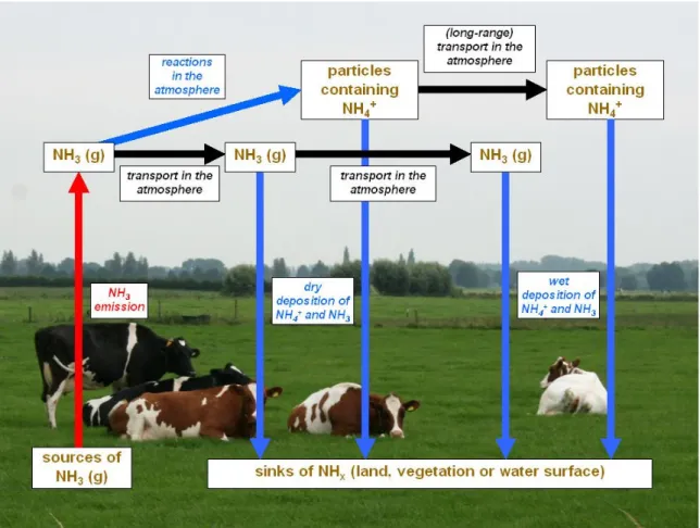
Several processes determine and influence the ammonia cycle in the atmosphere. Figure 1 shows the atmospheric processes that are important for ammonia. It starts with the emission of ammonia (red arrow in Figure 1). In The Netherlands, it was estimated that a total of 0.133 Tg of NH3 (= 133 kton)

was emitted in 2004 (Milieubalans, 2007), of which about 90% was of agricultural origin. For comparison, the yearly global emission was about 45 Tg NH3, of which about 67% was of agricultural

origin (Dentener and Crutzen, 1994).

Figure 1. Ammonia flows in the atmosphere.

Emission of NH3 is followed by atmospheric transport (black arrows in Figure 1). Transport and

dispersion of ammonia in the atmosphere occurs by mean wind and turbulence. There are three removal mechanisms for ammonia (blue arrows in Figure 1):

• The first one is chemical reactions that transform ammonia gas into particles containing ammonium. These particles have a longer lifetime than ammonia gas and are therefore transported over much larger distances.

• The second removal mechanism is dry deposition of NH3 and NH4+. NH3 and NH4+ are absorbed

by soil, vegetation and water surfaces. Dew plays an important role in the dry deposition process by enhanced surface wetness, because ammonia is well soluble in water.

• The third removal mechanism is wet deposition. Wet deposition is the transfer of NH3 and NH4+ to

the ground via precipitation, e.g. rain and snow. Wet deposition measurements are usually directly estimated from the measurement of the concentrations in precipitation and precipitation amount. One of the main items in the air pollution policy of the Dutch government is to reduce agricultural ammonia emissions. Over the last 30 years, ammonia has become widely recognized as a major atmospheric pollutant as a result of the effects of its deposition onto terrestrial and aquatic ecosystems and its influence on regional scale tropospheric chemistry (Grennfelt et al., 1994; Derwent et al., 1988). Deposition of reactive and reduced nitrogen species induces shifts in the nutrient balance that intensifies the eutrophication process. As a consequence, the existence of plant species changes and a loss of biodiversity occurs. Ammonia also contributes to the acidification of ecosystems through microbial oxidation (nitrification) in the soil. Therefore, the quantification of ammonia deposition is of great interest in assessing the effects of nitrogen loading to ecosystems.

To monitor the effectiveness of the measures taken by the government, The National Institute for Public Health and the Environment (RIVM, Bilthoven, The Netherlands) measures ammonia concentrations at 8 locations around the country and combines them with model calculations with an atmospheric transport model (OPS; Van Jaarsveld, 2004) to get a representative map of the ammonia concentrations and the ammonia deposition over the Netherlands.

The yearly averaged ammonia concentration observed by the monitoring network is plotted in Figure 2 (black solid line with squares). The figure also shows the total ammonia emissions by agricultural and other sources (bars), and the modelled ammonia concentration by the OPS model (red dashed line with triangles). A significant reduction in the emissions of ammonia is observed between 1993 (0.233 Tg yr

-1_{) and 2002 (0.139 Tg yr}-1_{). The measured yearly averaged ammonia concentration follows the}

decrease in ammonia emissions (from 10.6 µg m-3 in 1993 to 7.2 µg m-3 in 2002).

0.00 2.00 4.00 6.00 8.00 10.00 12.00 1993 1994 1995 1996 1997 1998 1999 2000 2001 2002 2003 2004 2005 2006 a m m oni a conc e n tr at ion (µ g m -3 ) 0 0.05 0.1 0.15 0.2 0.25 a m m oni a e m is si on ( Tg y r -1 )

total emissions measurements OPS model calculations

Figure 2. Emission, measured and modelled ammonia concentration from 1993 till 2006 (van Pul et al., 2008).

In general, the modelled concentrations (red dashed line with triangles) are lower than the measured concentrations (black solid line with squares). This absolute difference between the measured and modelled ammonia concentrations is about 30% and is called the 'ammonia gap'. Research on the 'ammonia gap' focuses on improving the emission factors from manure application (Berkhout et al., 2008) and improving the description of the dry deposition process. This report focuses on the latter. The dry deposition process is the most important removal process for ammonia from the atmosphere, however, it is usually not measured directly. The dry deposition flux is estimated as the product of the measured ammonia concentration (μg m-3) and a modelled deposition velocity (m s-1). The modelled deposition velocities at the ecosystem scale are based on process-based exchange models (Jakobsen et al., 1997). Much work has already been done to provide a mechanistic understanding of processes regulating the exchange (Sutton et al., 1993), however, there remain large uncertainties in these flux estimates, as there is a lack of validation by both laboratory and field measurements, especially over agricultural surfaces. However, for the mass balance (or concentration), ammonia exchange with especially agricultural grassland is very important as it covers about 25% of all land surface in The Netherlands.

To evaluate the existing parameterisation for the exchange of ammonia with agricultural grassland in the OPS model (Van Jaarsveld, 2004), measurements of ammonia fluxes over agricultural grassland have been carried out by RIVM in cooperation with the department of Meteorology and Air Quality of Wageningen University. The measurements of NH3 exchange started in June 2004 and ended in

December 2006. Non-fertilized grassland was chosen as a target land cover type as it is assumed to be useful as a background situation for all the (intensively) managed grasslands in The Netherlands. In this report the measurements above the grassland at the Haarweg, The Netherlands are presented. The first part of the report focuses on the theory and the methods applied. In Chapter 2 it is presented how the fluxes are derived from concentration measurements and how reliable data are selected from the dataset. Chapter 3 provides details about the measurement site and the instrumentation used to derive the ammonia fluxes. Chapter 4 presents an error analysis to give an impression of the errors in the concentration as well as in the flux measurements.

The second part of the report focuses on the results. In Chapter 5, an overview of the collected data and derived variables is shown. In Chapter 6, these results are discussed and placed in an international perspective.

The results of this research have been used in the report on the status of the ammonia gap (Van Pul et al., 2008)

2

Derivation of the flux

This chapter describes how the flux can be derived from concentration gradient and micrometeorological measurements. The gradient (or flux-profile) technique is commonly used in dry deposition studies and is based on the theory of turbulent flow of the atmospheric boundary layer. In applying this technique one should keep in mind that it is based on theory, which is only valid under certain conditions. If these conditions are not met this will lead to serious errors in the estimated flux.

2.1

Basic theory

Starting with the basic conservation equation of ammonia and expanding into mean (χ) and turbulent ( ) parts, the following equation is obtained (e.g. Stull, 1988): χ'

S x ' χ D x χ D x ' χ ' u x χ ' u x ' χ U x χ U t ' χ t χ 2 j 2 2 j 2 j j j j j j j j ₊ ∂ ∂ + ∂ ∂ = ∂ ∂ + ∂ ∂ + ∂ ∂ + ∂ ∂ + ∂ ∂ + ∂ ∂ ₍₁₎

where χ is the ammonia concentration, t is time, U is wind speed, x is the direction, u’ is wind speed fluctuation, D is the molecular diffusivity of ammonia, S is the net remaining source/sink term and j indicates the three spatial dimensions (x, y and z). Reynolds averaging and using the turbulent continuity equation (which puts the turbulent advection term into flux form (term III)) gives:

{

( ) ( ) ( )

{ V IV 2 2 2 2 2 2 III II I S z χ D y χ D x χ D z ' χ ' w y ' χ ' v x ' χ ' u z χ W y χ V x χ U t χ ₊ ∂ ∂ + ∂ ∂ + ∂ ∂ = ∂ ∂ + ∂ ∂ + ∂ ∂ + ∂ ∂ + ∂ ∂ + ∂ ∂ + ∂ ∂ 4 4 4 4 3 4 4 4 4 2 1 4 4 4 4 3 4 4 4 4 2 1 4 4 4 3 4 4 4 2 1 (2)

Term I represents the mean storage of ammonia (i.e. concentration change in time). Term II describes the advection of ammonia by the mean wind.

Term III represents the divergence of the ammonia flux. Term IV represents the mean molecular diffusion of ammonia.

Term V is the mean net body source (or sink) term for additional ammonia processes.

where U, V and W (and u, v and w) are the wind speed (fluctuations) in the x, y and z direction respectively.

To investigate the relative importance of each term in Equation 2, we scale all variables (a) with a typical scale (A) to make them dimensionless (â). We replace all variables according to â = a / A and Equation 2 is then rewritten as:

( )

( )

( )

3 2 1 4 4 4 4 4 4 4 4 3 4 4 4 4 4 4 4 4 2 1424 434 1424 434 1424 434 1 4 4 4 4 4 4 4 4 4 3 4 4 4 4 4 4 4 4 4 2 14 24 4 34 14 24 4 34 14 24 4 34 1 4 4 4 4 4 4 4 4 4 3 4 4 4 4 4 4 4 4 4 2 14 24 4 34 14 24 4 34 14 24 4 34 1 43 42 1 V χ IV IVC 2 2 2 IVB 2 2 2 IVA 2 2 2 III IIIC z IIIB y IIIA x II IIC z z IIB y y IIA x x I Sˆ S zˆ χˆ D Z DC yˆ χˆ D B DC xˆ χˆ D L DC zˆ ' χˆ ' wˆ Z c v yˆ ' χˆ ' vˆ B c v xˆ ' χˆ ' uˆ L c v zˆ χˆ Wˆ Z c Δ V yˆ χˆ Vˆ B c Δ V xˆ χˆ Uˆ L c Δ V tˆ χˆ t C ⎥ ⎥ ⎦ ⎤ ⎢ ⎢ ⎣ ⎡ + ⎥ ⎥ ⎦ ⎤ ⎢ ⎢ ⎣ ⎡ ∂ ∂ + ⎥ ⎥ ⎦ ⎤ ⎢ ⎢ ⎣ ⎡ ∂ ∂ + ⎥ ⎥ ⎦ ⎤ ⎢ ⎢ ⎣ ⎡ ∂ ∂ = ⎥ ⎥ ⎦ ⎤ ⎢ ⎢ ⎣ ⎡ ∂ ∂ + ⎥ ⎥ ⎦ ⎤ ⎢ ⎢ ⎣ ⎡ ∂ ∂ + ⎥ ⎥ ⎦ ⎤ ⎢ ⎢ ⎣ ⎡ ∂ ∂ + ⎥ ⎥ ⎦ ⎤ ⎢ ⎢ ⎣ ⎡ ∂ ∂ + ⎥ ⎥ ⎦ ⎤ ⎢ ⎢ ⎣ ⎡ ∂ ∂ + ⎥ ⎥ ⎦ ⎤ ⎢ ⎢ ⎣ ⎡ ∂ ∂ + ⎥ ⎥ ⎦ ⎤ ⎢ ⎢ ⎣ ⎡ ∂ ∂ (3)

Note that all factors between brackets are dimensionless and have values in the order of unity. The factors before the brackets are the scale variables needed to make the variables dimensionless. In Table 1 characteristic scales for all scale variables in Equation 3 are defined to investigate the relative importance of the individual terms.

Table 1. Characteristic scales and typical values used in scaling of the conservation equation of the concentration of ammonia.

Characteristic scale Symbol Typical value

concentration scale for NH3 C 10 µg m-3

concentration fluctuation scale for NH3 c 1 µg m-3

concentration difference scales for NH3 in the x, y

and z direction

Δcx, Δcy, Δcz 1, 1, 10 µg m-3

time scale of the mean concentration change of NH3 t 10000 s

mean wind speed scales of U, V and W Vx, Vy, Vz 5, 5, 0.001 m s-1

wind fluctuation scales in x, y and z direction vx, vy, vz 2, 2, 1 m s-1

length scales in the x, y and z direction L, B, Z 200, 200, 4 m

molecular diffusion coefficients for NH3 D 1.8 10-5 m2 s-1

If we fill in the typical values for the scales from Table 1 in Equation 3, we are able to make an estimation of the importance of each term:

I local time derivative:

001 . 0 10000 10 t C_{= =}

IIA and IIB advection by mean flow:

025 . 0 200 1 5 L c Δ V_{x x =} ⋅ ₌

IIC convection by mean flow:

0025 . 0 4 10 001 . 0 Z c Δ Vz z ₌ ⋅ ₌

IIIA and IIIB advection by turbulence:

01 . 0 200 1 2 L c v_{x =} ⋅ ₌

IIIC convection by turbulence:

25 . 0 4 1 1 Z c v_z ⋅ ₌ =

IVA and IVB molecular diffusion:

9 2 5 2 ₂₀₀ 4.5 10 10 8 . 1 10 L DC₌ ⋅ × − _{= ×} −

IVC molecular diffusion:

5 2 5 2 ₄ 1.125 10 10 8 . 1 10 Z DC₌ ⋅ × − _{= ×} −

As we do not have any information about the source/sink term (V), this term is ignored. However, it seems unlikely that sources and sinks are very strong within the surface layer and therefore this term is assumed to be relatively small compared to the other terms. We have to keep in mind that ignoring term V does not mean that there is no source or sink at the surface itself. We only ignore sources or sinks within the surface layer (e.g. chemical conversions within the surface layer).

We see that the largest term in Equation 3 is the convection by turbulence term (IIIC) and that all other terms are at least one order of magnitude smaller. Therefore, as an approximation, Equation 2 is

reduced to

( )

0 z ' χ ' w _≈ ∂ ∂

, which means that the flux is approximately constant with height. In other words, the flux that is measured at a certain height is approximately the same as the flux at the surface. The second largest term in Equation 3 is the advection by mean flow term (IIA and IIB). To be sure that the derived fluxes are not influenced by advection, we will use footprint analysis (Chapter 2.3) to exclude situations that advection might influence the flux measurements.

2.2

Gradient or flux-profile technique

At present, there exists no operational fast response sensor for ammonia. As a consequence, the ammonia fluctuations, χ', cannot be measured and the ammonia flux, Fχ =−

( )

w'χ' , can not be derived directly.

Therefore, we have to rely on another method to derive the ammonia flux: the gradient or flux-profile technique. This method relates the flux of ammonia to the vertical gradient of ammonia analogous to the description of molecular diffusion by Fick's law:

z χ K F_{χ χ} ∂ ∂ − = (4)

where ∂χ/∂z is the concentration gradient, i.e. the concentration difference, ∂χ, over a height difference, ∂z, and Kχ is the eddy diffusion coefficient for ammonia. Kχ is a property of the flow and depends

largely on turbulence in that flow.

Characteristic turbulence scales for the different scalar quantities are defined: a turbulence velocity scale, the so-called friction velocity:

4 1 2 2 ' w ' v ' w ' u u_∗ =⎜_⎝⎛ + ⎟_⎠⎞ (5a)

and a turbulence scale for the quantity of interest such as temperature, absolute humidity or in our case ammonia (χ), generally written as:

∗ ∗ =−w_u'χ'

χ (5b)

By combining Equation 5a and 5b, the ammonia flux is written as:

∗ ∗ − = u χ

Fχ (6)

The gradient in Equation 4 is made dimensionless through the flux-profile relationships (or stability functions) for ammonia (Φχ), which is assumed to be transported in the same way as heat (H) and

moisture (Q), e.g. Φχ(ζ) ≈ ΦH(ζ) ≈ ΦQ(ζ) (Dyer and Hicks, 1970; Businger et al., 1971; Webb, 1980):

( )

ζ Φ z U u kz m = ∂ ∂ ∗ (7a)

( )

ζ Φ

( )

ζ Φ z χ χ kz H χ ≈ = ∂ ∂ ∗ (7b)

where k is the von Karman's constant (=0.4). The dimensionless flux-profile relationships Φm and Φχ

are functions of the atmospheric stability parameter ζ = z/L, where L is the Obukhov length scale defined by:

' χ ' w u kg T L=− 3∗ (8)

Using Equation 4, 6 and 7, the eddy diffusion coefficient for ammonia is written as:

( )

ζ Φ z ku K χ χ = ∗ (9)

If we integrate Equation 7a over a height difference, z - z0,m, we obtain:

( )

⎟ ⎟ ⎠ ⎞ ⎜ ⎜ ⎝ ⎛ ⎟⎟ ⎠ ⎞ ⎜⎜ ⎝ ⎛ + ⎟ ⎠ ⎞ ⎜ ⎝ ⎛ − ⎟ ⎟ ⎠ ⎞ ⎜ ⎜ ⎝ ⎛ = − ≡ ∂ = ∂

∫

∗ ∗

∫

L z Ψ L z Ψ z z ln k u ) z ( U ) z ( U z kz ζ Φ u U 1 _{m m} 0,m m , 0 m , 0 z z m z z0,m 0,m (10a)

In a similar way Equation 7b is integrated over a height difference, z - z0,χ:

( )

( )

⎥ ⎥ ⎦ ⎤ ⎢ ⎢ ⎣ ⎡ ⎟⎟ ⎠ ⎞ ⎜⎜ ⎝ ⎛ + ⎟ ⎠ ⎞ ⎜ ⎝ ⎛ − ⎟ ⎟ ⎠ ⎞ ⎜ ⎜ ⎝ ⎛ = − ∗ L z Ψ L z Ψ z z ln k χ z χ z χ _{χ χ} 0,χ χ , 0 χ , 0 (10b)

where ψm(ζ) and ψχ(ζ) are the integrated stability functions, z0,m and z0,χ are the characteristic length

scales of the underlying surface for wind velocity, U, and ammonia, χ, respectively. They indicate the height above a virtual zero level at which the centre is located where the quantity is transmitted, absorbed or released. The z0,m, called the roughness length, is dependent on the roughness of the

surface. The z0,χ is mainly dependent on the vertical distribution of the sources or sinks of ammonia at

the surface.

Here, we use the integrated stability functions of Paulson (1970) and Dyer (1974) for unstable conditions (i.e. L < 0):

( )

( )

2 π x tan 2 2 x 1 ln 2 x 1 ln 2 ζ Ψ_m 2 − 1 + ⎥ ⎥ ⎦ ⎤ ⎢ ⎢ ⎣ ⎡ + + ⎥⎦ ⎤ ⎢⎣ ⎡ + = − _(11a)

( )

( )

⎥ ⎥ ⎦ ⎤ ⎢ ⎢ ⎣ ⎡ + = ≈ 2 x 1 ln 2 ζ Ψ ζ Ψ_{χ H} 2 (11b) where _x=

(

₁−_16ζ

)

14 with _ζ=_{z L}

and the integrated stability functions of Beljaars and Holtslag (1991) for stable conditions (i.e. L > 0):

( )

(

)

d bc ζ d exp d c ζ b ζ a ζ Ψ_m ⎟ − − ⎠ ⎞ ⎜ ⎝ ⎛ − − − = (12a)

( )

( )

(

)

1 d bc ζ d exp d c ζ b ζ a 3 2 1 ζ Ψ ζ Ψ 2 3 H χ ⎟ − − + ⎠ ⎞ ⎜ ⎝ ⎛ − − ⎟ ⎠ ⎞ ⎜ ⎝ ⎛ + − = ≈ (12b) where a = 1, b = 0.667, c = 5, d = 0.35 and ζ=z L.

Substituting Equation 10a and 10b into Equation 6 provides an expression for the ammonia flux as:

( )

( )

[

]

[

( )

( )

]

⎥ ⎥ ⎦ ⎤ ⎢ ⎢ ⎣ ⎡ ⎟⎟ ⎠ ⎞ ⎜⎜ ⎝ ⎛ + ⎟ ⎠ ⎞ ⎜ ⎝ ⎛ − ⎟ ⎟ ⎠ ⎞ ⎜ ⎜ ⎝ ⎛ − ⎥ ⎥ ⎦ ⎤ ⎢ ⎢ ⎣ ⎡ ⎟⎟ ⎠ ⎞ ⎜⎜ ⎝ ⎛ + ⎟ ⎠ ⎞ ⎜ ⎝ ⎛ − ⎟ ⎟ ⎠ ⎞ ⎜ ⎜ ⎝ ⎛ − − = L z Ψ L z Ψ z z ln z χ z χ k L z Ψ L z Ψ z z ln z U z U k F χ , 0 χ χ χ , 0 χ , 0 m , 0 m m m , 0 m , 0 χ (13)

However, for the flux measurements presented in this report, u* was obtained directly from eddy

covariance measurements using a sonic anemometer rather than from wind speed profiles. The vertical concentration gradients are measured by the GRadient Ammonia – High Accuracy – Monitor

(GRAHAM, described elsewhere). Consequently, the ammonia flux was found from the following expression:

( )

( )

[

]

⎥ ⎥ ⎦ ⎤ ⎢ ⎢ ⎣ ⎡ ⎟⎟ ⎠ ⎞ ⎜⎜ ⎝ ⎛ + ⎟ ⎠ ⎞ ⎜ ⎝ ⎛ − ⎟ ⎟ ⎠ ⎞ ⎜ ⎜ ⎝ ⎛ − − = _∗ L z Ψ L z Ψ z z ln z χ z χ ku F χ , 0 χ χ χ , 0 χ , 0 χ (14)

Because several measuring heights are available, the quotient is calculated from linear regression through the concentration differences (numerator) and the stability corrected heights (denominator).

2.3

Footprint analysis

The validity of the above flux measurement method relies on the principle of the flux being constant with height. However, this is only true for the surface layer in equilibrium with a homogeneous surface. Changes in the roughness of a surface or in the vegetative properties will lead to changes in the vertical flux. To ensure that the flux measurement is representative for a particular surface, the measurement height must be within the new internal boundary layer which forms after a surface inhomogeneity (which might be a local source or sink). The height of this layer (δ) depends on the upwind distance (xL) or “fetch” to the inhomogenity. Empirical evidence suggests that the ratio of xL to δ is

approximately 100:1 (Monteith and Unsworth, 1990). However, the extent of an upwind area affecting a flux measurement changes with wind direction, wind speed, surface roughness and stability. Therefore, a more thorough analysis has been developed to assess the contribution to the flux measurement from a particular upwind source area, this is termed “footprint” analysis. The footprint is defined as “the upwind area most likely to affect a downwind flux measurement at a given height z” (Schuepp et al., 1990). Schuepp et al. (1990) provided analytical solutions of the diffusion equation based on Gash (1986) and defined the Cumulative Normalized contribution to the Flux measurement (CNF) at height z and upwind distance xL. To account for non-neutrality Schuepp et al. (1990) also

proposed an approximate adjustment by multiplying by the momentum stability correction function (Φm) resulting in:

( )

_⎟⎟ ⎠ ⎞ ⎜⎜ ⎝ ⎛ ⎟ ⎠ ⎞ ⎜ ⎝ ⎛ ⋅ − = ∗ L z Φ x ku z U exp x CNF _m L L (15)

where U is defined as the average wind speed between the surface and the measurement height z, assuming a logarithmic wind speed profile for neutral stability:

⎟⎟ ⎠ ⎞ ⎜⎜ ⎝ ⎛ ⎟ ⎠ ⎞ ⎜ ⎝ ⎛ − ⎥ ⎥ ⎦ ⎤ ⎢ ⎢ ⎣ ⎡ ⎟ ⎠ ⎞ ⎜ ⎝ ⎛ + − ⎟⎟ ⎠ ⎞ ⎜⎜ ⎝ ⎛ = = ∗

∫

∫

z z 1 k z z 1 z z ln u dz dz ) z ( u U 0 0 0 z z z z 0 0 ₍₁₆₎

If this equation is substituted in Equation 15, the following equation for the CNF is obtained:

( )

⎟⎟ ⎟ ⎟ ⎟ ⎟ ⎠ ⎞ ⎜⎜ ⎜ ⎜ ⎜ ⎜ ⎝ ⎛ ⎟ ⎠ ⎞ ⎜ ⎝ ⎛ ⋅ ⎟⎟ ⎠ ⎞ ⎜⎜ ⎝ ⎛ ⎟ ⎠ ⎞ ⎜ ⎝ ⎛ − ⎥ ⎥ ⎦ ⎤ ⎢ ⎢ ⎣ ⎡ ⎟ ⎠ ⎞ ⎜ ⎝ ⎛ + − ⎟⎟ ⎠ ⎞ ⎜⎜ ⎝ ⎛ − = L z Φ x z z 1 k z z z 1 z z ln exp x CNF _m L 0 2 0 0 L (17)

Figure 3 shows the CNF as a function of xL for different measuring heights (z) and different stabilities

(stable (L = 5), unstable (L = - 5) and neutral (L = ± ∞)). Here, we used U/u* of 12.2 for 4 meters

height and 8.8 for 1 meter height (derived from measurements). The figure shows that as long as the measurements are carried out close to the ground, even in very stable situations, the measurements mainly 'see' their direct environment. However, especially in very stable situations, a high measuring height leads to small CNF values (or in other words, a high measuring height is influenced by a larger surrounding especially in stable situations).

0 0.1 0.2 0.3 0.4 0.5 0.6 0.7 0.8 0.9 1 0 100 200 300 400 500 600 700 800 900 1000 xL (m) CNF (-) CNF (4m, unstable) CNF (4m, neutral) CNF (4m, stable) CNF (1m, unstable) CNF (1m, neutral) CNF (1m, stable) CNF threshold ( = 0.75)

Figure 3. CNF for various values of measurement height and stability as a function of xL.

Monteith and Unsworth (1990) proposed a typical ratio between measurement height and fetch of 1:100 for short vegetation. In neutral conditions, the fetch for a measurement height of 4 metres should then be at least 400 metres, which corresponds to a CNF threshold of 0.75 (the black dashed line in Figure 3). We will also apply this CNF threshold to stable and unstable conditions, which means that the required fetch increases to at least 2100 m in stable conditions (L = 5 m) and reduces to at least 225 m in unstable condition (L = -5 m).

3

Site description and instrumentation

3.1

Site description

All reported NH3 flux measurements are calculated from concentration profiles measured at a

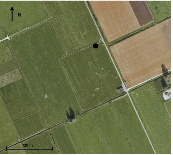
meteorological observatory, where continuous measurements of air and soil temperature, air humidity, radiation, wind direction and wind speed are available. The measurement site is located west of Wageningen in The Netherlands (51° 58' 18'' N; 5° 38' 30'' E) on a heavy clay soil with a temperate humid perennial ryegrass pasture (Lolium perenne) (Van Hove, 1989). Figure 4 shows an aerial overview of the meteorological observatory and its surroundings. The black dot represents the location of the ammonia gradient set-up. There is no application of manure at the site and grass is cut on average 3-4 times a year. The average elevation of the measurement site is 6.80m above mean sea level. (Webpage of observatory: http://www.maq.wur.nl).

Figure 4. Aerial view of the micrometeorological site 'Haarweg' in Wageningen, The Netherlands. (courtesy: Google Earth)

3.2

Instrumentation

3.2.1

Meteorological instrumentation

The micrometeorological weather station at the Haarweg in Wageningen is a Special Agro-Meteorological Station. Appendix A gives an overview of the standard (micro)meteorological variables that are measured at this observatory. Besides these standard meteorological variables, measurements of horizontal wind speed (U), wind direction, friction velocity (u*) and sensible heat flux (H) are

provided by a CSAT3 3-D sonic anemometer (Campbell Scientific) mounted at 3.5 m.

Meteorological variables are logged with a frequency of once every 10 minutes. The micrometeorological flux measurements, however, are averaged over a 30-minute time period. Since these data are required for the eventual ammonia flux calculations, all measurements are converted to 30-minute averages.

3.2.2

Ammonia instrumentation

The NH3-concentration profiles (needed in Eq. 14) are measured using the new GRadient Ammonia –

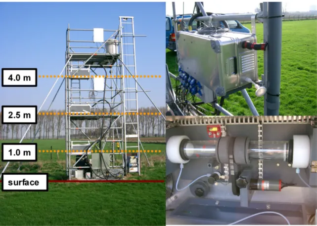
High Accuracy – Monitor (GRAHAM), a more advanced version of the AMANDA (a continuous rotating wet denuder analyzer; Wyers et al., 1993; Wichink Kruit et al., 2007). The GRAHAM (shown in Figure 5) is an instrument that measures the NH3-concentration at 1 m, 2.5 m (2.0 m from 30 May

2005 onwards) and 4 m height with a frequency of once every 10 minutes. The GRAHAM is well suited for micrometeorological measurements because of its low detection limit, high precision and accuracy and high time resolution. The measurement principle of the GRAHAM denuder is basically the same as the existing AMANDA denuder as described by Wyers et al. (1993, 1998).

Figure 5. GRAHAM measurement system (left), close up of one of the three denuder boxes (upper right) and close up of an annular denuder inside the box (lower right).

The GRAHAM uses horizontally-positioned rotating annular denuder tubes. A denuder tube consists of two concentric glass tubes of 30 cm in length and up to 50 mm in diameter. The walls of the annular denuder are coated with a slightly acidic absorption fluid (3.6 mM NaHSO4). Air is pumped through

the space between the two glass tubes at a rate of approximately 23 l min-1. Any gaseous ammonia present in the air diffuses to the walls of the denuder, where it is captured by the absorption fluid. Ammonium aerosol (NH4+) passes through the denuder almost unimpeded (only 1-2% absorption) as

the diffusion rate of aerosols is much smaller than that of the gaseous NH3.

The absorption fluid is continuously pumped through the denuders at a rate of 1 ml min-1 and flows in opposite direction to the air flow. The absorption fluid containing the dissolved NH3 (as NH4+) is now

analyzed by a common detector. Once in the detector, the absorption fluid containing NH4+ is mixed

with a solution of 0.5 M NaOH, so that molecular ammonia is formed again. This molecular ammonia diffuses through a semi-permeable PTFE membrane and is dissolved in de-ionized water present on the other side of the membrane. At pH lower than 7, it is mostly present in the form of NH4+ and the NH4+

concentration in this water flow is determined by conductivity. The analyzer is calibrated with aqueous standards of typically 0, 50 and 500 µg l-1 NH4+. The detection limit of NH3 in air is approximately

0.02 µg m-3.

Several modifications have been carried out with respect to the AMANDA to improve the accuracy as well as the precision of the instrument. In the old AMANDA system flow rates were determined manually at service visits. In the current GRAHAM system continuous in-line airflow measurements are implemented, which is an obvious improvement with respect to the precision and accuracy. The

flow rates are determined by measurements of temperature and the pressure drop over a restriction. To minimize systematic errors the restrictions have been brought together in an aluminium body.

Second, two 3-channel syringe pumps (type Mechatronics) replaced the multi channel peristaltic pump allowing a well-defined sample flow from the denuders. With two coupled 10 ml syringes per denuder and a 1 ml min-1 sample flow a cycle time of ten minutes is obtained. During a cycle time the three samples are sequentially led through the detector allowing two minutes of flushing in between.

Third, the conical structure in the inlet is now also applied on the outlet of the wet rotating denuder. This optimized aerosol conducting system prevents ammonium containing particles (aerosols) from impaction on wetted surfaces and from being a potential source of interfering ammonium.

Average concentration values for all three denuders were determined during a 10 minute cycle. The 3 denuders were sampled sequentially with a stabilizing time of 2 minutes and an averaging time of 1 minute. After this cycle of 9 minutes, the detector is flushed for 1 minute and a new cycle starts. The tube length for transporting the solution to the detector is equal for all three heights to ensure that the concentrations measured in the analyzer refer to identical air sampling periods.

A vertical PVC pipe of diameter 0.1 m was attached to the three denuders to be able to mutually compare the three denuders in the field. A high volume of ambient air is blown through the pipe (about 200 m3 hr-1) to ensure that the concentration at all three denuder heights is the same during comparison. Each denuder samples the same air from this PVC pipe and should consequently measure the same concentration. Observed differences between the individual denuders can be considered as systematic differences. With this vertical PVC pipe, we are able to correct for the systematic differences between the denuders under field conditions. The procedure for systematic error correction is described in the following chapter.

4

Error analysis

4.1

Systematic and random errors in the concentration

4.1.1

Laboratory comparison

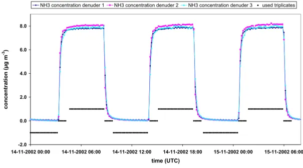
Data on the performance of the earlier version of this instrument (AMANDA) were reported by Wyers et al. (1993, 1998) and Mennen et al. (1996). Wyers et al. (1993) positioned three instruments in the field at the same height and averaged the measurements every 30 min. They corrected the obtained concentrations for systematic differences, and reported the between-instrument standard deviation based upon 22 simultaneous triplicates to be 2.6% relative over the entire time spanned by the concentrations. The correction method and the concentrations themselves were not reported. The current GRAHAM system was tested in a similar way. The three instruments were placed on a lab bench. They were simultaneously fed with the same sample, which was alternately clean air and 8 μg m-3 NH3, each period lasting about 5 hours on 14 and 15 November 2002 (see Figure 6). Readouts were

obtained every 10 minutes. The used triplicates are indicated with black dots in Figure 6 (1 = high concentration (about 8 μg m-3); 0 = transition period (between 0 and 8 μg m-3); -1 = low concentration (about 0 μg m-3_)).

NH3 concentration per denuder in time

-2.0 0.0 2.0 4.0 6.0 8.0 14-11-2002 00:00 14-11-2002 06:00 14-11-2002 12:00 14-11-2002 18:00 15-11-2002 00:00 15-11-2002 06:00 time (UTC) con cen trati o n (µg m -3)

NH3 concentration denuder 1 NH3 concentration denuder 2 NH3 concentration denuder 3 used triplicates

Figure 6. Laboratory concentration measurements for precision determination. The black diamonds represent the different situations during the concentration comparison test (1 = high concentration (about 8 μg m-3); 0 = transition period (between 0 and 8 μg m-3); -1 = low concentration (about 0 μg m-3).

If we assume that the average of the three concentrations in Figure 6 is the 'real' concentration, we can distinguish two types of systematic errors. The first type is the difference in delay times between the

three individual denuders. Figure 7 shows the absolute difference between the individual denuders and the average of the three denuders (i.e. the 'real' concentration) versus the change of the average concentration in time. An increase in concentration in time will lead to a higher increase for denuder 2 than the average increase in concentration, i.e. denuder 2 is 'too fast'. Denuder 3 gives a lower increase than the average increase in concentration and can therefore be considered as 'too slow'.

absolute error in the concentration per denuder vs. average NH3 concentration

y = -10.831x - 0.050 R2 _{= 0.047} y = 96.497x + 0.059 R2 _{= 0.775} y = -102.265x - 0.009 R2 _{= 0.816} -1 -0.8 -0.6 -0.4 -0.2 0 0.2 0.4 0.6 0.8 1 -0.01 -0.005 0 0.005 0.01

NH3 concentration change in time (µg m-3 s-1)

abso lu te erro r i n t h e con cen trat ion p er de nu de r (µ g m -3)

absolute difference between denuder 1 and average before correction absolute difference between denuder 2 and average before correction absolute difference between denuder 3 and average before correction Lineair (absolute difference between denuder 1 and average before correction)

Lineair (absolute difference between denuder 2 and average before correction)

Lineair (absolute difference between denuder 3 and average before correction)

Figure 7. The absolute difference between each denuder and the average concentration versus the concentration change in time (µg m-3 _s-1₎

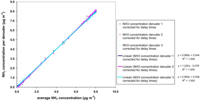
The second type of systematic error that was corrected is the regression of the measured concentrations per denuder (slope and offset) relative to the average concentration (Figure 8).

NH3 concentration per denuder vs. average NH3 concentration y = 0.989x + 0.044 R2 _{= 1.000} y = 1.020x - 0.078 R2 _{= 1.000} y = 0.993x + 0.026 R2 _{= 1.000} 0.0 1.0 2.0 3.0 4.0 5.0 6.0 7.0 8.0 9.0 0.0 2.0 4.0 6.0 8.0 10.0 average NH3 concentration (µg m-3) NH 3 con cen trat io n p er den u d er (µg m -3) NH3 concentration denuder 1 corrected for delay times NH3 concentration denuder 2 corrected for delay times NH3 concentration denuder 3 corrected for delay times

Lineair (NH3 concentration denuder 1 corrected for delay times)

Lineair (NH3 concentration denuder 2 corrected for delay times)

Lineair (NH3 concentration denuder 3 corrected for delay times)

Figure 8. Linear regression through the measured concentrations per denuder relative to the average concentration after correction for the different delay times.

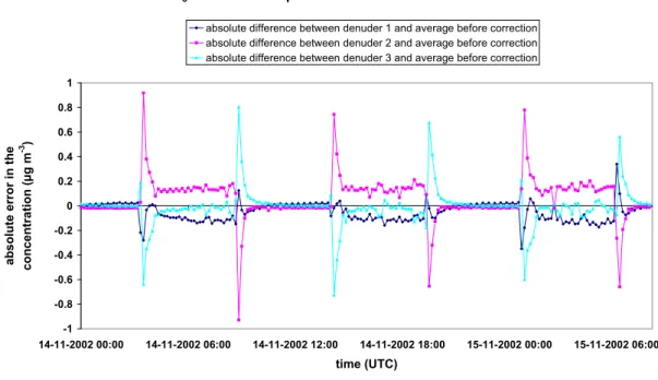
The figures below show the absolute difference between the measured concentrations per denuder and the average concentration before (Figure 9) and after (Figure 10) systematic error correction. The systematic error correction for the differences in delay times reduces the large peaks just after concentration change, while the systematic error correction for the linear regression reduces the differences between the individual denuders and the average.

The resulting absolute difference (between the measured concentration per denuder and the average concentration) after systematic error correction represents the random error (Figure 10). The figure shows that the random error is a little bit higher (and variable) in periods of quickly changing concentrations (transition periods), while it is rather low (and constant) in stationary conditions (around 0 and 8 µg m-3).

NH3 concentration per denuder in time before correction -1 -0.8 -0.6 -0.4 -0.2 0 0.2 0.4 0.6 0.8 1 14-11-2002 00:00 14-11-2002 06:00 14-11-2002 12:00 14-11-2002 18:00 15-11-2002 00:00 15-11-2002 06:00 time (UTC) ab so lu te er ror in th e con cen trat io n ( µ g m -3 )

absolute difference between denuder 1 and average before correction absolute difference between denuder 2 and average before correction absolute difference between denuder 3 and average before correction

Figure 9. Absolute difference between the measured concentrations per denuder and the average concentration before systematic error correction.

NH3 concentration per denuder in time after correction

-1 -0.8 -0.6 -0.4 -0.2 0 0.2 0.4 0.6 0.8 1 14-11-2002 00:00 14-11-2002 06:00 14-11-2002 12:00 14-11-2002 18:00 15-11-2002 00:00 15-11-2002 06:00 time (UTC) ab solute er ror in the co ncen tra tio n ( µ g m -3 )

absolute difference between denuder 1 and average after correction for delay times and slope and offset absolute difference between denuder 2 and average after correction for delay times and slope and offset absolute difference between denuder 3 and average after correction for delay times and slope and offset

Figure 10. Absolute difference between the measured concentrations per denuder and the average concentration after systematic error correction.

In order to be able to compare the performance of the GRAHAM with the performance of AMANDA, every three subsequent results of each denuder were averaged in order to obtain one triplicate every 30 min. The results of the error analysis in the concentration measurements corrected for systematic errors are shown in Table 2. The table shows the random errors for two different averaging times, e.g. 10 and 30 minutes. We also distinguished three different regimes, e.g. 0 µg m-3, between 0 and 8 µg m-3, and 8 µg m-3_.

Table 2. Random errors in the concentration measurements corrected for systematic errors for two averaging times (10 and 30 minutes) and three periods (0 µg m-3, 0-8 µg m-3 and 8 µg m-3)

10-minute average 30-minute average

absolute random error Relative random error Absolute random error Relative random error average deviation of the mean

concentration at 0 µg m-3

0.012 µg m-3 - 0.012 µg m-3 -

number of triplicates 48 48 16 16

average deviation of the mean concentration between 0 and 8 µg m-3

0.080 µg m-3 _{2% 0.058 µg m}-3 _1.45%

number of triplicates 36 36 12 12

average deviation of the mean concentration at 8 µg m-3

0.027 µg m-3 0.34% 0.018 µg m-3 0.23%

number of triplicates 75 75 24 24

The random error in the 10-minute average data in this laboratory test is 0.027 µg m-3 at 8 µg m-3, which corresponds to a relative random error of about 0.34%. The random error is even smaller at 0 µg m-3 (0.012 µg m-3), but much higher in the transition periods, 0.080 µg m-3. The relative random error in the transition periods (assuming an average concentration of 4 μg m-3) is about 2% and can mainly be ascribed to the differences in delay times between the individual denuders. The random error in the 30-minute average data is 0.018 µg m-3 at 8 µg m-3, which corresponds to a relative error of about 0.23%. The random error at 0 µg m-3 is 0.012 µg m-3 again and the random error in the transition period is 0.058 µg m-3 _{(or about 1.45%).}

4.1.2

Field comparison

During a field comparison 'campaign' of 10 days in June 2004, a precision test was done with the attached PVC pipe (described in Chapter 3.2.2). Concentrations roughly varied between 4 and 50 μg m

-3 _{during this period and all three denuders showed a similar pattern. To estimate random errors in the}

concentration measurements, data are corrected for systematic errors following the procedure described

before. We only considered concentration measurements between 0 and 20 µg m-3 to have a

homogeneous distribution of concentrations and to be sure that possible saturation effects were excluded. Before the systematic error correction, the average difference between each denuder and the average of the three denuders was 0.05 µg m-3 at an average concentration of 8.77 µg m-3, so about 0.6 %. After systematic error correction, this difference is reduced to zero by definition.

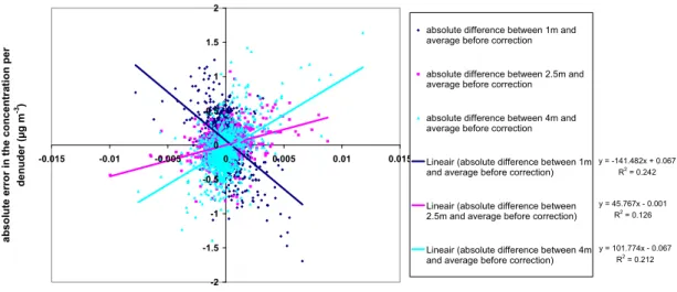
Figure 11 shows the absolute difference between the individual denuders and the average of the three denuders versus the concentration change in time. This yields a systematic error correction due to differences in delay times between the individual denuders. Figure 12 shows the regression of the

measured concentrations per denuder (corrected for differences in delay times) relative to the average concentration. This is the second systematic error correction to correct for the slope and the offset.

absolute error in the concentration per denuder vs. average NH3 concentration

y = -141.482x + 0.067 R2 _{= 0.242} y = 45.767x - 0.001 R2 _{= 0.126} y = 101.774x - 0.067 R2 = 0.212 -2 -1.5 -1 -0.5 0 0.5 1 1.5 2 -0.015 -0.01 -0.005 0 0.005 0.01 0.015

NH3 concentration change in time (µg m-3 s-1)

ab sol u te e rro r i n th e co n cen tra tio n p e r de nu de r ( µ g m -3)

absolute difference between 1m and average before correction

absolute difference between 2.5m and average before correction

absolute difference between 4m and average before correction

Lineair (absolute difference between 1m and average before correction)

Lineair (absolute difference between 2.5m and average before correction)

Lineair (absolute difference between 4m and average before correction)

Figure 11. Absolute difference between each denuder and the average concentration versus the concentration change in time (µg m-3 _s-1₎

NH3 concentration per denuder vs. average NH3 concentration

y = 0.999x + 0.013 R2 = 0.993 y = 1.006x - 0.054 R2 = 0.998 y = 0.995x + 0.041 R2 = 0.993 0.0 5.0 10.0 15.0 20.0 25.0 0.0 5.0 10.0 15.0 20.0 25.0 average NH3 concentration (µg m-3) NH 3 c on ce nt ra ti on p er de nu de r (µ g m -3) NH3 concentration at 1m corrected for delay times

NH3 concentration at 2.5m corrected for delay times

NH3 concentration at 4m corrected for delay times

Lineair (NH3 concentration at 1m corrected for delay times) Lineair (NH3 concentration at 2.5m corrected for delay times) Lineair (NH3 concentration at 4m corrected for delay times)

Figure 12. Linear regression through the measured concentrations per denuder relative to the average concentration after correction for the different delay times.

To compare the results from this field comparison with the results in the laboratory, the absolute between-instrument differences are calculated. Figure 13 shows the random error as a function of the average NH3 concentration. The random error in the measurements increases with an increasing NH3

concentration. This means that the random error for an average concentration of about 8 µg m-3 is 0.16 µg m-3.

absolute error in the concentration per denuder vs. average NH3 concentration

y = 0.0235x R2 _{= 0.1502} y = 0.0121x R2 = 0.1725 y = 0.0212x R2 _{= 0.1162} 0 0.2 0.4 0.6 0.8 1 1.2 1.4 0 5 10 15 20 average NH3 concentration (µg m-3) ab so lu te er ror in t h e co nc en trat io n pe r d en ude r (µ g m -3)

absolute difference between 1m and average after correction for delay times and slope and offset

absolute difference between 2.5m and average after correction for delay times and slope and offset

absolute difference between 4m and average after correction for delay times and slope and offset

Lineair (absolute difference between 1m and average after correction for delay times and slope and offset)

Lineair (absolute difference between 2.5m and average after correction for delay times and slope and offset)

Lineair (absolute difference between 4m and average after correction for delay times and slope and offset)

Figure 13. Random error as a function of the average NH3 concentration for the three measurement

heights.

We conclude that the precision of the instrument in the field (1.9%) is comparable to the precision of the instrument in the laboratory in transition periods (about 2%). Although the average concentration changes in the field are generally smaller than the concentration changes (8 μg m-3) in the transition periods in the laboratory, weather influences such as substantial temperature and humidity changes are likely to affect the precision. In the presented results, a random error of 1.9% (based on the field comparison) is applied on the concentration measurements. The systematic error of 0.6% in the concentration measurements was corrected and is not present in the flux calculation. In Chapter 4.3, we will investigate how large the effect of this systematic error correction would be on our flux calculation (in the hypothetical case that we would not correct our concentration measurements for the known systematic errors).

4.2

Random error in the flux

For quantities that are a function of several parameters, a combined random error is calculated. The relative random error in our flux calculation,

F

_χ

=

−

u

_∗

χ

_∗ (Equation 6), is given as:

2 * * 2 χ χ χ δχ u u δ F F δ ⎟ ⎟ ⎠ ⎞ ⎜ ⎜ ⎝ ⎛ + ⎟ ⎟ ⎠ ⎞ ⎜ ⎜ ⎝ ⎛ = ∗ ∗ ₍₁₆₎

The random error in the friction velocity (δu*) is calculated with the ECpack software developed by

Wageningen University (Van Dijk et al., 2004; freely available at http://www.maq.wur.nl). Figure 14 shows that the relative random error in the friction velocity is about 4-5%. The relative random error in u* is rather constant during the day, whereas relative random errors higher than 5% mainly occur during

daily course of the relative random error in u* 0 2 4 6 8 10 0 6 12 18 24 time (UTC) re lative random e rror in u * (%)

Figure 14. Daily cycle of relative random error in u* for the entire data set.

The random error in χ* is more difficult to determine. We start with rewriting Equation 10b into:

⎟ ⎠ ⎞ ⎜ ⎝ ⎛ + ⎟ ⎠ ⎞ ⎜ ⎝ ⎛ − ⎟⎟ ⎠ ⎞ ⎜⎜ ⎝ ⎛ − = ∗ L z Ψ L z Ψ z z ln ) z ( χ ) z ( χ k χ 1 χ 2 χ 1 2 1 2 ₍₁₇₎

The relative random error in χ* is described as:

[

]

2 2 1 2 1 2 ) Ψ , z ( f ) Ψ , z ( f δ ) z ( χ ) z ( χ ) z ( χ ) z ( χ δ χ δχ ⎟ ⎟ ⎠ ⎞ ⎜ ⎜ ⎝ ⎛ + ⎟ ⎟ ⎠ ⎞ ⎜ ⎜ ⎝ ⎛ − − = ∗ ∗ ₍₁₈₎

where: δ

[

χ(z₂)−χ(z₁)

]

=

(

δχ(z₂)

) (

2+ δχ(z₁)

)

2 represents the random error in the concentration difference (the numerator in Equation 17, shown as error bars in Figure 15 together with the daily cycle of the concentration difference), and represents the random error in the stability corrected height (the denominator in Equation 17; abbreviated as f(z,Ψ) in Equation 18). Assuming that the errors in the heights of the measurements (z1 and z2) are negligible, the error in the stability corrected height

in Equation 18 is only determined by errors in the stability corrections. However, the errors in the stability corrections are difficult to determine as they are complex functions of the Obukhov length. In this study we assume a relative random error in the stability correction functions of 5% (Nieuwstadt, 1978; Holtslag and Van Ulden, 1983).

) Ψ , z ( f δ

Figure 16 shows the daily cycle of the relative random error in χ* (Equation 18).

daily course of the concentration difference -0.5 0 0.5 1 1.5 2 2.5 3 0 6 12 18 24 time (UTC) conc entra tion differe nce (µ g m -3)

Figure 15. Daily cycle of the concentration difference for the entire data set.

daily course of the relative random error in X*

0 20 40 60 80 100 120 140 160 0 6 12 18 24 time (UTC) rela tive ra ndom error in X * (%)

Figure 16. Average daily cycle of the relative random error in χ* for the entire data set. (peak value is

255%)

The random error in the flux estimate is calculated by multiplying the relative error in the flux by the absolute value of the flux, according to:

2 * * 2 χ χ F δ_uu δχ_χ F δ _⎟⎟ ⎠ ⎞ ⎜ ⎜ ⎝ ⎛ + ⎟ ⎟ ⎠ ⎞ ⎜ ⎜ ⎝ ⎛ ⋅ = ∗ ∗ ₍₁₉₎

Figure 17 shows the random error in the flux estimate for the entire data set. The random error in the flux estimate is largest (about 0.06 µg m-2 s-1) in the early morning and during daytime mainly due to

small concentration differences, whereas it is relatively small (about 0.01 µg m-2 s-1) during night time, when concentration differences are relatively large. On average the random error in the flux estimate is about 0.03 µg m-2 s-1.

daily course of the absolute random error in the flux estimate

0 0.02 0.04 0.06 0.08 0 6 12 18 24 time (UTC) absolute random er ror in flux e stimate (µg m -2 s -1) Figure 17. The daily cycle of random error in the flux estimate for the entire data set.

If we look at the relative random error in the flux measurement (Figure 18), i.e. the (absolute) random error in the flux divided by the flux, we see that the relative random error is rather small (in the order of about 20%) during night time, when the gradient is well defined, and becomes very large (over 100%) during daytime, when the concentration differences and consequently the fluxes approach zero.

daily course of the relative random error in the flux estimate

0 20 40 60 80 100 120 140 160 0 6 12 18 24 time (UTC) re lativ e random e rror in flux es timate (%)

Figure 18. The daily cycle of relative random error in the flux estimate for the entire data set. (peak value is 255%)

Table 3 gives an overview of the observed ranges for the daily cycle of the different parameters in the flux calculation. It also shows the ranges for the absolute and relative random error in the different parameters in the flux calculation.

Table 3. Overview of ranges for the absolute and relative random error in the flux calculation parameters.

parameter mean Absolute random error Relative random error

χ 10.0 μg m-3 (7.3 - 12.7) 0.19 μg m-3 (0.14 - 0.24) 1.9%

u* 0.18 m s-1 (0.13 - 0.25) 0.008 m s-1 (0.006 - 0.011) 5% (4 - 7)

χ(z2) - χ(z1) 1.01 μg m-3 (0.08 - 2.24) 0.27 μg m-3 (0.20 - 0.34) 52% (15 - 255)

χ* 0.41 μg m-3 (0.08 - 1.53) 0.16 μg m-3 (0.05 - 0.39) 52% (15 - 255)

Fχ -0.07 μg m-2 s-1 (-0.02 - -0.24) 0.03 μg m-2 s-1 (0.01 - 0.07) 52% (15 - 255)

The relative random error in the flux calculation varies between 15% during night time and 255% during daytime. The average relative random error in the flux estimate is about 52% (the median value is 31%). Note that these large relative random errors are mainly caused by the (relatively small) random errors in the concentration measurements in combination with the small concentration differences.

4.3

Effects of systematic errors in concentration measurements on

the flux

To investigate the effect of the systematic errors in the concentration measurements on the flux estimates (e.g. to see if systematic errors can lead to a different sign for the flux), we compared the flux measurements without correction for systematic errors with the flux measurements with corrections for systematic errors (like described in the previous Chapters). Figure 19 shows the daily cycle of the calculated systematic error in the flux estimate (flux without systematic error correction - flux with systematic error correction). The systematic error in the flux estimate is about 2 times smaller than the random error in the flux estimate (solid line compared to the dashed line). The systematic error in the flux estimate is largest in the morning (i.e. about 0.03 µg m-2 s-1) mainly due to large concentration changes in time, while it is relatively small during night time (i.e. about 0.005 µg m-2 _s-1_{), when there}

might be large concentration changes, but there is minimum exchange.

Figure 20 shows the average daily cycle of the 'best' flux estimate (black solid line) with the random errors (error bars). The flux calculated without the systematic error corrections (black dashed line) does not significantly affect the pattern of the daily cycle of the flux and only seem to influence the size of the mean (annual) flux.

Several short comparison tests (of about 1 day) in 2004 indicate that the systematic error corrections obtained from the 10-day comparison period are representative for the whole period, although the slopes and the offsets might sometimes change sign (opposite systematic error correction) or are larger (larger systematic error correction) than the slopes and offsets used in this study. Since these short comparison tests only concern few measurements and a very limited concentration range, they are considered to be highly uncertain and inadequate for intermediate data correction. Therefore, we decided to use the systematic error corrections from the 10-day comparison period to correct all our data.

daily course of the absolute systematic and random error in the flux estimate 0 0.02 0.04 0.06 0.08 0 6 12 18 24 time (UTC) a bsolute e rror in flux estima te (µg m -2 s -1)

absolute systematic error in the flux estimate absolute random error in the flux estimate

Figure 19. The daily cycle of the absolute systematic (solid line) and random (dashed line) error in the flux estimate for the entire data set.

Effect of systematic error correction on flux estimate

-0.30 -0.20 -0.10 0.00 0.10 0 6 12 18 24 time (UTC) flux e stimate (µg m -2 s -1) flux estimate without systematic error correction best flux estimate

Figure 20. Average daily cycle of the flux estimate (solid black line) and the random errors (error bars) for the entire data set. The dashed line represents the flux estimate without systematic error corrections to show the sensitivity for systematic error corrections in the flux estimate.

4.4

Summary uncertainties and concluding remarks

4.4.1

Errors in the concentration

In a laboratory comparison test, a random error of 0.027 µg m-3 at 8 µg m-3 is found in the 10-minute average data after systematic error correction, which corresponds to a random error of about 0.34%. The random error at 0 µg m-3 is even smaller (i.e. 0.012 µg m-3). On the other hand, the random error in the transition periods (between 0 and 8 and vice versa) is much higher, i.e. 0.080 µg m-3, which corresponds to a random error of about 2% (assuming an average concentration of 4 μg m-3).

In a field comparison test of 10 consecutive days, we obtained that the average systematic error in the concentration between the three denuders is about 0.6% at an average concentration of 8.7 µg m-3. After systematic error correction, this systematic difference reduced to zero by definition. The random error in the concentration that remained after this systematic error correction was 0.17 µg m-3 at an average concentration of 8.7 µg m-3, which corresponds to a random error of 1.9%.

So, the random error in a concentration measurement under field conditions (1.9%) is much larger than the random error in a concentration measurement under stable laboratory conditions (0.34%). This difference is mainly caused by a continuously changing concentration in the field, while in the laboratory the concentration was kept constant until it stabilized. The random error in the transition periods in the laboratory comparison of 2%, however, compares well with the random error found in the field comparison.

4.4.2

Errors in the flux

After correcting our concentration measurements for systematic errors, the flux can be calculated as described in Chapter 2.2. However, the random errors in the concentration measurements (1.9%) propagate in the flux calculations and result in an average random error in the calculated fluxes of 52% (median value is 31%). Large differences are observed between the random error in the flux calculation during nighttime (15%) and during daytime (255%). The large random errors during daytime are mainly caused by small concentration differences in combination with the random errors in the concentrations at the different heights. During nighttime, these concentration differences are considerably larger and consequently, the random error in the flux calculation is smaller.

If we would not correct our concentration measurements for systematic errors, an average systematic

error in the flux calculation of 18% would be made. However, because we assume that the systematic

error corrections are justified and correct, there is no systematic error present in our final flux calculation. However, if the systematic error correction in the concentration measurements is applied unjustified, the error that we make in the flux calculation as a consequence of the systematic error correction is relatively small (18%) compared to the random error in the flux calculation (52%) on an hourly basis.