Comparison of global passenger transport models and available literature | RIVM

(1)

Comparison of global passenger transport models and available literature

RMH Breugem, DP van Vuuren, B van Wee

This investigation has been performed by order and for RIVM MAP-SOR within the framework of project 461502, IMAGE Ontwikkeling en Beheer.

(2)

Abstract

Over the last decade transport has been strongest growing sector in terms of worldwide energy demand. As a result, proper modelling of transport has become more important in models describing global climate change. RIVM has developed the energy model TIMER as part of the global integrated assessment model, IMAGE (Integrated Model to Assess the Global Environment) to study long-term energy scenarios, related environmental problems and available options for mitigation (up to 2100). In the research project described, the aim was to find a modelling approach and identify determinants of transport energy demand to improve the projections of TIMER, focusing on passenger transport. Global transport models were compared by means of a literature study.

The literature that could be reviewed for this project focused mainly on passenger transport in OECD countries. In addition, four global transport models were studied – i.e. two models from the World Energy Council, one from the International Energy Agency, and a model described by Schafer and Victor. On the basis of this review, it became clear that the best improvements could be achieved in transport modelling in the context of TIMER by adopting an updated version of the transport model by Schafer and Victor. Such a model would take into account the determinants, technology, spatial organisation (population density), prices and possible demographic factors other than population size (e.g. age).

(3)

Samenvatting

In de afgelopen jaren is wereldwijd het energieverbruik in de transport sector zeer sterk gegroeid. Het goed modelleren van transport in “integrated assessment” modellen is daarom steeds belangrijker. Als onderdeel van het mondiaal milieumodel IMAGE (Integrated Model to Assess the Global Environment) heeft het RIVM het TIMER model ontwikkeld om lange termijn energie scenarios en gerelateerde milieuproblemen te verkennen. De huidige

beschrijving van transport in het TIMER model is tamelijk geaggregeerd. In deze studie wordt een overzicht gegeven van de kennis in literatuur over de determinanten van de vraag naar energie van transport in het algemeen en van personenvervoer in het bijzonder.

Bovendien is een overzicht gemaakt van enkele bestaande modellen die mondiaal transport beschrijven. Op basis van dit overzicht worden suggesties gedaan hoe de modellering van transport in TIMER eventueel kan worden verbeterd.

De literatuur die binnen het tijdstip van dit onderzoek beschikbaar kon worden gemaakt is met name gericht op OECD landen en personenautogebruik. In deze literatuur komen

verschillende determinanten van transport activiteit en gerelateerd energiegebruik naar voren. De belangrijkste determinanten (met geoperationaliseerde variabelen) zijn economische ontwikkeling (bruto nationaal produkt), ruimtelijke indeling (urbane bevolkingsdichtheid), prijzen (brandstofprijzen, ticket prijzen), demografische factoren (bevolkingsomvang, leeftijd, geslacht) en technologische ontwikkeling (modale energie intensiteiten).

In de beschikbare literatuur kon van vier transport modellen een goede beschrijving gevonden worden. De twee modellen van de World Energy Council uit 1995 en 1998 zijn tamelijk simpele modellen waarin geen terugkoppelingen in de modelstructuur zijn opgenomen. In het 1995 model zijn de verwachtingen ten aanzien van economische, demografische en

technologische ontwikkeling en transport activiteit exogeen in drie verschillende scenarios opgenomen. Het 1998 model heeft naar alle waarschijnlijkheid een gelijke modelstructuur als het 1995 model.

De structuur van het transport model van de International Energy Agency is gecompliceerder en incorporeert een personenauto stock-turnover model. Ook vormen regionale

brandstofprijzen een belangrijke determinant.

Het transport model van Schafer en Victor richt zich alleen op personenvervoer. In dit model zijn de twee theorema van Zahavi opgenomen die poneren dat de mens een vast deel van zijn inkomen en een constante hoeveelheid tijd aan vervoer besteed. Ook gaat het model ervan uit dat bepaalde transport infrastructuren voor lange tijd de vervoerswijze in de toekomst

bepalen. Daarnaast is ruimtelijke ontwikkeling expliciet opgenomen als determinant van de keuze voor een bepaald vervoersmiddel.

Op basis van de literatuurstudie en persoonlijke communicatie met Schafer lijkt de aanpak van Schafer and Victor in combinatie met een model om het energiegebruik van

vrachtvervoer te beschrijven een goede methode voor de beschrijving van transport energiegebruik in TIMER.

(6)

Summary

Transport has developed into the strongest growing sector in terms of worldwide energy demand. As a result, proper modelling of transport is becoming more important in models describing global climate change. RIVM has developed the energy model TIMER as part of the global integrated assessment model, IMAGE (Integrated Model to Assess the Global Environment) to study long-term energy scenarios, related environmental problems and available options for mitigation (up to 2100). The description of the transport sector in this model is fairly aggregated. Within this research project, suggestions to improve the current formulation of transport in TIMER, have been made, focusing on passenger transport. These suggestions are based on an overview of transport-related literature (focusing mainly on OECD countries and car transport) and on the comparison and evaluation of global transport models.

Various determinants of transport activity and related energy consumption are identified in the existing literature. The most important determinants (with operationalised variables) are economic development (GDP), spatial organisation (urban population density), prices (fuel,ticket), demographic factors (population size, age, gender) and technological development (modal energy intensities, fuel economies).

Fairly detailed descriptions could be found of four global transport models in the available literature. Two of these, from the World Energy Council (1995, 1998), are relatively simple and do not contain any feedback relationships. In the 1995 model the expectations with respect to economic, demographic and technological development and transport activity were taken up exogenously in three different scenarios. The 1998 model probably has a similar model structure but does not adopt any scenarios.

The structure of the model of the International Energy Agency is more complicated and incorporates a private-car stock turnover model. Also regional fuel prices play an important role.

The transport model of Schafer and Victor only addresses passenger transport. In this model, two theorems of Zahavi state that on average people spend a fixed amount of their income and a constant amount of time on travelling. The Schafer and Victor model also assumes that certain transport infrastructures determine the use of specific modes of transport for the long term. Furthermore, spatial organisation has explicitly been taken up as a determinant of the choice for a certain transport mode.

On the basis of the literature study and personal communication with Schafer, we decided that the Schafer and Victor approach could provide the best opportunities to improve the description of future transport energy use in TIMER. The current model, however, needs to be extendend with a model describing freight transport energy use.

(7)

1. Introduction

In the 1990 – 1995 period, transport was the fastest growing sector in terms of its energy demand. Between 1971 and 1990, world transport energy demand grew by 2.8% per year, which is slightly faster than the growth rate of total energy demand (2.5%). Since 1990, the growth of transport energy demand declined to 1.7% per year – but the growth rate of total energy demand dropped even further to 0.7%. The share of transport in total world energy demand is around 20-25%. For the future it is expected that transport will continue to increase its share in the global energy demand. This is likely going to present serious problems with regard to congestion, safety and emission of environmental pollutants like greenhouse gasses (GHG). Proper modelling of transport becomes thus more and more important in models describing global climate change.

0 30 60 90 120 1970 1975 1980 1985 1990 1995 E J/ yea r Industry Sector Transport Sector Buildings Agriculture

Figure 1-1 Global energy consumption from 1971 to 1995 (Based on IEA, 1998)

As part of the global climate change model IMAGE, the TIMER energy model was developed by the RIVM (Netherlands Institute for Public Health and the Environment) to study long-term energy scenarios, related environmental problems and available options for mitigation (up to 2100). This model is gradually being extended to include more detailed information on the physical realities behind the different scenarios1. Currently, the description of transport energy demand in TIMER is rather simple, just like other energy demand sectors in the model. In this research project, an attempt would be made to find a modelling approach and identify determinants of transport energy demand to improve the projections of TIMER, focusing on passenger transport.

Transport activity is generally divided between passenger transport and freight transport. For this study, we chose to address passenger transport only. In 1995, passenger transport

contributed to 57% of total transport energy consumption World Energy Council (1998). In Figure 1- presents the position of the system examined (global passenger transport energy consumption) within the total energy system. The division of global energy consumption over

(8)

the different sectors is taken from TIMER (year 1990). The modal split in 1990 is derived from Schafer (1998). The split between freight and passenger transport is based on passenger transport data from Schafer (1998) and total transport energy demand from TIMER.

Figure 1-2 System boundaries and share in energy consumption, 1990.

Chapter 2 outlines the methodology of this study. In fact, the study starts with a literature study to obtain insight into the relationships of transport activity and energy consumption with several determinants. The results of this literature search are presented in Chapter 32. Chapter 4 presents four largely independent global transport models and one model, partly derived from one of the previous four. In Chapter 5, the first four models are compared and evaluated. Next, in Chapter 6 a very brief overview is given of several energy demand scenarios of different models (mostly very aggregated models), in particular to give an indication of how the current TIMER performs in comparison with other global energy models. Chapter 7 discusses the models in relation to three important determinants. Finally, in Chapter 8, an idea is presented that could serve as a framework for the implementation of the identified improvements in TIMER.

2_{Please note that Chapter 3 is not intended to give a full summary of the reviewed articles and reports but that it}

identifies determinants of transport activity or energy consumption.

Cars

(52%) Buses(29%) (9.5%)Rail

Global freight transport energy use (40%) Global passenger transport energy consumption (60%)

Transport (24%)

Global energy consumption Commercial (8%) Residential (33%) Industry (32%) Other sectors (4%) Air (9.5%)

(9)

2. Methodology

One can identify five general steps in the development of a conceptual model to an

operational model. The first step comprises the development of a conceptual model. In the second step, the variables are identified that reflect the content of the determinants of the conceptual model. In the third step, the relationships between the variables are determined. In step 4, the values of the various parameters are determined (calibrated) on the basis of

historical data sets and in step 5, projections of autonomous (independent) variables are made to feed the model. Although the intention of this study is not to build a new transport energy model, but to review a set selected existing models, nevertheless these steps can more-or-less connected to our activities.

First, we will discuss some of the available transport literature to develop an idea of how the conceptual model of a good transport model should look like. Chapter 3 shows the results of this review of mainly car transport-related literature on OECD countries. Although it was not our intention to focus on car transport only, most of the available literature focussed on car transport. This can be explained by the large share of car transport in the modal split. We noticed that the literature addressing the complete overview of passenger transport was fairly limited. More literature was found on detailed topics like vehicle ownership or CO2 emissions

as a result of global transport. Chapter 3 focuses on identifying determinants of the three variables in Figure 2-1, which according to Schipper (1997) determine passenger transport energy consumption. “A” denotes total travel expressed as passenger kilometres, “S” denotes the modal split (relative participation of the various transport modes in total transport) and “I” is the specific modal energy intensity (the energy which a specific transport mode consumes per km).

Figure 2-1 Passenger transport energy consumption.

The modal energy intensity term itself is composed of several components based on Schipper, 1997):

Ii = Ei * Ci * Ui (1)

where E is technical efficiency, C vehicle characteristics, and U the inverse of capacity utilisation for each mode i. Ei * Ci is the energy use per vehicle kilometre and is called

vehicle fuel intensity. The technical efficiency is the energy required to propel a vehicle of a given set of characteristics a given distance, and is affected by the motor, drive train,

frictional terms (including drag) etc. For cars, characteristics could be represented by vehicle power (or gross weight) and technical efficiency by energy use per km per unit of power (or gross weight). People/vehicle or tonnes per vehicle could measure capacity utilisation U. In Chapter 4 an inventory of global transport models is made. These models are described and compared. In addition we have looked at whether the models include the determinants found in Chapter 3.

Total travel (A) x Modal share (S) x Modal energy intensity (I)

(10)

Next, attention is paid to strengths/weaknesses of these models. In particular attention is paid to the question, how, based on these models possible improvements can be implemented in TIMER.

The determinants that turned out to affect passenger mobility are tested for their applicability in the TIMER model. The constraints that limit applicability are the operationalbility of the determinants, data availability and the specific TIMER requirements (degree of detail, etc). The first constraint refers to the ability to identify one or more variables that are able to reflect the meaning of a determinant. An example is whether aviation fuel price is a good representation of the costs of flying. The second constraint is the data availability of the selected variable. Some modelling approaches can not be adopted since data availability is limited. The last constraint refers to requirements imposed by TIMER, like compatibility with the applied level of detail. Is it useful to describe/model transport energy consumption with a high level of detail while other sectors contributing (approximately) equally to total energy consumption (e.g. industry) are modelled with only moderate detail?

Figure 2-2 presents a graphical visualisation of the above-mentioned methodology.

Comparison and Evaluation of Existing Global Transportation

Models Identified Determinants Strengths/weaknesses Determinants Approach Selection Operationilisibility Available data TIMER requirements

Results of first two steps Constraints (third step)

Applicable variables

TIMER Literature

(11)

3. Identifying determinants of passenger mobility

energy demand

Breaking down energy use into different variables as presented in Chapter 2 can give us some grip, while searching for determinants affecting passenger mobility, as many literature

sources discuss developments and projections of the variables shown in Figure 2-1 or equation (1). An overview at the end of this chapter gives the topics emphasised in the literature reviewed in the chapter. Note that this chapter, unless otherwise clearly stated, only represents the content of the articles and the reports.

3.1 Schipper (1997)

In Schipper (1997) an indication is given of how the World Bank could use its policy influence, and lending and analytical capabilities, to contribute to mitigation of CO2

emissions in the transport sector. With examples of OECD countries, important relationships are illustrated, which are often difficult to identify in non-OECD countries due to lack of data and measurement problems. Schipper discusses among other things the theses important for the World Bank’s policy: involvement of local authorities, transportation policies of OECD countries, pricing strategies, urban planning, lending and the World Bank’s analytical capabilities.

The summary here will focus on the determinants of transport energy consumption. In Figure 2-1 and equation (1) it is shown which variables could be influenced to decrease transport energy demand and CO2 emissions. Some of these variables show interdependency. For

example, total travel, A, depends on speed, so a shift in the modal split, S, from car to air is associated with greater travel. Secondly, I determines the marginal fuel costs of using vehicles. Transportation variable costs decrease to the same extent as I decreases and, as a result, transport demand might increase.

The author argues that the variables mentioned are generally affected by income, prices, technology, policy and behaviour. The number of passenger kilometres A and modal split S are dependent on income and prices. Personal travel depends in part on the distance between work, home, leisure and services, all depending on the spatial organisation of these

destinations. In societies with lower incomes and little motorised travel, or in societies with higher incomes, where congestion or other factors make travel expensive or slow, facilities are close together or individual radii of action are small. Where travel is cheap or rapid, markets cover much wider areas, and so do people. All of these dimensions are expanded with higher incomes. Price strategies are also expected to induce technological advances. Higher variable costs will stimulate development of energy efficient vehicles.

The vehicle intensity (E * C) is affected by both technological development and vehicle characteristics. Old and heavy cars have higher vehicle intensities than new and lightweight vehicles. In the last years people tend to drive more comfortable and heavier cars, partly offsetting the improved motor efficiency. Closer examination of trends in OECD countries has confirmed this development. While the average tested fuel use per kilometre driven and per kilogram of new cars fell dramatically in all countries, the weight (and performance) of new cars increased in all countries, absorbing much of the effect of improved technology.

(12)

Worsening driving conditions also proved to have significant impact on the vehicle

efficiency. Both more high-speed vacation driving and driving in congested areas raised fuel use per km above what tests would predict. Actual fuel use per km fell dramatically in the U.S. and Canada but barely changed in Japan and most European countries.

The variable U3 turns vehicle intensities into modal intensities. Increasing income causes people to value luxury and comfort more, lowering the occupancy degree of the vehicle and increasing the vehicle intensity by buying larger and heavier cars, overall increasing the modal intensity.

Schipper (1997) also shows that geographical organisation has influence on mobility and travel behaviour. A comparative study between San Francisco and Stockholm proved significant differences in mobility and modal split due to the difference in urban forms and physical layout of cities. Stockholm residents travel only a quarter of the distance San Franciscans do, the large difference partly explained by the fact that, in general, the Swedish travel only half the distance Americans do. Still, according to Schipper (1997), it could be said that urban structure – represented by population density – affects travel.

The relationships as described above are graphically shown in Figure 3-1.

Total travel Modal split Vehicle fu el intensity

Income Prices Urban Form

Technology Vehicle

Characteristics

Figure 3-1 Relationship between equation variables and determinants as presented in Schipper (1997).

Table 3-1 represents a summary of a larger interaction matrix shown in Schipper (1997). It shows to what extent policies affect the variables in Figure 2-1.

3_{The vehicle occupancy U has been used in many U.S. cities as an important policy element. By reserving lanes}

(13)

Table 3-1 Interaction between policy and mobility, and modal share and intensity

Component/Option A (Mobility) S (Modal share) I (Intensity) (veh.

intensity,

characteristics, load factor)

Vehicle Fuel

Economy Technology

None except through rebound

Slightly encourages modes with lower running costs

All

Overall fuel taxation Slight restraint, elasticity low

Favours modes with low fuel intensities

Encourages improvements in all factors Kilometer pricing (including congestion pricing)

Significant restraint. Favours modes with small footprints per passenger (ie. Bus, train)

Little effect unless small vehicles selectively permitted

Alternative fuels: development, pricing

Little effect unless price of fuel forced up

Little unless “clean fuel” modes given priority

Little, unless clean fuel more efficient

Land-use planning Supposedly would reduce total mobility

Could increase transit share

Little

3.2 Blijenberg and Van Swigchem (1997)

This paper discusses, among other things, trends in transport activity, associated energy use and some driving forces. Attention is also given to ways achieve a sustainable passenger transport system. In this perspective, the zero-emission vehicle, land use and policy implications are discussed.

In this summary, these driving forces are briefly mentioned and the effect of technological development, and the theory of constant travel time budget, are more closely examined. According to Blijenberg and Van Swigchem (1997), the main driving forces of travel mileage (or mobility) are time and money. The increasing travel mileage must be due to faster

transport modes and/or longer travelling time. Many economic and statistical sources show that faster transport is the dominant factor.

Some authors claim that something like a Constant Travelling Time Budget exists, valid throughout history and for all cultures. This is supported by some historical data indicating an average travelling time per person per day of around one hour and 5 to 20 minutes. Others indicate that travelling time depends partly on the amount of time spent on other activities, especially on the number of working hours Kraan (1996). As the average number of working hours is diminishing somewhat, the time available for other activities – including transport – may increase. If, in such a situation a faster mode of transport is introduced, this will reduce the total travelling time in the short term. In the longer term spatial patterns will change, resulting in greater travel mileage and longer travelling time. The opposite may occur as well: increased congestion will result in more time being spent on travel in the short term, but in the long term, mileage will be reduced and thus travelling time will decrease again.

The effect of technological development on the fuel intensity of vehicles is partly offset by the induced mobility. If, for example, motor efficiency is improved, the use of that vehicle

(14)

becomes cheaper due to a decrease in fuel use and will thus probably be used more intensively, increasing mobility, with a consequent partial offset of the fuel-use reduction gained. This situation supports the theory of the Constant Travelling Money Budget, more elaborately described in Schafer and Victor (2000) and Schafer and Victor (1999). In the Netherlands, the share of total income spent on transport from 1950 to 1988 increased only slightly (from 5.0% to 7.2%), but total expenditure on transport rose substantially. More money was spent on travel, resulting in both greater mobility and upgrading of cars Blijenberg and Van Swigchem (1997).

3.3 Banister (1996)

In Banister (1996) the emphasis is placed on the relationship of urban form and the energy consumption of transportation. Results from research in several cities in the U.K. proved that physical factors do have a significant effect on energy consumption, particularly gross density, measured in persons per hectare. In order to obtain still better results, the author’s advice was to develop a more sophisticated measure.

Open space within metropolitan areas also emerged as a significant factor in this study. From the perspective of the local authorities, there needs to be a balance between making cities more compact to limit transport needs, and maintaining and increasing the amount of open space, since this affects the attractiveness of the city.

Other factors, physical and socio-economic, turned out to be significant in some, but not all, examined cities (e.g. size of urban area, household size and car ownership). Other

relationships were found to have a variable sign (e.g. employment).

Finally, the author concludes that no definitive set of factors has been produced to determine the links between urban structure and energy use in transport. There seems to be consistency in the physical factors, but the socio-economic factors are also important taken individually. Furthermore, he states that it is still extremely difficult to obtain consistent data sets, either within towns (linking transport data with census, employment and other data sets) or between towns (different types of travel surveys).

3.4 Dargay and Gately (2001)

In this paper, the authors present the results of a model projecting the growth of vehicle stock over the next two decades for 82 countries at different levels of economic development. This paper extends their earlier work in three ways. Firstly, the data set is extended in time and is more comprehensive. In this study 86% of the world population and 96% of vehicle stock is represented. Secondly, the assumption of a common saturation level for all countries is relaxed. In earlier work, the estimated saturation level was constrained to be equal for all countries. Differences in vehicle ownership between countries at the same income level were accounted for by allowing saturation to be reached at different income levels. Differences among countries in the quality of the transportation infrastructure and alternative transport modes are reasons why saturation levels may differ. In this study the saturation level is described as a function of population density. Since the saturation level varies over time as well as across countries, the saturation level γ for country i at time t is specified as:

(15)

γ it = γmean + λPDit

where the population density (population per square km), PD, is normalised, so that γ mean is

the mean of the saturation level of the data sample.

The third extension concerns the assumption of symmetry in the response of the vehicle stock to rising and falling income. Traditional demand modelling is based on the implicit assumption that demand responds symmetrically to rising and falling incomes, as well as to all other explanatory variables. Although there is little doubt that increasing income leads to a higher vehicle ownership, less is understood about the effect of declining income. Given the longevity of vehicle stock, habit persistence etc, one might expect that reductions in income would not necessarily lead to changes in vehicle ownership of the same magnitude as those resulting from increasing income. This study allows for a possible asymmetry; the demand function is specified in such a manner that adjustment to falling income is allowed to be different from that to rising income.

Car ownership is described as a Gompertz function, depending on saturation level γ, a factor taking into account lags in the adjustment of vehicle ownership to per-capita income and the a-symmetry factor, resulting in:

1 ) 1 ( ) (Θ +Θ + −Θ −Θ ₋ = R R F F t t F F R R t D D V GDP e e D D V γ α β

where Vt is vehicle ownership,

DR =1 if GDPt –GDPt-1 >0 and =0 otherwise,

and DF=1 if GDPt –GDPt-1 < 0 and 0 otherwise,

α and β are parameters derived from the elasticity function (below) determining the curvature, and θ denotes the speed of adjustment in the other direction, depending on D. Values for θ, α and β have been estimated with cross-section time series data for 82 countries. The adjustment factors θ and α are constrained to be equal for all countries. β is estimated for each country separately. The long-run income elasticity for various levels of the Gompertz function is a function of income:

t t LR t GDP e GDP β αβ η =

This function strongly increases at lower incomes and, after a maximum, continuously declines to zero for higher incomes. The θ for rising income turned out to be 0.12 and for declining income, 0.07.

(16)

3.5 Schrijnen (1986)

In Schrijnen (1986) inventories of factors linked to or having influence on vehicle ownership are presented, along with the use of cars in the Netherlands. Their conclusions also comprise suggestions to reduce both car ownership and car use.

Car ownership

The study observes that income is the main important factor influencing car ownership. The variable costs of car use barely affect the level of ownership. Only extraordinary high fuel costs would be able to reduce car ownership. In Schrijnen (1986) it is also suggested that car costs compensations from companies might have considerable influence on the level of car ownership. Furthermore, they conclude that a significant relationship exists between age and mobility (longest journeys and the highest level of car ownership can be attributed to people between 30 and 50 years).

The order of cause and consequence remains unclear in the relationship between ownership and use. It is still the question whether mobility is a result of a high level of ownership or that the need to travel long distances causes people to purchase cars?

It was found that the possession of a driver’s license and a car also have a strong relationship with employment status. Moreover, there are indications that distance from dwelling to job has an influence on the level of car ownership. People with the higher incomes live, on average, a greater distance from their jobs than people with the lower incomes. Among households in urbanised areas, the level of car ownership is lower than among households with similar household characteristics (income, household composition, age, etc.) outside these areas. In urbanised areas, bicycle and walking play a larger role in travelling, as the distance to many destinations is shorter than in rural areas. However, there were indications that in urban areas the availability of public transit is more important for car ownership than distances to work, shops, services etc.

Car use

The level of car use proved to show great coherence with car ownership. The author tries to explain this by indicating that there is a need to travel. Income and general welfare influence, in turn, the spending on mobility. The level of car use highly increases with increasing income. People with higher incomes not only have a larger car ownership but also use their cars more than people from lower income groups. Mobility is also strongly dependent on gender and age. Most movements are made between 25 and 45. However, men make more than twice as many car movements than women do. The average journey is more than four times as large. These results can be explained by the lower degree of participation of women in the labour market and lower average salaries.

From this study it becomes clear that increases in fuel price have only a small effect on car use. Moderate increases in fuel price will cause a slight decrease in car use on the long term. The authors also note that with improving motor efficiencies and a constant budget for travelling, car use will not necessarily have to decline with higher fuel prices. Furthermore, people tend to stick to their travelling pattern, so they will try to compensate increasing fuel costs by economising on other costs (e.g. fixed costs: delaying the purchase of a new car). This study finally concludes that with a geographical organisational policy, the distance covered by the movements and the level of car use can be reduced on the long term.

(17)

3.6 Pronk (1991)

To analyse the factors determining car ownership, this study examined the developments between car owners in the Netherlands and car owners in foreign countries, and between car owners in the Netherlands and non-car owners in the Netherlands. The study was performed to be able to formulate policy measures to reduce car ownership and use. The main

conclusion drawn is that a strong relationship exists between income and car ownership. It was also found that the higher the income, the newer the car. Finally, it turned out that total income strongly determines the presence of a second car. Also, gender, the function/position within households, occupancy and education turned out to affect car ownership.

The author argues that policy measures should be divided in measures affecting the

possibility to buy a car and the wish to have car. She notes that it becomes harder to influence

the possibility to buy a car as nowadays many car types are available so that anyone can find a car (new/second hand, large/small, diesel/gasoline, business/private) most suitable for him, given his financial possibilities. She also notes that the measures should focus on the

uncoupling of ownership and use. This is based on the assumption that in the current situation there always are movements that one would like to make by car and that ownership

stimulates use. By offering sufficient alternative transport possibilities, the necessity to have a car to travel is reduced.

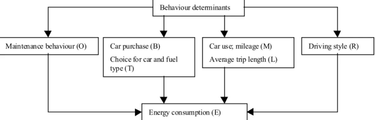
3.7 Blaas et al. (1992)

This report provides a comprehensive overview of the relationships between car ownership, car use and driving behaviour. Figure 3.2 gives an overview of the research field of Blaas et

al. (1992). In this scheme four types of behaviour determining energy consumption are

discerned. These types of behaviour are, in turn, affected by eight behaviour determinants as listed below:

1 Finances

2 Personal characteristics 3 Household situation

4 Geographical spread of living 5 Services and employment

6 Quality and quantity of car infrastructure

7 Quality of services for alternative means of transport

8 Quality of information on the car, and its alternatives and intrinsic motivators (attitudes).

The focus of this study has been placed on the relationship between the eight behaviour determinants and the behaviour types, B, T, R and M. Most conclusions with respect to relationships between costs and ownership, and costs and use, have been mentioned already in Pronk (1991) and Schrijnen (1986). The added value of this study is the more elaborate examination of the relationship between personal characteristics and household composition, and ownership and use. Furthermore, the addition - the examination of the relationship

between information, and ownership and use, signify added value. A chapter in which driving behaviour is studied is also included (as this strongly affects the vehicle energy intensity).

(18)

The impact of the behaviour types on energy consumption has only received limited attention.

Behaviour determinants

Maintenance behaviour (O) Car purchase (B) Choice for car and fuel type (T)

Car use; mileage (M) Average trip length (L)

Driving style (R)

Energy consumption (E)

Figure 3-2 Research field passenger mobility and energy use.

Presentation of the conclusions of this study in matrix form could have given good insight into the relationships if there had not been so many different types of conclusions. The

conclusion with respect to one relationship (e.g. between car use and personal characteristics) contains many remarks, since inclusion of only one remark might give too narrow a view on the considered relationship. Furthermore, the conclusions drawn focus on the intrinsic aspects of the examined relationship to reveal how policy can influence one of the behaviour types. The household situation, for example, turned out to have a significant relationship with car use and ownership. However, this result only becomes interesting if it is known in what way and degree. The authors then argue that men and people from a certain age category show higher car ownership and use since their need to travel (work) is generally greater than for people not belonging to these categories. Another example is the relationship between the quality and the quantity of the public transport network. The author observes a significant relationship. A closer look reveals that especially the competing travel time of alternative modes is an important factor. Public transport often scores poor on this factor because of its organisational fragmentation (connections, waiting times), lower average speed and low network density.

3.8 Johansson and Schipper (1997)

In Johansson and Schipper (1997) the effect of income, price, taxation and population changes on car stock, mean fuel intensity, mean driving distance, car fuel demand and car travel demand is studied. The data used encompasses 12 OECD countries for the 1973-1992 period .

The total demand for car fuel per capita (Q) was defined as the product of car stock per capita (S), fuel intensity (fuel consumption per kilometre driven) (I), and mean driving distance per car per year (D):

Q ≡ S ⋅ I ⋅ D

The three equation variables are modelled separately, which giving the obvious advantage of studying how large a fraction of a long-run change in fuel demand (caused by a change in fuel price) is the result of a decrease in the size of the vehicle stock, a decrease in mean fuel

(19)

intensity and a decrease in mean driving distance per car. However, a disaggregation is much more demanding regarding data. The limited data set has been used as efficiently as possible by focusing on pooled cross-section time-series models. With respect to interdependency of the equation variables, only mean driving distance per year (D) has been estimated as a function of S and I (and other variables: fuel price, income, taxation and national population density). S and I are only dependent on other variables, providing the possibility to use a recursive system instead of a simultaneous equation approach. The results of this study are presented in Table 3-2.

Table 3-2 Approximate range of the rstimated long-run parameters from regressions, including indirect effects ["best guess" in parentheses]4

Estimated

component Fuel Price

5 _Income _{Taxation (other than}

fuel)6 Population density

7

Car stock -0.20 to 0.0 0.75 to 1.25 -0.08 to –0.04 -0.7 to –0.2

[-0.1] [1.0] [-0.06] [-0.4]

Mean fuel intensity -0.45 to –0.35 -0.6 to 0.0 -0.12 to –0.10 -0.3 to –0.1

[-0.40] [0.0] [-0.11] [-0.2]

Mean driving distance

(per car per year)

-0.35 to –0.05 -0.1 to 0.35 0.04 to 0.12 -0.75 to 0.0

[-0.2] [0.2] [0.06] [-0.4]

Car fuel demand -1.0 to –0.40 0.05 to 1.6 -0.16 to –0.02 -1.75 to –0.3

[-0.7] [1.2] [-0.11] [-1.0]

Car travel demand -0.55 to –0.05 0.65 to 1.25 -0.04 to 0.08 -1.45 to –0.2

[-0.3] [1.2] [0.0] [-0.8]

3.9 Kenworthy and Laube (1999)/Dudson (2000)

In Kenworthy and Laube (1999) arguments are introduced for the strong relationship between car use in urban regions/cities and urban density. On the basis of data from 47 cities

throughout the U.S., Europe and Asia, the authors show that 85% of the variance in transport energy use in cities can be explained by urban density, and that there is no evidence to determine a city’s wealth as an explanatory value8. The authors conclude that to enhance the role of public transport in transport energy conservation and to reduce overall transport energy use, cities need to strategically increase their densities of development and improve their degree of centralisation.

4_{What Johansson and Schipper consider as most reasonable on the basis of regressions, knowledge of data}

limitations and statistical methods, and experience

5_{The average price of petrol and diesel fuel, weighted with the actual quantities used by cars and light trucks,}

from IEA (1978-1992) and an unpublished survey by the USA Department of Energy (1973-1978). Prices have been converted to real local 1985 currency using the domestic consumer-price indices. OECD purchasing power parities (PPP) exchange rates have been used to convert all different currencies to 1985 U.S. dollars.

6_{Defined as the sum of different kinds of purchase taxes and import fees plus the present value (on the basis of}

15 years and a real interest rate of 6 per cent) of the annual tax for a specific car, a medium-sized standard car of Volkswagen Golf type.

7_{National population density (citizens per km}2_).

8_{The relation derived from this study is consequently only able to say something about the expected transport}

activity or transport energy use on a given moment at a given urban density. To examine the effect of a rising (or falling) GDP on the energy consumption of urban passenger transport (or on transport activity), cities with similar densities but with different GDP should be analysed.

(20)

Dudson (2000) rejects the recommendations of Kenworthy and Laube (1999) on how urban form policy should contribute to reducing urban transport energy use. The author argues that in order to achieve substantial transport energy reduction, efforts must not be placed on improving public transport or redeveloping cities, but that attention should be paid to new technologies (fuel injection, hybrids) and alternative fuels (fuel cells) with which energy consumption reductions can be achieved of 20% to 75% by the year 2005. Dudson (2000) argues that, under two “extreme” assumptions, the decrease in energy use due to geographical planning is only marginal. If public transit consumes 40% less energy per passenger per km than cars and if, “beyond reasonable expectations”, the use of public transit doubles from 3% to 6% of motorised urban transport, the energy reduction potentially possible in U.S. cities will be no more than 1.5%. On the basis of these findings the author concludes

(re)developing urban form to be ineffective “within the timeframe of a potential new oil crisis” (since substantial city growth will take several decades) and emphasis should be placed on the implementation of new technologies.

3.10 Literature – subjects overview

Table 3-3 Literature sources and topics discussed in relation to transport activity/energy consumption Source/ Determinant Technol og y Po licy U rban F orm / P lanni ng C ar ow ners hi p Ca r u se CO 2 em issio n Elasticitie s Ti me/ m oney cons tr ai nt Schipper (1997) X XX X Blijenberg and Van Swigchem (1997) X XX X X Banister (1996) XX Dargay and Gately (2001) XX Schrijnen (1986) X XX XX Blaas et al. (1992) X XX XX Pronk (1991) X XX XX Johansson and Schipper (1997) XX Kenworthy and Laube (1999) X XX

XX: Focus of considered source

(21)

4. Global transport models

In this chapter, five global transport models are presented on the basis of available information about these models. Except if explicitly mentioned, this chapter does not represent the view of the author.

4.1 IEA Model and income & price elasticities - Wohlgemuth

(1998)

4.1.1. Methodology

This paper presents the IEA’s approach of modelling transport energy demand. Fuel demand, which is not a demand per se, is derived, whenever possible, from the economic activity in the transport sector and not estimated directly, i.e. using one equation or a (simultaneous) equation system. In general, the transport models employ a “two-step approach”. In the first step, transport activity, the sector’s relevant energy service, is estimated econometrically. In the second step, the transport activity projections are then combined with estimates of efficiency improvements, car turnover rates and diesel/gasoline penetration assumptions to arrive at projections of fuel demand. The effectiveness of economic instruments is a function of the reaction of consumers (and businesses) to income and price changes. An in-depth understanding of income and price elasticities of transport demand and transport energy demand is important to be able to assess the effectiveness of policies considered.

4.1.2 Determinants of transport energy demand

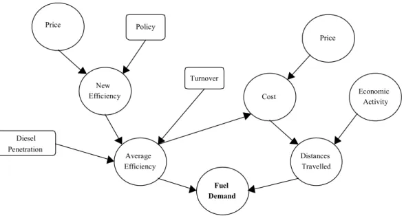
GDP alone proved insufficient to explain variations in transport energy demand. In addition to income other factors like cost of driving, availability and ticket prices for public transit, prices of motor vehicles, quality of the transport infrastructure, settlement structure, social patterns, climatic, physical and geographical conditions and policy measures can play an important role too. Wohlgemuth (1998) emphasises that it is essential to model demand for the various fuel types individually, since the demand is driven by different factors. The demand for diesel fuel is usually closely linked to general economic development, whereas demand for petrol/gasoline and, to a lesser extent, aviation fuels depends much more on available income, demography, weather, fuel prices and taxation. The IEA model applied in this study projects global transport energy demand (passenger and freight) by region and fuel type. Figure 4-19 presents the model as presented by Wohlgemuth (1998).

9_{In section 4.1.4 a more recent version of the IEA model structure is presented. Though, the results of the study}

(22)

New Efficiency Average Efficiency Fuel Demand Distances Travelled Economic Activity Price Cost Price Turnover Policy Diesel Penetration

Figure 4-1 Overview of the IEA transport model.

The weakness of this model is that it has not endogenised the choice of mode of transport (car, bus, rail or aircraft) or the purpose of travel (recreation, work or shopping). The model only projects fuel demand for road transport. It is argued that a more detailed model would require the projection of a larger number of exogenous variables, a requirement that is not compatible with the overall design of the World Energy Model (WEM).

Whenever possible the IEA’s transport model employs the two-step approach. Fuel demand is not directly estimated but if reliable data are available for the region considered, it is derived from the economic activity in the transport sector. The elasticities obtained are a reflection not of the demand for fuels but of the relevant energy services, which are a

combination of energy-related capital equipment (vehicles) and fuel efficiency. The principal advantage of this approach is that the relevant energy services are modelled and that, for model simulation, efficiency improvements, gasoline penetration and car turnover rate can be dealt with explicitly.

4.1.2.1 Importance of income

Income is both in absolute and in per capita terms the most important determinant of transport demand. However, the related energy consumption can vary considerably among countries with equal per capita GDP. Therefore it is expected that the structure of GDP is also important. If the structure of GDP shifts away from heavy towards a lighter industry

(dematerialization), the number of tonne kilometres is expected to decline. However, a contradictory trend might offset the reduced energy consumption induced by

dematerialization, since freight transport energy intensity may increase through a shift to more energy intensive modes of transport (i.e. rail to road). The overall effect on energy consumption is ambiguous.

The share of (incremental) transport energy demand within total final energy demand is also closely linked to the stage of development: the higher the per-capita GDP, the more

(23)

4.1.2.2 Fuel prices and cost of travel

Fuel also has a great effect on transport energy consumption. Gasoline/petrol and diesel prices vary substantially among countries and account for part of the difference in per-capita fuel consumption between regions. In the U.S. people drove farther on cleaner fuels for less money in 1995 than ever before. Real average prices were lower than they were in the entire 80-year period before.

Taxation on vehicle purchases is usually designed to raise governmental revenues instead of improving energy efficiencies. Too high taxes can even have a negative impact on the fleet efficiency because people tend to keep their old (low-fuel efficiency) car as long as possible. Fuel costs are only part of total costs of travel (around 25%), which means that elasticity to total costs is larger than to fuel costs alone. The elasticity will depend on the time period, trip purpose, method of charging the absolute level of price changes and the income level. It is found that the elasticity is lowest for business trips, higher for commuting to work and highest for shopping and leisure activities.

4.1.2.3 Fuel economy

Energy consumption is not only dependent on transport mode but also on the way the mode is managed. In general, lifestyle and car driver behaviour have great influence on fuel economy. Short trips in the city usually consume more energy per kilometre than longer non-urban trips due to the lower level of congestion and less frequent acceleration and braking. The last few years a trend has been seen of consumers tending to prefer heavier, more comfortable and more powerful cars, which partly offsets fuel savings by technological progress. The average fuel economy (i.e. use of fuel) has also been increasing due to the declining vehicle

occupancy. Possible policy measures could involve higher fuel taxes or higher minimum standards of average fuel economy.

4.1.3 Elasticity estimates

Many researchers have been doing studies on transport fuel demand elasticities. However, the common feature is that there is little consistency in methodology and assumptions among the various studies. The study pesents a few price elasticities. A comprehensive summary of price elasticities from Goodwin (1992) suggests that traffic volume elasticities with respect to fuel prices are –0.16 in the short term and –0.33 in the long term. The short-term elasticity on fuel consumption is probably around –0.27 and, in the long term around –0.71 when using time-series estimates. Elasticities derived from cross-section data tend to be higher on average: -0.28 in the short term and –0.84 in the long term.

Fuel consumption elasticities can be expected to be greater than traffic demand elasticities because, in the long term, changes in the fuel economy and vehicle characteristics (motor power, weight) can be expected to have an effect on fuel consumption while preserving mobility. A price increase may thus cause lower fuel consumption while the distance travelled does not decline.

4.1.4 Demand elasticities in the OECD transportation sector

4.1.4.1 Road passenger transportation

Distances travelled by passenger cars and light trucks have been estimated for the United States, OECD Europe and Japan. Determinants for estimates of road passenger transportation activity are income, cost of travel and population. Income is approximated by consumer expenditures (per capita in U.S case); fuel prices and fuel efficiencies are used as proxies for

(24)

costs of travel. The estimated distances travelled, together with assumptions and estimates of efficiency improvements, penetration of diesel cars and average life of cars give the projected fuel demand (see Figure 4-1 Overview of the IEA transport model).

Appendix 2 Table A-15 shows the long-term OECD transportation demand elasticities. The lower elasticity in the U.S. could be explained by the higher saturation of road transport. Also, the estimation is on a per capita basis. When estimating the levels, the implied long-term income elasticity increases to 0.93. Price elasticity remains almost unchanged at -0.14

10_{. It is notable that the large fuel efficiency improvements in the U.S. have had a big}

influence on income elasticity. If the fuel efficiency variable was omitted, the income elasticity increased from 0.88 to 1.06 in the per-capita case and from 0.93 to 1.04 when estimating levels. The increases of the elasticities correspond well with estimates of Greene of the rebound effect (0.15). The higher elasticities for Europe are explained by the better public transport system in Europe, allowing for more substitution. Price increases force people more quickly into using public transport. It should be noted that in the model the cost of travel is determined by the price of gasoline only. If the diesel price is used instead of the gasoline price, the long-term price elasticity falls to –0.56, still much higher than either in the U.S. or Japan.

Appendix 2 Table A-16 shows elasticities obtained from estimations based on a consistent database. In this case, the level of distances travelled for distances travelled in all three regions is estimated using consumer expenditures, the gasoline price and omitting the fuel efficiency variable. In Appendix 2 Table A-17, the short-run (first year, 1967) OECD

transport demand elasticities are presented. The difference between the values for Europe and the U.S. is remarkable.

4.1.4.2 Freight transportation

The dependent variable in freight transportation is tonne kilometres for Europe and Japan and tonne miles for the U.S. In case of Europe and U.S., truck freight kilometres have been estimated indirectly via total estimated freight volume and the share of truck-moved freight. In the case of Japan, truck tonne kilometres have been modelled directly.

GDP reflects economic activity and the relative costs of travel are reflected by the real price of diesel. The resulting income elasticities are close to 1 for U.S. and Europe, while 1.4 for Japan. If elasticities are modelled directly for U.S. and Europe, elasticities rise respectively to 1.13 and 1.37. The reason for this difference probably lies in the fact that road transportation grows faster than rail transport. The modal split is affected by the value-to-weight ratio. Generally, an increasing ratio means a shift from rail to road transportation. In all three regions the long-term price effect is approximately – 0.2.

4.1.4.3 Air transportation

Due to lack of reliable data, only fuel consumption of U.S. air travel has been estimated with the underlying variables of passenger air miles and costs of travel (broader than fuel costs only). The fuel consumption of air travel in Japan and Europe has been estimated directly (cross-sectional or time-series). The underlying income variables are consumer expenditures for Japan and Europe, and GDP in the case of the U.S.. The resulting long-term elasticities of 1.35 for Europe and 1.8 for Japan and the U.S. probably reflect the luxury nature of air travel.

10_{Note by the author: however, the relative change is only 5.3% for the income elasticity and 12.5% for price}

(25)

The fuel price elasticities, based on the costs of crude oil, are -0.03 and –0.09 for Japan and Europe, respectively. The price elasticity of the U.S., reflecting total costs of travel, is much larger than the elasticities of Japan and Europe at -0.34. One can expect price elasticities based on primary price series to be less sensitive than those based on end-use prices because of the often weak links between these two prices. However, even end-use prices of fuels usually do not properly reflect the cost of travel since the fuel-cost component of the different modes of transportation can be very low compared to total cost of travel. In the model, the fuel price of air transportation in the U.S. in 1993 amounted to less than 20% of total cost of air travel. In cases where crude oil prices in the U.S. case are used, U.S. price elasticity falls to –0.055, much closer to the values of Japan and Europe.

4.1.5 Travel/fuel demand elasticities in non-OECD regions

Estimation of fuel demand elasticities in non-OECD countries has been performed with simpler methodologies since data availability is low. A cross-sectional approach has been used to analyse the income and price elasticities for numerous non-OECD countries due to lack of consistent time-series. Another reason for using cross-section techniques lies in the fact that it is intended to reveal long-term equilibrium relationships. Many of the problems related to obtaining good estimates for income and price elasticities arise because of lags between changes in the dependent variable and the corresponding exogenous model variables (i.e. slow vehicle turnover rates). When employing a time-series approach, a feasible dynamic specification, which is reflected in a specific lag-structure, has to be imposed. Use of a cross-sectional approach can avoid this by assuming that the estimates immediately reflect long-term relationships.

Appendix 2 Table A-18 show the long term non-OECD transportation (fuel) demand elasticities. The type of methodology and the underlying dependent variables are also

presented. In the regions for which no time-series data are available, the elasticities have been derived using cross-section analysis. The elasticities and the underlying assumptions are shown in Appendix 2 Table A-19.

4.1.6 Projections

The model projects a rapid increase in passenger and freight traffic and the corresponding transport energy demand, which is likely to lead to pressures on transport policies. In many regions of the world it is recognised that demand management tools such as road pricing and telematics will have to play a prominent role in the future to control transport volumes. The largest concerns/weaknesses of this model are the non-endogenised variables “choice of mode”, “purpose of travel” and non-incorporation of the costs of potential substitutes, although the effects of the latter probably are only moderate since a large proportion of driving is non-discretionary. However, estimating the cost of travel presents a major problem, at least in the long term, since it should include the lifetime costs of owning and operating a car. Even the short-term cost of travel is not only determined by the costs of fuel but should take into account the fuel efficiency of the car and other variable costs as well. The above-mentioned model restrictions and weaknesses may have led to uncertain results.

The projections of the IEA model for the increase in transport and the fuel demand are presented per region in Table A-20 Appendix 2. This IEA model projects an average annual growth rate in the transport energy consumption of 2.6% per year (over 1993-2010).

(26)

4.1.7 IEA model

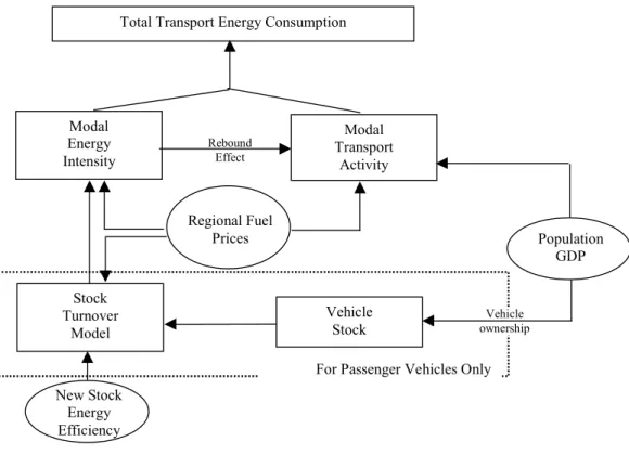
Figure 4-2 presents the renewed transport model structure of the IEA. The old econometric approach is combined with a recently developed bottom-up approach because the policies described in chapter 11 of IEA (2000) require a more disaggregated framework than provided by the standard World Energy Model. The structure presented is thus not obtained from Wohlgemuth (1998) but from Appendix 1 of the World Energy Outlook 2000 IEA (2000). For every region, activity levels for each mode of transport are a function of population, GDP and price. The elasticity of transport activity to the fuel costs per km is applied to all modes except passenger and freight rail, and inland waterways. In the case of passenger vehicles, this elasticity is also used to determine the rebound effect of increased transport demand resulting from improved fuel intensity. Other assumptions to reflect passenger vehicle ownership are also made.

Modal energy intensity is projected by taking into account changes in energy efficiency and fuel prices. Explicitly, stock turnover for cars and light duty vehicles is modelled in order to allow for the effects of fuel efficiency regulation of new cars on fleet energy intensity. Fuel efficiency regulation and additional fuel taxation can be directly modelled.

This model projects that in 2020, 120 EJ will be used in the transport sector, which corresponds with an average annual growth rate of 2.4% (1997-2020).

Figure 4-2 IEA transport model structure.

Rebound Effect Vehicle ownership Modal Transport Activity Modal Energy Intensity Regional Fuel Prices Stock Turnover Model Population GDP Vehicle Stock

For Passenger Vehicles Only Total Transport Energy Consumption

New Stock Energy Efficiency

(27)

4.2 Model: World Energy Council (1995)

Over the past years, the World Energy Council (WEC) has developed a global transportation model. The initial model, covering car, road/rail freight, and aircraft transport, is used to project the transport activities through 2020 (World Energy Council, (1995). Explicit scenarios were developed to examine how the world’s total energy use might be radically altered either by more robust economic growth or by a radical change in priorities favouring increased environmental protection.

4.2.1 Introduction

The global transport model used in the World Energy Council (1995) has been developed within Statoil Corporate Planning for the primary purpose of producing the quantitative scenario assessments for the WEC transportation project. This model actually emphasises passenger road transport; due to lack of data for other sectors, it was not considered

meaningful to construct a detailed model for freight and air transport. Results from this model are generated with scenario analysis through the year 2020. Three different scenarios have been designed, each attributed with a different projection of economic and technological development, oil supply, environmental awareness, government/market involvement (regulation) and lifestyle changes.

4.2.2 Determinants

The WEC report determines economic growth as the most important determinant of transport energy demand but suggest that this apparent stable link between GDP and transport demand might be broken by “dematerialisation” (ever-growing importance of the service sector) and the global trend towards economic liberalisation and internationalisation of trade11. Notable is the impact of liberalisation of the oil market, since it can have a great effect on the incentive to develop energy-efficient or alternative technologies for vehicle propulsion. Due increasing competition the oil price will fall and still the demand of oil will be met. The incentive for technological development will decline.

Secondly, the report mentions demographic trends as another vital factor affecting future transport demand. Not only population growth, but also age structure, urbanisation and household size and composition have been examined. The most important demographic factor is the declining fertility affecting household size. The most important social factor is the decline in the three-generation families and the reduction in the proportion of married couples in the population. The most important economic factor is the increased affluence and the growing economic independence of women and young people. The fragmentation of families and the associated loosening of family bonds will result in a growing demand for mobility.

11_{The suggested possible decoupling of GDP and transport has so far not been seen. This is explained in the}

same reference: Already in the early 1980s, it was generally expected that freight transport in the industrialised countries would grow only very slowly because of the relative decline of heavy industry. The assumption was, of course, that growth in the service sector would require less freight transport than growth in the industrial sector. So far, however, the forecasts have been wrong. Actually, the fact that ECMT freight volumes grew rapidly from the mid-1980s can largely be explained by economic liberalisation. This compensatory factor has lead to a spatial redistribution of the economic activities of production and distribution, built on national and international specialisation, which in turn has resulted in longer distances for freight transport.

(28)

Environmental concerns12 are the driving force behind many of the transport sector regulations. The most efficient way of abating these environmental problems is through measures constraining the demand for transport or by developing new fuel-efficient

technologies, although alternative fuels and reformulated gasoline will also play a role. Side-effects of measures taken will, however, redistribute the costs in society. Policy-makers will not only have to look at the merits of transport regulation but also take into account the interest of various stakeholders.

Changes in lifestyle could have a fundamental impact on future transportation demand. Today, the car serves as an important transportation device but also as a symbol of welfare. In the future, lifestyle changes could be linked to increased environmental awareness or continued dramatic progress in the field of advanced telecommunication. However, the impact is likely to vary substantially among different regions in the world. The introduction of telecommuting, for instance, has been relatively faster in the U.S. than in other

industrialised countries.

Fuel efficiency and alternative fuels are determinants related to the more exogenous factor “technology”. With time, technology improvements will enable introduction of more fuel-efficient motors or motors using alternative fuels like ethanol at a competitive price. The car industry is in this respect easier to adjust than the aircraft industry. Potential alternative fuels for gasoline in the car industry are ethanol, hydrogen, LPG, rape-seed oil, electricity and methanol (of which natural gas (LPG) has the best odds within the given time framework: year 2020). The practical possibilities of the implementation of the possible alternative fuels (natural gas and liquid hydrogen) in the aircraft industry is low. This is due to a lack of technology, as well as to the gigantic investments in aircraft and infrastructure for the refuelling at the airports.

4.2.3 The model

The model configured for the description of passenger road transport is as indicated in Figure 4.3.

12_{Author’s note: In the report, environmental concerns are also taken up in the same chapter. However, the}

negative impact of environmental pollution due to increased transport, will probably not affect transport demand autonomously (in contrast to GDP, for example). Since the effects of environmental pollution (read emissions) are long-term ones, the gravity of the resulting problems (e.g. lung diseases, reduced learning ability) for the population is often unclear. If the impact of a certain event is apparent, the awareness among people will be greater and also their response. An example mentioned in World Energy Council (1995), was the increased death rate, probably due to increased NO2 levels in London in 1991. Statistics showed a 10% increase, though it

is doubtful whether the London population was really aware of the cause of it. In this way, environmental pollution will probably not have a great mitigating effect on transport demand. Pollution merely figures as an incentive for governments to search for solutions.