Implementation of source apportionment using Positive Matrix Factorization - Application of the Palookaville exercise

(1)

RIVM Report 863001006/2007

Implementation of source apportionment using Positive

Matrix Factorization

Application of the Palookaville exercise

D. Mooibroek R. Hoogerbrugge H.J.Th Bloemen

Contact: D. Mooibroek

Laboratory for Environmental Monitoring dennis.mooibroek@rivm.nl

This investigation has been performed by order and for the account of Ministry of Housing, Spatial Planning and Environment, within the framework of project M863001 Air Pollution and Health.

(2)

Parts of this publication may be reproduced, provided acknowledgement is given to the 'National Institute for Public Health and the Environment', along with the title and year of publication.

(3)

Abstract

Implementation of source apportionment using Positive Matrix Factorization

Particulate Matter (PM) has been recognized for its association with an increase of cardio-respiratory diseases as well as premature mortality (shortening of life time). It is important to determine which sources contribute to the emission of PM in order to facilitate and support the development and implementation of emission reduction policies. Emissions from a mixture of sources, which vary per location and over time, contribute to the concentration of ambient PM

Rather than attempting to identify the critical chemicals or physical properties that are responsible for the adverse effects of PM, it may be more effective and expeditious to identify the contributing sources. The RIVM has implemented a source apportionment methodology to quantify the relative contributions of various sources to PM. The data on these source contributions provided by this methodology can be used by the Ministry of Environment in developing an abatement strategy for PM.

Various complex mathematical models have been developed that use measurements to provide a better insight into the relative contributions of sources. An example of such a model is the Positive Matrix Factorization (PMF), which has been used in this study. To acquire the necessary expertise, the RIVM has applied the PMF to a well-defined reference dataset, known as the Palookaville dataset, which consists of simulated measurements.

The Palookaville dataset contains deliberate inconsistencies, all of which were found during the analysis. The capability of the RIVM to detect these inconsistencies using the PMF demonstrates that the RIVM has developed a sufficient understanding of the techniques involved to apply the PMF model to other datasets.

Key words:

(4)

Rapport in het kort

Implementatie van brontoewijzing door gebruik te maken van Positive Matrix Factorization De negatieve gevolgen van fijn stof op de volksgezondheid, zoals een toename van luchtwegziekten en vroegtijdige sterfte, zijn onderkend. Om sneller passende beleidsmaatregelen tegen de uitstoot van fijn stof te kunnen bepalen en toe te passen, is het belangrijk te achterhalen welke bronnen aan die uitstoot bijdragen en wat de bijdrage van die bronnen is aan gezondheidseffecten. Uitstoot van verschillende bronnen, variërend per locatie en tijd, draagt bij aan de concentratie fijn stof.

Deze werkwijze is effectiever dan uit te zoeken welke chemische onderdelen of fysische eigenschappen van fijn stof verantwoordelijk zijn voor deze negatieve effecten. Het RIVM heeft een methode

uitgewerkt waarmee de relatieve bijdrage van bronnen in kaart kan worden gebracht. Het ministerie van VROM kan deze inzichten gebruiken in zijn strategie om de uitstoot van fijn stof te verminderen. Er bestaan complexe rekenkundig modellen die op basis van metingen de relatieve bijdrage van deze bronnen kunnen achterhalen. Een voorbeeld van zo’n model is ‘Positive Matrix Factorization’. Om de benodigde expertise op te bouwen heeft het RIVM dit model toegepast op beschikbare

referentiegegevens, bekend als de Palookaville-data, opgebouwd uit gesimuleerde metingen.

Tijdens de analyse zijn de inconsistenties die opzettelijk in deze dataset zijn aangebracht, aan het licht gekomen. Hierdoor heeft het RIVM aangetoond voldoende inzicht te hebben in de

brontoewijzingsmodelering om het gebruikte rekenmodel toe te passen. Trefwoorden:

(5)

Acknowledgements

The authors would like to thank Shelly Eberly, Tom Coulter, Charles Lewis and Gary Norris of the U.S. Environmental Protection Agency for providing the data and for the interesting discussions about source apportionment. We would also like to thank Dr. P. Paatero of the University of Helsinki and Dr. P.K. Hopke of the Clarkson University for the useful discussions on the use of Positive Matrix Factorization. Last but not least we would like to thank Dr. Ron Henry of the University of Southern California for the useful discussions on UNMIX.

(6)

(7)

3.2.3 Assignment of source types using elemental composition 26 3.2.4 Assignment of source types using meteorological data 29 3.2.5 Differences between the assignments of source types 32 3.2.6 Mass apportionment for the ten-factor solution 33 3.3 Comparing the results with the known contributions 35

3.4 Conclusion of the Palookaville exercise 36

4 Conclusion 39

5 General points of interest 41

5.1 Handling missing data and data below the MDL 41

5.2 Estimation of the standard deviations 41

5.3 Inclusion of species in the model 41

5.4 Determining the number of factors 42

5.5 Identification based on elemental composition 42

5.6 Identification based on wind-directional analysis 42 5.7 Other publications using the Palookaville dataset 42

(8)

References 43

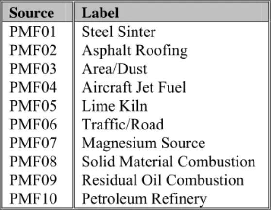
Appendix 1 Overview of selected SPECIATE profiles 47

Appendix 2 Contributions 51

(9)

Summary

Recent years has seen an increased interest in source apportionment studies of particulate matter (PM), largely as a result of the growing awareness that PM has a negative effect on human health. This increased awareness has led researchers to focus on the relative contributions of different sources (both natural and anthropogenic) to PM levels on both the local and regional scales. The identification and quantification of these sources provide both important background data for the formulation and implementation of reduction policies and valuable information on their effects on human health. To date, it remains unclear which particle types/sources are the most responsible for this association (Thurston et al., 2005).

Since the early 1970s various research approaches have been used to identify sources of ambient fine PM – with varying degrees of success (Miller et al., 1972; Friedlander, 1973; Hopke et al., 1976). A better understanding of the underlying mathematical problems involved in source apportionment has led to a specific modeling field, referred to as receptor modeling, in which various models have been developed on the basis of different principles. All receptor models require both considerable

background knowledge and expertise to be understood and used properly. The aim of this study reported here was to gain the expertise and understanding necessary to perform source apportionment using an available receptor model.

Based upon initial trail runs with various receptor models Positive Matrix Factorization (PMF) was found to be the most promising model currently available. The PMF model has been applied to a well-defined reference dataset provided by the US–EPA, consisting of simulated measurements in an imaginary town called ‘Palookaville’. The analysis was performed without any prior knowledge of the constituent source information. The results of the analysis, source profiles and time profiles together with some unusual discrepancies were reported to the US–EPA, which then sent back a description of the dataset together with discrepancies that had been deliberately built into the dataset. The evaluation was used to determine if a level of expertise and understanding for applying source apportionment has been achieved by comparing the results with the parameters used to construct the dataset.

Expertise in the field of receptor modeling was initially acquired from various literature studies and visits/discussions with researchers working in this field. Detailed information on the steps necessary to perform source apportionment with the PMF model is given in Chapters 2 and 5. Based on information extracted from the literature studies, we developed various self-made analytical tools to facilitate the analysis of the results provided by PMF.

The sources and their contributions that were calculated using the PMF model for the reference dataset are in good agreement with the contributions used by the EPA to construct the dataset. The results were also compared to those of a study carried out by Hopke (cited in Willis, 2000). Based on the different data pre-treatment in both studies slight differences were found in both the number of sources and the source contributions.

Based on the results of this study we have sufficient confidence in the Positive Matrix Factorization technique itself and in our level of experience for applying it on real datasets.

(10)

(11)

1 Introduction

Source apportionment studies of particulate matter (PM) have received increasing attention in recent years as it has become increasingly recognized that PM has adverse effects on human health. The increased awareness of these health effects has led researchers to focus on the relative contributions of different sources (both natural and anthropogenic) to PM levels on both the local and regional scales. An understanding of the relative contributions of these sources is important for the formulation and implementation of reduction policies and for an understanding of their effects on human health. To date, it remains unclear which particle types/sources are the most responsible for this association (Thurston et al., 2005).

Since the early 1970s various research approaches have been used to identify sources of ambient fine PM, all with varying degrees of success (Miller et al., 1972; Friedlander, 1973; Hopke et al., 1976). A better understanding of the underlying mathematical problems involved in source apportionment has led to a specific modeling field, referred to as receptor modeling, in which various models have been developed based on different principles. All of these receptor models require both considerable background knowledge and expertise to be understood and used properly.

The aim of the study reported here was twofold: (1) to gain the expertise and understanding necessary to perform source apportionment; (2) to determine if the necessary level of expertise has been achieved by evaluating an available receptor model, the Positive Matrix Factorization (PMF) model. Here, we provide detailed information extracted from various literature studies. In addition, using a synthetic dataset developed by the U.S. Environmental Protection Agency (EPA) and provided with detailed information on the construction of this dataset, we evaluate this model to determine whether a level of expertise for applying source apportionment has been achieved.

1.1 Basic assumptions in receptor modeling

It is a self-evident fact that all receptor models, similar to all models, are an imperfect replica of the real-life situation. Since not all of the important variables or the interaction between variables can be specified in any one model, a model remains only an approximation of reality. However, as our understanding of the complex real world increases, models can be improved to provide a better description of reality (Watson, 1984).

Three basic assumptions must be made in order to describe reality using mathematical functions. For receptor modeling, these assumptions are:

Assumption 1: Composition of source emissions is constant

Assumption 2: Components do not react with each other (i.e. they add up linearly) Assumption 3: p (-identified or unknown) sources contribute to the receptor

These three basic assumptions underlying receptor modeling will not be fully valid in real-life situations because: (1) the source compositions are not constant (e.g. changes in source compositions can occur during different emission cycles), (2) components do react with each other and systems are not linear and (3) the number of sources which contributes to a receptor is not known.

(12)

Many sources commonly have similar contributions, which will make it difficult to distinguish these sources. In addition, very few sources have unique tracer components. If these assumptions do not hold, one may ask why receptor modeling should be used. Watson (1984) provides one answer to this dilemma when he states that the fulfilment of an assumption is not merely a question of true or false but usually in its degree of correctness (Watson, 1984). For example, the assumption of a constant composition of source emissions is true more often for a PM source than for a gaseous source.

In most cases, deviations from the basic assumptions can be tolerated within the goal of the application, but the quantification of these deviations must remain an important aspect of the application.

1.2 Commonly used models

In the field of receptor modeling there are two basic approaches to the problem, depending on the information available on the number and nature of the sources. When the sources are known and the compositions are either measured or otherwise available, the Chemical Mass Balance (CMB) approach would be the most appropriate.

To facilitate the search for the chemical source compositions of various known sources the US–EPA has developed a repository of speciated profiles for total organic compounds (TOC) and PM for a variety of sources for use in source apportionment studies. This repository is referred to as the SPECIATE database. The objectives of the SPECIATE database are (1) to identify chemical and physical characteristics of primary PM and volatile organic compound (VOC) emissions; (2) to tabulate and document fractional the abundances and variabilities of specified chemical and physical

components in primary PM and VOC emissions; (3) to provide a data interface to receptor source apportionment models and speciated emission inventories (Watson and Chow, 2002). The main disadvantage of the SPECIATE profiles is the lack of universally applicable source profiles. A source profile detailing the chemical composition of a traffic source in the United States may not be applicable for a traffic source in Eastern Europe.

However, in most practical cases, no prior information is available on the sources located in the receptor area, and the user is faced with the difficult task of searching out the relevant sources. Models used in earlier studies for solving this problem include Principal Component Analysis (PCA) and Factor Analysis (FA). However, these models were found to be less suitable for the use of receptor modeling (Paatero and Tapper, 1994). Two different models were subsequently developed based on either Self-Modeling Curve Resolution (SMCR) (Lawton and Sylvestre, 1971; Henry, 1997) or on least squares minimization (Paatero, 1997a,b).

A brief description of three mainstream models for each of the aforementioned approaches is provided below.

1.2.1 Chemical Mass Balance model

The CMB was first proposed for aerosols in the early 1970s (Miller et al., 1972; Friedlander, 1973). The model assumes that the selection of measured species at a receptor site is a linear combination of species contributed by known profiles from independent sources – i.e. for each of the samples the

(13)

the receptor point have been identified and that the compositions of each source is known. Fulfilment of this assumption requires detailed knowledge of both the sources in the area of the receptor and of the source compositions of each source.

1.2.2 UNMIX

UNMIX, which is based upon SMCR principles, is a type of factor analysis that imposes a non-negative constraint for the generation of more physical meaningful source contributions and profiles. The model is based upon two key algorithms with the Singular Value Decomposition (SVD) as a link between them. The first algorithm, NUMFACT (Henry et al., 1999), estimates the number of sources that can be resolved relative to the ambient dataset based on signal-to-noise ratios (Lewis et al., 2003). The other algorithm finds data ‘edges’ that are closely related to the contributions and compositions of sources in the more dimensional spaces. For more details on the mathematical aspects of the UNMIX model, the reader is referred to Henry (2003).

1.2.3 Positive Matrix Factorization

Positive Matrix Factorization (PMF) is based upon least squares minimization and was developed by Paatero and Tapper (1993, 1994). Based on mathematical differences between the three mainstream models and the results of some preliminary trail runs with each model, we decided to use PMF to evaluate the EPA synthetic dataset of the imaginary town of Palookaville. The principles of this model are discussed in more detail in Chapter 2 Methods and Materials. The PMF model has been greatly improved since its initial development, resulting in the Multi-linear Engine (Paatero, 1999) and, more recently, in the EPA–PMF model (Eberly, 2005).

The results of our evaluation of the synthetic dataset using PMF are compared to the results of various other studies to determine if the required level of expertise needed to perform source apportionment with PMF has been achieved.

(14)

(15)

2 Methods and Materials

2.1 Dataset

The dataset used in this study is a synthetic dataset developed by the EPA Office of Air Quality Planning and Standards (EPA–OAQPS) and was used in the Workshop on UNMIX and PMF as applied to PM2,.5,held on 14–16 February 2000 in Research Triangle Park, North Carolina, USA

(Willis, 2000).

The simulated measurement data consist of daily PM2.5 samples for a period of 1 year (1984) at a

receptor site located in the imaginary town of Palookaville. Each sample was characterized by the concentrations of 50 chemical species: Al, NH3, Sb, As, Ba, Bi, Br, Cd, Ca, CO32-, Cs, Cl-, Cr, Co, Cu,

EC (Elemental Carbon), Ga, In, I, Fe, La, Pb, Mg, Mn, Hg, Mo, Nd, Ni, Nb, NO3-, OC (organic

carbon), Pd, P, K, Pr, Rb, Se, Si, Ag, Na, Sr, SO42-, S, H2SO4, Sn, Ti, V, Y, Zn, and Zr. The total PM2.5

mass concentration for each sample was also provided.

The Industrial Source Complex Short-Term (ISCST3) Dispersion model was used to simulate the daily PM2.5 samples. The ISCST3 model is a widely used steady-state Gaussian plume model that can be

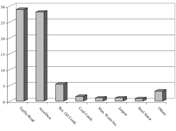
used to assess non-reactive pollutant concentrations from a wide variety of source types that are associated with various simulated situations – in this case, a simulated town. Modeling options include algorithms for calculating air pollution concentrations due to the dry and wet deposition of particles, building downwash, plume rise as a function of downwind distance, separation of point sources, limited terrain adjustment and emissions from area, line and volume sources (Atkinson et al., 1997). Sixteen distinct source profiles were used as input for the ISCST3 model: nine point sources, four industrial complexes, one area source and two highways. Hourly meteorological data, including wind speed and direction, completed the dataset. An overview of the used source profiles is given in Table 1. The area source profile used here contained a mixture of dust and road profiles. The petroleum refinery had some built-in variability [coefficient of variation (CV) of approximately 25%], while all other source profiles were fixed. Temporal modulation of the source strengths (50% CV for most) was found to be essential for resolution of the sources (Willis, 2000).

Five of the nine point sources were modeled to have seasonal variations, and two others were modeled to have weekly variations. Both highways were modeled to have weekly and holiday variations. In addition to variations in emissions, the variation induced by the hourly meteorological data, obtained at a National Airport, Washington D.C. in 1984, was also included.

Table 1 An overview of the sixteen source profiles used in the dataset. Source profiles used in Palookaville dataset Lime Kiln, Wood combustion, Coal combustion, Glass Furnace,

Metal fabrication, Iron ore dust, Municipal incinerator, Residual oil combustion, Petroleum Refinery, Cement products, Asphalt roofing, Steel sinter, Jet fuel. Two roads (DRI + road dust), one area profile (= a mix of dust and roads)

(16)

0 5 10 15 20 25 30 avg. c o n tr ib u ti o n ( µ g/ m 3 ) Tr af fic/_Ro ad Ar ea/D ust Re s. O il C om b. Co al Co m b. M un._W aste Inc . Airp or_t Ste el Si nter Ot he rs

Figure 1 Average source strengths for each source in the Palookaville area.

Each of the aforementioned 50 chemical species had a single minimum detection limit (MDL) and a single uncertainty, which were fixed across the entire dataset. A random number between 5% and 10% was chosen for each species and used as the CV for the log-normal distribution of the measurement error of that species. A daily random measurement error was drawn from this log-normal distribution and applied after the ‘true’ species concentration at the receptor had been computed.

A single MDL for each species was computed as the maximum of 1.5 × CV × (mean concentration) and 0.001 μg/m3_{. The data below the MDL were not modified in any way (Willis, 2000).}

As well as monitoring data, information was provided on the corresponding MDL and uncertainties for the town layout, meteorological data and source profiles originating from the SPECIATE database. In Figure 2, which is provided as part of the metadata by the EPA the locations of the main sources relative to the receptor point are displayed on the map of Palookaville. The green ‘star’ in the middle of the city is the monitoring site. The dashed box encloses the urban area, and the two lines represent major roadways.

(17)

The major sources in the Palookaville area are: • Southwest of city: cement production

• Southwestern area of city: combination of asphalt roofing manufacturing, glass furnace, metal fabrication, steel sinter and iron ore dust sinter.

• Eastern area of city: wood combustion

• Northern area of city: airport, residual oil combustion, and petroleum refining • Northwestern area of city: lime kiln

Figure 2 Location of the main sources relative to the receptor location [as provided at the workshop (Willis,2000)]

(18)

2.2 Positive Matrix Factorization

2.2.1 Introduction

As mentioned in the Introduction, both PCA and FA are well-known methods for solving a bilinear model. These methods have been very successful in some fields but have found limited application in the physical sciences (Paatero and Tapper, 1994), primarily due to the inherent possibility that negative amounts will be a basic constituent in almost all factors. In the physical sciences, the non-negativity constraint is a natural phenomenon, and this constraint should be obeyed by the factor model. Another significant drawback to these methods is the rotational indeterminacy in the solution. This problem can be solved, but it does not produce a unique solution (Paatero et al., 2002b) and, in fact, multiple valid solutions can be found. Various authors (Shen and Israel, 1989; Henry, 1991) have tried to eliminate the negative entries by rotating the factors, but these solutions do not seem to be

satisfactory (Paatero and Tapper, 1994). Paatero and Tapper (1994) introduced a method called Positive Matrix Factorization (PMF), which utilizes the error estimates of elements of the measured data matrix and implements strict non-negativity constraints for the factors. These modifications make the model more suitable for use in the physical and environmental sciences than the PCA-based models (Shen and Israel, 1989; Henry, 1991).

The utilization of the error estimates of measured values provides realistic estimates of the accuracies of individual data points for a PMF analysis and their inclusion in the model makes the basic PMF analysis more robust. The error estimates allow the user to handle extreme values by using the estimates as weighting points. The influence of this point on the overall solution is reduced if a value has a large error estimate.

An optional ‘Robust mode’ is implemented in PMF by performing an iterative reweighing of data points. This reweighing occurs during the iteration and is performed according to the Huber robust estimation (Paatero, 1997b). The result is a reduction in the weights for points with a poor fit. Compared with the PMF analysis the PCA-based models are based on an unrealistic assumption of accuracies, an assumption which is never valid in the natural sciences (Paatero and Tapper, 1993). The results for a typical PCA are qualitative by nature: they indicate which elements or compound are closely related (i.e., have the same behaviour) and which are not. As such, the results from a PCA cannot be interpreted in terms of the chemical compositions of sources. The PMF computations, however, are quantitative by nature, and the resulting factors represent the chemical compositions of the polluting sources.

The PMF approach is used on two-dimensional matrices. Let us assume that matrix X is an n by m data matrix consisting of the measurements of m chemical species in n samples. The objective of

multivariate receptor modeling is to determine the number of aerosol sources, p, the chemical composition profile of each source and the amount that each of the p sources contributes to each sample.

(19)

In the PMF approach, the two-dimensional factor analytic model can be described in matrix notations by:

X

=

GF E

+

(1) or in component form, 1 p ij ik kj ij k

x

g f

e

=

∑

+

(2)

where the matrix X consists of measurements of various chemical species, matrix F is a p by m matrix of source chemical compositions (emission source profiles) and matrix G is a n by p matrix of source contributions (also called factor scores) of the samples. When each sample is an observation along the time axis, G also describes the temporal variation of the sources. Matrix E represents the part of the data variance not modeled by the p-factor model, as defined by:

1 p ij ij ik kj k

e

x

g f

=

−

∑

(3) (i = 1,…,n; j = 1,…,m;k = 1,…,p).

The elements in both F and G are usually constrained to non-negative values only, although small negative values are allowed. The PMF approach is based upon a weighted least squares fit where the known standard deviations for the analysis in matrix X are used to determine the weights of the residual elements in matrix E.

As in other applications using least squares fit, PMF tries to minimize the sum-of-squares (Q) expression: 2 1 1

( )

n m ij i j ij

e

Q E

s

= =

⎛

⎞

=

⎜

_⎜

⎟

_⎟

⎝

⎠

∑∑

(4)

in which the values sij represent the user-defined error estimates for the values xij.

Depending on the initial starting point, multiple solutions (local minima) may be found in some cases. This is one of the disadvantages of a least squares approach. Therefore, it is advisable to perform various runs from different random starting points to ensure that the same solution is obtained. In the case of several local minima, Sirkka and Paatero (1994) suggest keeping the solutions with the lowest

(20)

2.2.2 Rotational freedom

Even though there will be a global minimum in the least squares fitting process, there may not be a unique solution because of the rotational ambiguity (Paatero, 2002b). The addition of constraints can reduce the rotational freedom in the model, but non-negativity alone does not generally produce a unique solution (Paatero et al., 2002b). The rotational (e.g. linear transformation) problem can be illustrated by:

__ __

X

=

GF E G F E

+ =

+

(5)

Both solutions in Equation 5 will produce the same Q value and, therefore, it can be said that the first solution can be rotated so that it becomes equal to the second solution. Based on the properties of an identity matrix I, the following is true:

1

(

)

X

₌

GF GIF G TT

₌

−

F

₍₆₎

in which both T and T-1 are each one of the potential infinitive number of possible transformation matrixes. With the help of the matrix T and the inverse T-1_{matrix, a transformation can be defined by:}

__

G GT

=

and

__ 1

F T F

=

− (7)

The transformation defined by Equation 7 is considered to be a rotation. However, this rotation is only allowed when all elements in both G and F are non-negative and, in some cases, this condition will limit the rotations in such way that a unique solution may be found (Paatero et al., 2002b).

2.2.3 Controlling rotational freedom

To provide the user with some control over the rotations, the PMF programme provides a ‘peaking parameter’ called ‘FPEAK’. If a value of zero is used for this parameter, PMF will produce a more ‘central’ solution. The use of non-zero values allows sharper peaks to be obtained, which are to be expected in source profiles, and will limit the rotational freedom (Paatero, 2000; Hopke, 2003). The use of values larger than zero for the FPEAK parameter will force the routine to search for those solutions in which there are many (near) zero values among the F-factor results as well as many large (i.e. as large as allowed by the data) values, but few values of intermediate size.

Correspondingly, the use of values smaller than zero in the parameter FPEAK generates ‘peaks’ on the

G-side. In other words: high and low values in the vectors of G result from the use of negative values

of the parameter FPEAK, while high and low values in the vectors of F result from the use of positive values of the parameter FPEAK.

The influence of the FPEAK parameter can be measured by looking at the sum-of-squares (Q). The rotation is integrated in the optimization scheme; the Q can change with the rotation. If the results of the rotation force the fit to move far away from the original Q obtained by the parameter FPEAK equal to zero, then the value for this parameter should be moved closer to zero. Previous research revealed that the highest positive value for the parameter FPEAK generally occurs just before a substantial rise in the Q-values and that this value yields the most physically interpretable source profiles (Hopke,

(21)

2.3 Self-made analysis tools

The two-dimensional approach of PMF will provide various result matrices. A number of self-made analysis tools were developed in MATLAB (The Mathworks, 2002) to examine and view these results in a more graphical manner. This section deals with the underlying mathematics needed to perform the additional analysis using these self-made analysis tools.

2.3.1 Qualitative identification of sources

A tool has been developed to facilitate the graphical examination of the elemental composition of a source by plotting two bar graphs, the first with the source compositions as is, the second one with a scaling proposed by Juntto and Paatero (1994).The rows of the resulting F matrix represent the mean concentrations of species originating from different sources. In order to determine the relative importance of each species in different sources and the importance of each factor in explaining the variations of different species, the columns of F are scaled using the total explained weighted variation

evj, defined by: 2 2 2 2 1 1

1

n ij n ij j i ij i ij

e

x

ev

σ

= =

= −

∑

(8)

Each column j of F is then scaled so that the column sum equals evj, which leads to a scaled matrix EV

with elements evkj, defined by:

1 p kj j kj kj k

ev

ev f

f

=

∑

(9)

The dimensionless quantity EV is a measure of the contribution of each chemical species in each source. It can be used for qualitative identification of the sources (Juntto and Paatero, 1994).

2.3.2 Sources and their correlation to wind direction

One approach to substantiating the source identification claims based on elemental composition is to examine the relation between meteorological data and the source profiles. A search of the literature revealed a number of meteorologically related analyses: Polissar et al. (2001) calculated air mass backward trajectories using the CAPITA Monte Carlo model and, more recently, Kim and Hopke (2004). demonstrated the usefulness of a new technique by using the Conditional Probability Function (CPF) in which sources are likely to be located in the directions that have high conditional probability values (Hwang and Hopke, 2006; Xie and Berkowitz, 2006).

In this study, we used a more simplistic method for the wind-directional analysis. Using the available meteorological data in combination with the contributions from G, we performed a wind-directional analysis. A new parameter, the mass flux, for a specific source (in µg/m2.s) is first defined by multiplying the concentration (in µg/m3_{) with the wind speed (in m/s) and then plotted in a compass}

(22)

The wind sector plots can be examined by looking for the highest mass flux in a sector and taking this flux as an indication of the location of the source

2.3.3 Mass apportionment

Two different approaches can be used to provide a mass apportionment: regression with mass values or inclusion of the mass values in the PMF analysis. This section will focus on the tool developed for performing the regression with mass values.

In the regression approach it is assumed that the factors obtained by the PMF analysis explain all of the mass; in other words, the assumption is made that those species which were not measured are strongly correlated to the measured species or that they represent sources that add negligible mass to the PM samples. If this assumption is true, then the sum of the source contributions, gkj, should be

approximately equal to the measured total mass (Juntto and Paatero, 1994). Default PMF analysis will scale the source contributions to unity. In this case, scaling factors have to be used to obtain the masses. In the original equation on which PMF is based, a multiplicative scaling factor can be added, as shown in Equation 10. 1 1 p p k ij ik kj ik kj k k k

s

x

f g

f

g

s

= =

=

∑

=

∑

(10)

In this equation, sk represents the scaling constants. These scaling constants can be calculated by

regressing the measured mass against the source contributions located in the G matrix. Each of the sk

values must be non-negative; the appearance of negative values would suggest that too many factors have been used.

Since the scaling constants sk are now known, the predicted total mass mj for each source can be

determined by: 1 p j k kj k

m

s g

=

∑

(11)

The average source contributions in the sampling period can be calculated from the predicted mass for each source. An error estimate can then be calculated for each average contribution using the standard deviations for G provided by the PMF analysis and the scaling constants:

2 1

(

)

p k j k p

s g

error

n

σ

=

∑

(12)

where sk represents the scaling constants, σgj represents the calculated standard deviations for G from

PMF and n is the number of samples. Hopke (cited in Willis, 2000) believes the current error estimates provided by PMF are most certainly overestimates.

(23)

3 The Palookaville exercise

3.1 Data pre-treatment

The dataset used in the present study was first visually inspected for values below the MDL as well as for missing values. In general, there are three types of values that are typically available.

• Samples that have been determined, xij, and their associated uncertainties, σij, are known

• Samples in which the particular species cannot be determined because the concentration in the sample is below the MDL of the method

• Samples for which the values were not determined

The later of these two types of data are often labelled ‘missing’ data in various literature sources. However, there are qualitative differences between data below the MDL and ‘missing’ data. When a data point is not determined, the value is completely unknown, whereas the value of data points below the detection limit are known to be small, although the exact concentration is unknown.

3.1.1 Handling missing data

The literature survey revealed that different approaches have been used to handle datasets with missing data points and/or data below the MDL. Polissar et al. (1999) and Kim and Hopke (2005) replaced missing values with the geometric mean, while in another study, Polissar et al. (2001) substituted the mean concentration for the missing values. Hopke et al. (2001), Ibrahim et al. (2005), Yang et al. (2005) and Baccarelli et al. (2005) used a technique called Multiple Imputation (Rubin, 1977) to replace missing data.

In most cases the data points with missing values were given a higher uncertainty to reduce the influence of these points in the final PMF solution. In various studies, the uncertainty of these data points was given a value of fourfold the geometric mean (Polissar et al., 1999; Kim and Hopke, 2005). The Palookaville dataset contained no missing data points.

3.1.2 Handling data below the minimum detection limit

The literature survey also revealed that a number of different approaches have been used to handle values below the MDL. Polissar et al. (1998, 2001) and Kim and Hopke (2005) used values half the MDL to replace these values. This approach, however, assumes a uniform distribution of possible data points below the MDL. If the values above the MDL are not uniformly distributed, there is no reason to assume a uniform distribution for values below the MDL (Biegalski et al., 1998). Hornung and Reed (1990) suggested replacing data below the MDL with the MDL divided by the square root of two, which assumes the data below the MDL are triangular in shape, like the left tail of a log-normal distributed dataset (Biegalski et al., 1998). In other methods, the points above the MDL are used to extrapolate the concentrations below the MDL; such methods include. Monte Carlo statistical predictions (Trivikrama et al., 1991), among others.

Similar to the uncertainties for missing data, the uncertainties for data points below the MDL are given a higher uncertainty to reduce their weight in the PMF analysis; for example, by being set at 5/6 of the MDL (Polissar et al., 1998, 2001; Kim and Hopke, 2005).

(24)

While the Palookaville dataset contains no missing data, data points below the MDL are present. In this study a different approach from those mentioned above was used to handle data below the MDL. Since raw data are present for values below the MDL (e.g. no pre-processing was performed on the dataset), these concentration values are used as-is (De Jonge et al., 2006).

3.1.3 Further detailed inspection of the available data

Detailed inspection of the dataset showed four species with an average concentration of zero. A yet closer look revealed that the concentrations of these species are always zero. It was concluded that the species bismuth (Bi), neodymium (Nd), niobium (Nb) and praseodymium (Pr) provided no extra information and, therefore, they were omitted from the data analysis. The omission of these species left a dataset of 47 species, including the ‘total mass’ of the daily PM2.5 samples.

3.1.4 Estimation of the uncertainty matrix

The estimates for the uncertainty matrix needed for the analysis with PMF is constructed using the full variance model with the relative uncertainty and the MDL provided with the dataset (Davidian and Caroll, 1987; Davidian and Haaland, 1990):

( )

2

3 MDLi

x u

ij

ij i

σ

=

+

⎛

_⎜

⎞

_⎟

⎝

⎠

(13)

where ui represents the relative uncertainty for species i, and MDLi represents the MDL for species i.

The first part of the equation provides the estimates for the standard deviation for the high

concentrations, whereas the latter provides estimates for data points below the MDL. Data points below the MDL are used as-is in the construction of the estimates for the standard deviation. Compared to a number of other methods discussed earlier, such as using 5/6 of the MDL as an estimate (Polissar et al., 1998, 2001; Kim and Hopke, 2005), the present estimates for data points below the MDL may actually be rather optimistic. As more than 25% of the total dataset consists of values below the MDL, these relatively optimistic estimates for these points may have some effect on the final solutions.

3.2 PMF analysis

Both the data matrix and the estimates for the standard deviation matrix consist of 24-h averages for each of the 47 variables measured on a total of 366 days. The total mass for each daily PM2.5 sample

was excluded from the evaluation with PMF in order to assess the true versus predicted mass in a later stadium. Therefore, all runs were conducted using 46 species.

3.2.1 Estimation of the number of factors

A critical step in any factor-based analysis is the determination of the number of factors (sources). Selecting the number of factors that will provide the best description of the dataset is always a compromise: too few factors will likely combine sources in one source profile, whereas too many factors will dissociate a real factor into additional but non-existing sources. Numerous solutions to this

(25)

During the ‘Workshop on UNMIX and PMF as applied to PM2.5’, Hopke (cited by Willis, 2000)

suggested using plots of scaled residuals as a method to facilitate the determination of the number of factors. In a well-fit model the ratio between the residuals eij and the error estimates sij (e.g. eij/sij)

should be symmetrically distributed and fluctuate between a range of –3 and +3, preferably less. If the scaled residuals for each species are between –3 and +3, then the estimate for the standard deviation of this species is acceptable. However, if the scaled residuals are too large, then either the estimate for the standard deviation being used is too small or the number of factors has to be evaluated. The re-evaluation of factors should also be performed in the case of skewed residuals.

Another indicator for selecting the number of factors is the goodness-of-fit value Q (Equation 4). If the dimensions and all estimates for the standard deviation are correct, the Q-values should be distributed according to a χ2 (chi2) distribution (Paatero and Tapper, 1993; Chueinta et al., 2000). Song et al. (2001) suggested using Q for selecting the number of factors, provided reasonable estimates for the standard deviation are available. Assuming that reasonable estimates for the standard deviation of individual data points are available, fitting each value should add one to the sum, and the theoretical value of Q should be approximately equal to the number of points in the dataset (rows × columns) or to the number of the degree of freedom. Changes in Q should also be observed when additional factors are calculated. After an appropriate number of factors are included in the fit, additional factors will not result in significant further improvements in Q (Hopke, 2003).

When the dimensions and all estimates for the standard deviation are not correct – for example, when a large deviation between the theoretical and obtained Q is found – Q can be adjusted by adjusting the estimates for the standard deviation. However, if such adjustments are made, no conclusions can be made based on Q because that would be circular reasoning.

In the case of missing data and/or data below the detection limit as well as corresponding high

estimates for the standard deviation, a reasonable deviation of the Q-value from the theoretical value is allowed; for example, the obtained Q-value can be smaller than the theoretical Q-value (Song et al., 2001; Chueinta et al., 2000). A lower Q-value could indicate higher values of the input estimates for the standard deviation used for data below the MDL in order to reduce the influence of these data points (Polissar et al., 2001). These higher estimates for the standard deviation can improve the obtained source profiles, but they can also reduce the final Q-value. In the latter case, the approach of using the Q-value for determining the number of factors can be misleading.

The approach described here for determining the number of factors can be helpful; however, there is no definitive indicator to determine the number of factors needed. In general, it still comes down to a judgment call made by the data analyst on whether or not the derived factors look reasonable. Dependent on the initial starting point, another problem that may arise is the possibility of obtaining multiple solutions. As mentioned earlier, this a general disadvantage of a least squares approach. It is therefore advisable to perform various runs from different starting points to ensure that the same solution is obtained. In the case of local minima, Juntto and Paatero (1994) suggested keeping the solutions with the lowest Q-value.

For our analysis of the Palookaville dataset, we conducted various runs with three random starting points for one to fifteen factors in order to determine the optimum number of factors for this study. We found that there was not much reduction in Q above eight to nine factors. Therefore, the optimum number of factors in the present study was determined to fall between eight and thirteen factors.

(26)

In the case of correct estimates for the standard deviation a theoretical Q of approximately 16,800 has to be obtained.. We obtained a Q of 12,741 and 5156 for an eight-factor and a thirteen-factor solution, respectively. These significantly lower Q-values indicate that the estimates for the standard deviations are not correct. However, Polissar et al. (2001) found a Q of 5367 for an eleven-factor solution in Vermont whereas the theoretical Q was 13,351. Higher estimates of standard deviations for values below the MDL were considered to be the cause of the deviation in Q. More than 25% of the total data points in the Palookaville dataset were below the MDL, and the estimates for these data points were considered to be rather optimistic, which may explain the deviation between the theoretical and obtained values for Q found in this study. Q does not decrease to any significant degree above a ten-factor solution, indicating significant improvements in Q are most likely not to be found by adding more factors (Hopke, 2003).

The physical results of the calculated factors for a nine-factor through to an eleven-factor solution were evaluated. It was concluded that a ten-factor solution, despite an unknown source, yielded the most physical results.

A plot of the scaled residuals for a ten-factor model was inspected, and the scaled residuals for most of the species are between ±2. Larger scaled residuals were found for sodium (Na), which indicates that the estimates used for the standard deviation may be too small. Other species, such as gallium (Ga), indium (In) and iodine (I), have rather small bands, indicating an overestimation of the estimates for the standard deviation. However, the number of values below the detection limit for these species is between 60% and 100%. An overestimation of the estimates for the standard deviation of these particular species results in these species having a smaller weight in PMF and, therefore, being less important in the final solution.

Based on the information presented above, the number of factors for the Palookaville data, as used in this study, is set to ten (sources).

3.2.2 Influence of factor rotations

The influence of factor rotations, as discussed in Sections 2.2.2 and 2.2.3, is determined by varying the FPEAK. Initial runs with FPEAK varying between ±2, with steps of 0.2, were performed. The obtained

Q-values were plotted as a function of FPEAK. A substantial increase in the Q-value was observed for

an FPEAK of 0.2, which indicates that this value for FPEAK will produce results that can be easily interpreted (Hopke, 2003). Other runs were performed with a FPEAK varying between ±0.5, with steps of 0.05. An evaluation of the Q-values obtained from these runs led to the decision that that the

optimum FPEAK value for the combination of this dataset and the selected number of factors equals zero.

3.2.3 Assignment of source types using elemental composition

In this study, translating the chemical compositions of the unknown sources to known source types was considered to be quite simple. As mentioned earlier, detailed information on the sources in the area is available, as are all of the data that were used to construct the dataset from source profiles taken from the SPECIATE database (Willis, 2000). In a real application, the use of the source profiles from SPECIATE may also provide some indication about the unknown source, although the lack of universally applicable source profiles is a major drawback.

(27)

SPECIATE profiles. A list of used SPECIATE profiles and their chemical composition are provided in the Appendices.

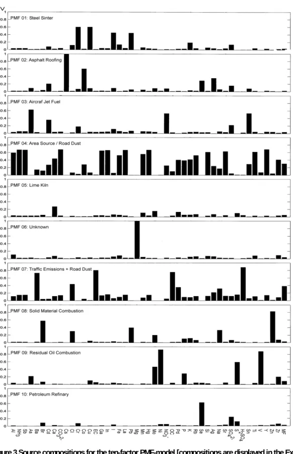
For example, the calculated factor PMF 01 contains high contributions of the elements chromium (Cr), copper (Cu), iodine (I) and lead (Pb). Based upon the comparison with the SPECIATE profiles, this profile matches reasonably well with the profile for a Steel Sinter. The first factor was therefore interpreted as emissions related to a Steel Sinter.

(28)

(29)

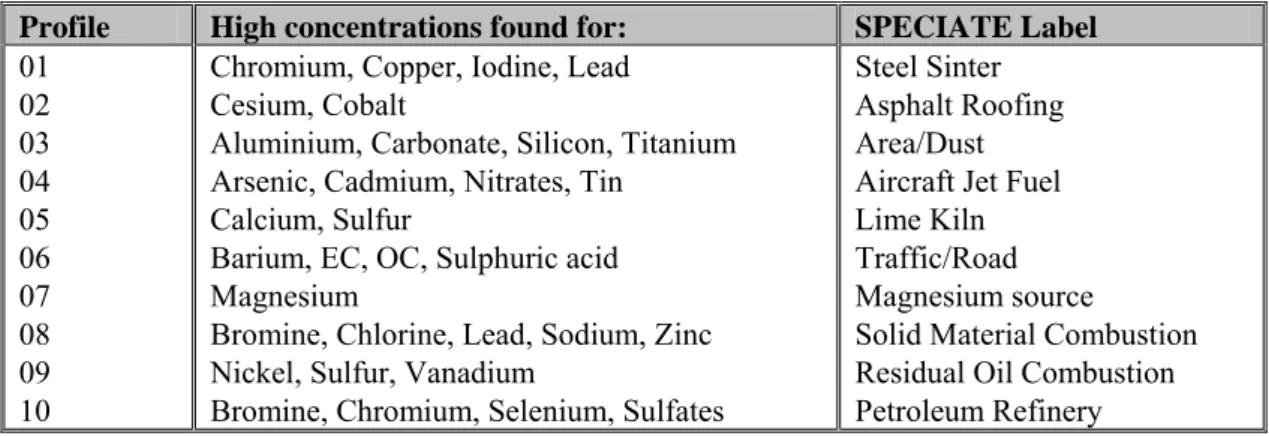
The identification process, which consists of comparing the elemental compositions of the calculated sources with the known SPECIATE profiles, is repeated for all calculated factors. An overview of the identifying species and the corresponding match from the SPECIATE profiles for each calculated PMF profile are presented in Table 2.

Table 2 Identification of the factors by elemental composition.

Profile High concentrations found for: SPECIATE Label 01 02 03 04 05 06 07 08 09 10

Chromium, Copper, Iodine, Lead Cesium, Cobalt

Aluminium, Carbonate, Silicon, Titanium Arsenic, Cadmium, Nitrates, Tin

Calcium, Sulfur

Barium, EC, OC, Sulphuric acid Magnesium

Bromine, Chlorine, Lead, Sodium, Zinc Nickel, Sulfur, Vanadium

Bromine, Chromium, Selenium, Sulfates

Steel Sinter Asphalt Roofing Area/Dust Aircraft Jet Fuel Lime Kiln Traffic/Road Magnesium source

Solid Material Combustion Residual Oil Combustion Petroleum Refinery

In addition to evaluating F, we also evaluated G. Since G contains the source compositions, a time-series plot can be constructed. Examples of these plots for the ten-factor solution are shown in the Appendices. These plots were not examined in detail to identify the unknown sources.

3.2.4 Assignment of source types using meteorological data

In combination with both the map of the area and the meteorological data, it is possible to more or less pinpoint the direction of the unknown sources. The directions of the sources have to correspond with both the location on the map and the identification based on the elemental composition, as discussed earlier. The assignment of source types using meteorological data were performed using a self-made analysis tool that is based upon the information provided in Section 2.3.2.

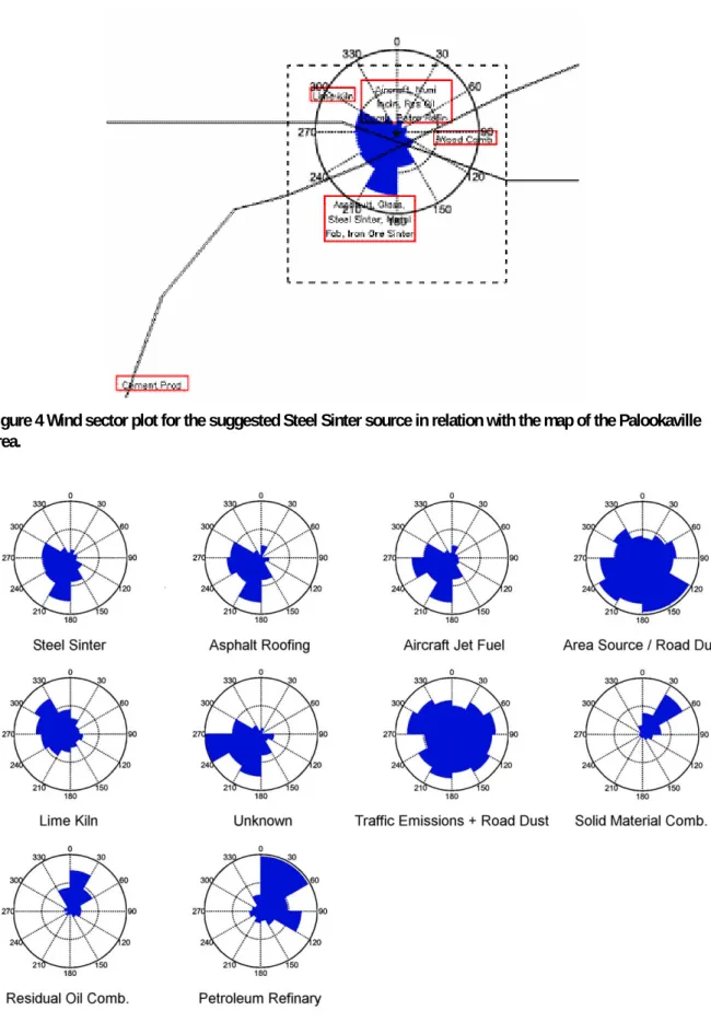
A wind sector plot containing the mass flux, as defined in Section 2.3.2 for the source labelled as a Steel Sinter, in combination with the map of the Palookaville area is shown in Figure 4. High mass fluxes represent the direction from which the highest source contributions originate. It can be seen that the highest mass flux is found between 180 and 210 degrees, which corresponds with the location of the Steel Sinter on the map.

Figure 5 shows detailed wind sector plots displaying the mass flux for each determined source profile as calculated by PMF. Each profile is named after the assignment based on the elemental composition. The wind sector plots containing the concentration values are given in Appendix 4. These plots also provide useful information, but application of the mass flux parameter was found to provide a clearer identification.

(30)

Figure 4 Wind sector plot for the suggested Steel Sinter source in relation with the map of the Palookaville area.

(31)

Other interesting profiles are those labelled Area Source/Road Dust and Traffic Emission + Road Dust. The wind sector plots do not provide a specific direction indicating where the source might be located; instead, the contributions from both sources seem to come uniformly from all directions. This

behaviour is typical of these kinds of profiles. As can be seen from the detailed map (Figure 2 or 4), the receptor point is enclosed by two major highways. It is expected the majority of the contribution of the Traffic Emission + Road Dust profile was contributed by these highways.

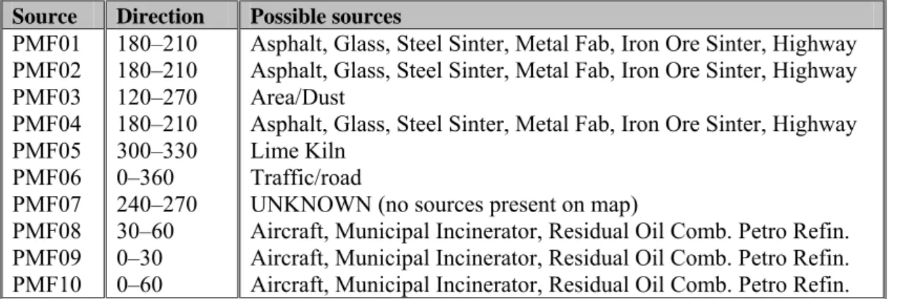
Table 3 provides the directions of the calculated sources profiles based on the wind-directional analysis and the sources present in these areas based upon the map.

Table 3 Source-specific directions for each factor compared with the location on the map. Source Direction Possible sources

PMF01 PMF02 PMF03 PMF04 PMF05 PMF06 PMF07 PMF08 PMF09 PMF10 180–210 180–210 120–270 180–210 300–330 0–360 240–270 30–60 0–30 0–60

Asphalt, Glass, Steel Sinter, Metal Fab, Iron Ore Sinter, Highway Asphalt, Glass, Steel Sinter, Metal Fab, Iron Ore Sinter, Highway Area/Dust

Asphalt, Glass, Steel Sinter, Metal Fab, Iron Ore Sinter, Highway Lime Kiln

Traffic/road

UNKNOWN (no sources present on map)

Aircraft, Municipal Incinerator, Residual Oil Comb. Petro Refin. Aircraft, Municipal Incinerator, Residual Oil Comb. Petro Refin. Aircraft, Municipal Incinerator, Residual Oil Comb. Petro Refin.

Most sources apportioned based upon the elemental compositions compare well with the directional behaviour found by the wind-directional analysis.

(32)

3.2.5 Differences between the assignments of source types

During our analysis, we found two major differences between the assignment based on elemental composition and the assignment based on meteorological data. Based upon the chemical composition data, the fourth factor was labelled as Aircraft Jet Fuel, but the direction of the fourth factor from the wind-directional analysis does not correspond to the location of the airport on the Palookaville map. On the map the airport is situated north of the receptor point, while the wind directional analysis places the airport between 180 and 210 degrees to the north. This anomaly was also reported by Henry (cited in Willis, 2000). Subsequent examination of the synthetic data set simulation by EPA-OAQPS revealed that the airport, the Asphalt Roofing manufacture and the Steel Sinter sources were in fact inadvertently located in the same place – approximately 200 degrees to the north (Willis, 2000). This claim

substantiates the location of the airport found by the wind-directional analysis in this study.

The second difference between the comparisons of both methods was discovered for the seventh factor. This source was labelled as an unknown magnesium source based upon the elemental composition. The wind-directional analysis places this source between 240 and 270 degrees, while the map provided with the dataset showed no sources in that direction.

At the Workshop on UNMIX and PMF as applied to PM2.5 it was revealed that the Palookaville dataset

contains an extra source (coal combustion) located to the southwest of the receptor. The presence of this source was deliberately withheld from the analysts (Willis, 2000).

Although the wind-directional analysis was able to determine the approximate location of this unknown source, it was not possible to make a correct identification based on the chemical composition data. Combining the results from the identification based on both the elemental composition and wind-directional analyses with the additional information presented at the Workshop (Willis, 2000), it was possible to identify the sources presented in Table 4.

Table 4 Identified sources for a 10-factor model. Source Label PMF01 PMF02 PMF03 PMF04 PMF05 PMF06 PMF07 PMF08 PMF09 PMF10 Steel Sinter Asphalt Roofing Area/Dust Aircraft Jet Fuel Lime Kiln Traffic/Road Magnesium Source

Solid Material Combustion Residual Oil Combustion Petroleum Refinery

(33)

3.2.6 Mass apportionment for the ten-factor solution

The predicted mass contributions from each source in G can be summed up to give the predicted total mass, and this latter value can then be compared with the measured mass, provided either the species which were not measured are strongly correlated to the measured species or they represent sources that add negligible mass to the PM samples.

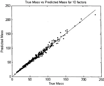
By making a simple plot of the predicted mass versus the measured mass and calculating the

correlation coefficient, we are able to determine whether the ten-factor model used in this case model accounts for the total PM mass. The correlation coefficient for this ten-factor model is 0.993, revealing that this model indeed accounts for the total PM mass. Figure 6 shows the predicted mass plotted against the measured mass. The line in the figure indicates the ideal function of Predicted = Measured. Through simple Ordinary Least Squares (OLS) regression it was determined that the equation of the line is Predicted = 1.20 + 0.983 × Measured.

When significant portions of the mass that are not directly correlated with the species in the PMF analysis are missing, it is possible to overestimate the source contributions using the regression with the mass values technique.

Figure 6 The relation between the measured (true) mass and the predicted mass from the contributions calculated by PMF. Also shown is the line corresponding to 1:1.

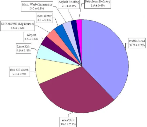
The average source contribution in the sampling period can be calculated from the predicted mass for each source. Figure 7 shows these average source contributions and the corresponding error estimates for the ten-factor solution.

Mass apportionment can also be applied directly from PMF by using the total mass for the daily samples as a variable – although with a very large error (i.e. low weight), such as fourfold the mass

(34)

value. In this case, the mass will not direct the fit but the portion correlated with the measured species will be apportioned.

Figure 7 Average source contributions for the sampling period, including the error estimates, by PMF for the Palookaville dataset.

(35)

3.3 Comparing the results with the known contributions

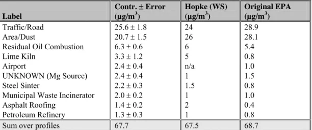
An overview of the average source contributions, the source contributions reported by Hopke (cited in Willis, 2000) and the source contributions used by EPA-OAQPS is given in Table 5.

Table 5 Overview of the average source contributions (in µg/m3_{) found in this study, those found by}

Hopke (cited in Willis, 2000) and those used by the EPA. Both Hopke and the EPA did not provide error estimates for the source contributions.

Label Contr. ± Error (µg/m3) Hopke (WS) (µg/m3) Original EPA (µg/m3) Traffic/Road Area/Dust

Residual Oil Combustion Lime Kiln

Airport

UNKNOWN (Mg Source) Steel Sinter

Municipal Waste Incinerator Asphalt Roofing Petroleum Refinery 25.6 ± 1.8 20.7 ± 1.5 6.3 ± 0.6 3.3 ± 1.2 2.4 ± 0.4 2.4 ± 0.4 2.2 ± 0.3 2.0 ± 0.2 1.4 ± 0.2 1.3 ± 0.3 24 26 6 5 n/a 1 1.5 1 2 1 28.9 28.1 5.4 0.8 1.0 1.5 0.8 1.0 0.4 0.8

Sum over profiles 67.7 67.5 68.7

The profiles in the table are classified on the basis of average contribution, which is expressed in micrograms per cubic metre (µg/m3). Traffic/Road and Area/Dust account for more than 65% of the total mass from this synthetic dataset.

A nine-factor solution was presented by Hopke at the Workshop on UNMIX and PMF as applied to PM2.5 (Willis, 2000), and we compared these results to those obtained using the ten-factor solution

(present study). The unknown magnesium source which we found (most likely to be the extra coal combustion source) is compared with an extra area source found by Hopke (cited in Willis, 2000). Hopke was unable to isolate the aircraft jet fuel profile in his runs with PMF.

Small differences between the calculated average contributions for each source in this study and the results of Hopke can be found. Detailed information provided by Hopke at the Workshop revealed a different approach to handling both the data points below the MDL and the corresponding error estimates: data points below the MDL were replaced by half of the MDL, and the uncertainties of these points were set to half the MDL (Willis, 2000). In general, this approach leads to a higher estimation of the standard deviation than was obtained in our study. The higher value of the standard deviation for data points below the MDL has the effect of making these points less important in the PMF analysis. Hopke also found that initial trials with PMF yielded low Q-values indicative of an incorrect weighting of the data. Alternative data weights were evaluated until the Q-value approached the theoretical value (Willis, 2000).

A comparison of the calculated average contributions with the original EPA data used in constructing the dataset revealed that the results obtained in the present study tend to overestimate the contributions

(36)

from the minor sources. PMF attempts to explain all of the observed mass with fewer profiles than used in the construction of the dataset, making an overestimation of smaller sources inevitable. The average contribution of the two larger sources, Traffic/Road and Area/Dust, were slightly underestimated, which suggests that at least some parts of the original profiles are similar to those of the smaller sources. Although enough information was extracted to identify the sources, the calculated profiles remain slightly mixed compared with their SPECIATE counterparts. An improved construction of the estimates for the standard deviation may reduce the effect of this problem.

3.4 Conclusion of the Palookaville exercise

In this study, data from simulated PM2.5 samples taken from the imaginary town of Palookaville were

analysed and compared to results obtained by Hopke (cited in Willis, 2000) as well as to the original contributions used to construct the dataset. After the analysis had been completed, all of the

information from the Workshop was disclosed. The basic assumptions in receptor modeling,

• Composition of source emissions are constant,

• Components do not react with each other (i.e. they add linearly), and • p (-identified or unknown) sources contribute to the receptor

will hold for the synthetic dataset used in this study.

A ten-factor solution was obtained from the data and compared to profiles from the SPECIATE database of known sources from the Palookaville area. Identified sources based on elemental composition include Steel Sinter, Asphalt Roofing, Area/Dust, Aircraft Jet Fuel, Lime Kiln, Traffic/Road, Solid Material Combustion, Residual Oil Combustion, Petroleum Refinery and a unknown magnesium source. The unknown source, containing only a high concentration of magnesium, could not be resolved on the basis of elemental compositions.

The results from the wind-directional analysis used in this study, in combination with the detailed map of the area, support the identification of all but two sources. One source, labelled Aircraft Jet Fuel was found in another location. Detailed analysis by the EPA–OAQPS revealed that the airport source was in fact not located at the position displayed on the map (Willis, 2000). The correct location corresponds well with the result from the wind-directional analysis.

The unknown magnesium source was placed southwest of the receptor site in an area without any known sources. However, the Palookaville dataset contains a ‘hidden’ extra source (Coal Combustion) located to the southwest of the receptor point. The location of this source was originally withheld from the analysts (Willis, 2000).

The three most dominant sources in the Palookaville dataset were extracted, and their average contributions to the total mass are quite comparable to results provided by Hopke as well as to the original contributions used to generate the dataset (Willis, 2000). The small difference between the results found in this study and those reported by Hopke can be mostly attributed to the different construction of the error matrix. Compared with the original EPA data, the results in this study tend to overestimate the contributions from the minor sources. This overestimation can be explained by the fact that PMF attempts to explain all of the observed mass with only ten sources; in contrast, 16 sources

(37)

Better estimates of the standard deviation used in the PMF analysis may reduce the effect of this problem.

Sufficient mass closure was found, with a correlation of 0.993 between the measured and predicted total mass for the ten-factor solution.

Using source-specific species from the profile, such as tracers, sources with small contributions (less than 5% of the average total mass) can still be determined. The wind-directional analysis is a valuable analytical tool for pinpointing directions in which the sources can be found. Together with a detailed map of the area containing sources, the wind-directional analysis can also be used for identification purposes. However, caution has to be exercised when examining sources with a small average contribution to the total mass because of the frequent overestimation of small sources by PMF.

(38)

(39)

4 Conclusion

Expertise in the field of receptor modeling was first gained from a number of literature studies and visits/discussions with experts working in this field. Detailed information on the steps necessary to perform source apportionment with Positive Matrix Factorization (PMF) is given in both Chapters 2 and 5. Based upon the literature studies, we developed a number of self-made analysis tools to facilitate our analysis of the results obtained with PMF.

The PMF model has been applied to a well-defined reference dataset that was provided by the US–EPA and which consists of simulated measurements in an imaginary town called ‘Palookaville’. The

analysis was performed without prior knowledge of the constituent source information. The result of the analysis, source profiles and time profiles together with some unusual discrepancies were reported to the US–EPA. At this point, the US–EPA sent back the complete description of the dataset together with the deliberately built-in discrepancies.

The sources that we found and the contributions of these sources to the reference dataset are in good agreement with the contributions used by the EPA to construct the dataset. The results are also compared to another study by Hopke (cited in Willis, 2000). The slight differences that are found in both the number of sources and the source contributions between these two studies are mostly attributable to different data pre-treatment.

During this study we have acquired sufficient confidence in both the Positive Matrix Factorization technique itself and in our level of experience. Both can now be applied to the analysis of real-life datasets.

(40)

Implementation of source apportionment using Positive Matrix Factorization - Application of the Palookaville exercise