Modelling emission of bio-aerosols carrying zoonotic microorganisms from livestock houses: quantification data and knowledge gaps

(1)

Thomas Hagenaars, José Gonzales, Clazien de Vos (Wageningen Bioveterinary Research) André Aarnink (Wageningen Livestock Research)

Report WBVR-1712754 May 2017

Modelling emission of bio-aerosols carrying zoonotic

microorganisms from livestock houses: quantification

data and knowledge gaps

(2)

Background and problem formulation

After the Q-Fever epidemic in The Netherlands, there is a growing interest in the potential risks zoonotic pathogens that may be emitted from farms pose to the health of nearby residents by air. Such pathogens may be viruses or bacteria. In order to carry out assessments of such risks for specific pathogens present on farms, it is often necessary to quantify the concentration of airborne viable pathogens that is emitted from a farm per unit of time.

For many viruses and bacteria it is very difficult to directly or reliably measure the concentrations of viable pathogens in the ventilation air. This difficulty arises because of low concentrations. For many microorganisms circulating in animals good information is available on concentrations in excreta, such as feces and (in diseased animals) urine. Therefore it is relevant to investigate whether concentrations of viable pathogens, emitted with the ventilation air, can be calculated from this information. To that end, a model could be developed that uses the information on excreted concentrations, information on the concentration of dust particles, their composition in terms of excreta and other materials in the house, and the rate of inactivation of the microorganisms before and during aerosolization. As part of this model development, the available knowledge on these processes has to be reviewed, more specifically: which measurement data are available for quantification of the processes, and what are the current knowledge gaps.

Based on the above reasoning the following study problems were identified:

a. Which quantitative data are available on concentrations of dust particles emitted with the ventilation air by different types of farms, and on the composition of those particles? b. Which quantitative data are available for relevant zoonotic pathogens on concentrations in

excreta and secreta and on inactivation during aerosolization?

c. Is it possible to reliably calculate the concentration of emitted viable airborne pathogens, based on characteristics of the type of animal production and type of housing system, based on the data reviewed in a and b, by using a mathematical model for the processes involved? If not, what are the knowledge gaps?

Approach

As shown in Chapter 6 of the main text, it is possible to perform informative air-sampling measurements on indicator organisms (E. Coli and Staphylococci) that are present in outgoing ventilation air of poultry and pig houses. This opens the possibility to investigate whether, for these specific organisms, a model could calculate the concentrations in ventilation air on the basis of underlying processes in a satisfactorily accurate way.

The following approach was chosen to study the problems a-c, as given above:

a. Based on a literature study and some new (unpublished) data, an overview was made of the available quantitative data on concentrations of aerosolized dust in the ventilation air and the composition of these aerosols for different types of animals houses. This overview took the form of an Excel database with quantitative data and references to the corresponding scientific publications.

b. Based on a literature study and some new (unpublished) data, an overview was made of the available quantitative data on pathogen concentrations in excreta and their inactivation rate when aerosolized, for a number of relevant zoonotic pathogens including avian influenza. Again, this overview took the form of an Excel database with quantitative data and references to the corresponding scientific publications.

c. A model (or model framework) was constructed for the calculation of emission concentrations of microorganisms based on the quantitative data gathered in parts a and b. By scrutinizing the overviews a and b from the structured perspective of the model we identified important knowledge gaps. The model was used to calculate/predict the concentration of the indicator organisms E. Coli and Staphylococci in outgoing ventilation air. A comparison of these predictions with measured concentrations was used to judge the current feasibility to make useful model predictions for emitted pathogen concentrations for the indicator organisms, and possibly for relevant zoonotic pathogens, and to articulate the most important knowledge gaps.

(4)

Materials and methods

Data collection

The data was collected from peer reviewed papers, field data generated by partners within the VGO project and grey data from field and experimental work carried out at WLR or WBVR. Data collection focussed on poultry and pig farms.

The following data types affecting emission of aerosols carrying microorganisms were included in the database:

1) Shedding: The shedding routes and corresponding concentration levels (measured e.g. in colony-forming units per gram feces (CFU/g) for bacteria and EID50/g for viruses) for the microorganisms of interest to the environment. The shedding routes are specific for the host-pathogen combination. As Illustrated in Fig 1, the route of shedding determines whether deposition on the floor is a necessary step before aerosolization may occur.

2) Survival: Survival rates of microorganisms during aerosolization; 3) Composition: Aerosol composition and particle-size characteristics;

4) Concentrations: Aerosolised dust concentrations (and emission rates) from livestock houses

Figure 1. Routes of shedding of pathogens and source of bio-aerosols: 1. Exhaled bio-aerosols (respiratory infections, e.g. influenza virus), 2. Bio-aerosols from exhaled or secreted (saliva) pathogens deposited on the floor (e.g. influenza virus), 3. aerosols from skin feathers (influenza virus), 4. Bio-aerosols generated from pathogens excreted via feces or urine.

An Excel database was created which contained different worksheets for the collection of information for the different data types listed above. The data collection for the data types 1 and 2 was mainly focussed on Escherichia coli (gram negative), Staphylococcus aureus (gram positive) and avian influenza virus (AIV). Data searches mainly but not exclusively targeted these microorganisms. When relevant information was limited for any of these microorganisms but available for other e.g. gram positive/negative bacteria, this information was recorded in the database. Further details on the four data types considered are as follows:

• Shedding. One dataset was created where information of the route of shedding and shedding concentrations for the reference pathogens was created. This dataset collected information on the host (species, production type, etc), the pathogen (species, serotype/type, etc), the route of excretion and level of shedding (mean, peak and length of shedding). Because there is an extensive body of literature on avian influenza, a comprehensive systematic review was performed to summarise data on shedding of this pathogen in poultry: A review protocol was built, consisting of an electronic search strategy, relevance screening, quality assessment and data collection. Studies describing virus shedding patterns of avian influenza in poultry were identified. The online databases of Pubmed, CAB Abstracts, AGRICOLA and Biological Abstracts were used to identify literature. A relevance screening was performed, followed by a quality assessment of the resulting citations, based on several criteria concerning experimental procedures. For example, inoculation route and sampling interval of virus shedding measurements must be described. Data was used to develop linear regression models predicting virus shedding levels for different combinations of avian influenza serotypes, poultry

(5)

species and shedding route. Parametric survival models were developed to quantify virus shedding length. For more details on the methods we refer to Sanders (2016).

• Survival. This dataset was created to collect information on survival of microorganisms in aerosol form. The focus of the review was on pathogen survival during the first stage of aerosolization (very short time, i.e. within the first minute of aerosol formation). Results on pathogen survival during the second stage of aerosolization (after the first minute) are given in the main text.

• Composition. A dataset was created where information on the sources of airborne dust were collated. The collected data describe the composition in terms of fraction of aerosolised dust originated from feces, bedding material, feathers/skin particles, urine, feed. Clearly, aerosol composition is dependent on factors such as the production system, type of housing, type of bedding/floor materials. Therefore these factors were taken into account in the data collection. • Emission. Here three datasets were created. These datasets were created to collate information

on (i) aerosol dust concentration in exhaust air of livestock houses, (ii) aerosol dust emission rates and (iii) concentration of indicator organisms in bio-aerosols in exhaust air of livestock houses. Also here the factors mentioned under “Composition” above will have an influence, and were therefore taken into account in the data collection.

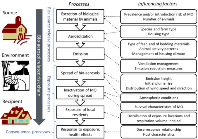
Modelling perspective

A standard structuring for assessment of health and environmental risks consists of partitioning the risk chain in three consecutive groups of processes: risk release processes, exposure processes and consequence processes. In Figure 2 we apply this partitioning to the zoonotic pathogen related health risk chain from livestock to local residents. Figure 2 distinguishes all risk release, exposure and consequence processes that may, to a certain level of detail, be considered relevant as building blocks of the risk chain. It presents a guiding line for the build-up of a modelling framework, representing and ordering the processes in the risk chain, and indicating relevant internal and external factors that influence the processes. In this report we are zooming into the risk release processes. We define “emission” as the concentration of viable microorganisms emitted by the farm (through time). We consider the emission process as a resultant of four risk release processes: excretion of biological material by the animals, aerosolization of dust containing such biological material (which results in bio-aerosols), transport of the bio-aerosols through ventilation to the air outflow of the farm, and (if present) a reduction of the outgoing bio-aerosol concentration though “end-of-pipe” reduction methods such as air filters.

The formulation of the specific models developed is based on the above process-oriented perspective in combination with considering the type of quantitative data on shedding, survival, dust composition and emission that is available to feed into a model. The desired output quantities of the modelling are:

• Number of microorganisms emitted per unit of time (= Emission level)

• Concentration of microorganisms in the exhaust air of the animal house. This quantity can be calculated from the emission level and the ventilation rate (for details see Results).

(6)

Figure 2. Flow diagram of an assessment framework for public health risks associated with zoonotic pathogen contained in bio-aerosols from livestock farming.

Results

Data overview

We first discuss the data overview for shedding and survival data of microorganisms, subsequently address the data available for dust composition, emission levels and concentrations in exhaust air, and finally present the data overview for the concentrations of indicator organisms in exhaust air. Whereas the first two data overviews are mainly composed of published data (published in the scientific literature), the last one consists of recent measurements that were carried out within the VGO research project and have therefore not yet been published up until the publication of this report.

(7)

Data overview: Shedding and survival

The literature data on shedding in feces of the enterobacteria E. Coli and Staphylococcus aureus in poultry and swine production systems contain both field and experimental data. As can be seen in the overview in Table 1, several field study results are available for fecal shedding of E. Coli in broilers. The mean or median shedding across different samplings (which may be either animal swab based, based on a pool of swabs, or pen-droppings based depending on the study) ranges between 6.4 and 7.5 log10 CFU/g, with minimum and maximum values of 4 and 8.4 logs, respectively. The observed variation between samples is thus quite large (a range of more than 4 logs). In the study by Horton et al. (2011) samples were collected from chicken cecal contents at 13 different abattoirs in the United Kingdom and it is not clear which part of the variation arises from differences between animals and which part from differences between flocks. However, in the study by Pleydell et al. (2007) the samples were collected from one single farm, and the variation in concentration is across a very similar range. Thus, when we are interested in the overall shedding level of many animals within one flock, the reported mean shedding levels of the studies ranging between 6.4 and 7.5 log10 CFU/g may be a good indication of the order of magnitude. The experimental study results by Van Bunnik et al. (2014) are in line with the field results. In the experimental study by Geidam et al. (2015) a pathogenic E. Coli strain was used, and a higher mean shedding (log10 10.8) was observed under these conditions.

For E. Coli shedding in layers, only one field study is listed in Table 1, with a mean shedding level of 6.5 log10 CFU/g, a value that is very similar to the observed means/medians for broilers. We note that since layer farms are emitting much more dust than broiler farms (see below for details), the layer farm type is one of prime interest for modelling the emission of pathogens. In this context, and given the fact that E. Coli is important for this modelling as an indicator organism, the availability of only one study on fecal shedding in layers, despite the similarity of its results to those of the studies in broilers, is a rather narrow basis.

In the context of pig farming, two field studies are available with results for E. Coli fecal shedding, both for fattening farms. The one published field study by Horton et al. (2011) observations ranged between 6.0 and 7.64 log10 CFU/g, whereas in the VGO study two feces samples taken in the stables (i.e. not directly from the animals) yielded concentrations close to 3 log10CFU/g. VGO study results on Staphylococci fecal shedding in fatteners, based on three fecal samples taken in the stables yield a mean concentration of 6.78 log10 CFU/g.

For avian influenza (AI) virus the literature on shedding in poultry is abundant. This all relates to small-scale infection or transmission experiments, which have been carried out for many different subtypes of highly pathogenic AI (HPAI) and Low Pathogenic AI (LPAI) viruses. As avian influenza is exotic to Dutch poultry, it occurs in poultry in an outbreak-wise fashion. This means that it is not being shed throughout the production period, as is the case for the indicator bacteria discussed above; furthermore the shedding level may change through the shedding period of an animal. For that reason we also extracted all information on the length of the shedding period and the peak shedding level from the literature. Using the systematic review approach with electronic search strategy, relevance screening and quality assessment, out of 2644 evaluated citations, 83 studies were used for data extraction. Chicken was the most commonly investigated species, while H5N1 was the most common serotype. A large heterogeneity existed in experimental methods used, including 14 different inoculation routes, 9 different sample sites and a range of different inoculation doses. A meta-analysis was performed on 47 studies reporting virus shedding levels as 50% egg infectious doses (EID50/ml), quantified by real-time polymerase chain reaction or virus isolation. This yielded a comprehensive summary of shedding patterns. The mean shedding level of HPAI (Table 2) is variable between studies with an overall mean close to 3 log10 EID50/ml; peak shedding is roughly 3.5 log10 on average EID50/ml. For LPAI the results of mean and peak shedding are very similar to HPAI (Table 3). Several factors including the virus subtype and the inoculation/infection method used influence the shedding pattern. These factors were identified by analysing shedding level using linear regression models and analysing shedding length using parametric survival models. For more details on the results we refer to Sanders (2016).

The published data on survival of various microorganisms is summarized in Tables 4 and 5. In Table 4 the data for microorganisms (including bacteria and viruses) are stratified by broad categories and in Table 5 these data are stratified by bacterial genus. All these data are from wet

(8)

aerosolization experiments, and relate to the survival in the first stage of aerosolization (<first minute). The distinction of two phases in the aerosolization is a very important aspect. In all these experimental data one can observe these two phases, with a comparatively strong inactivation within the first minute after spraying, and a less strong inactivation in a second, more stable, stage. Whereas the survival for the second stage observed in these experiments is thought to be most relevant for the pathogen survival during outdoor spread of the bio-aerosols emitted by livestock farms, the first stage is thought to be relevant to the process of aerosolization itself taking place when dust particles in livestock houses become airborne, and may be the dominant determinant of the total survival of microorganisms during aerosolization and the subsequent period of time that aerosols spend in the livestock house before being emitted. However, an important consideration here is that the latter process is a form of dry aerosolization, as opposed to the wet aerolisation technique used in the experiments. In Tables 4 and 5 we observe that humidity and temperature typically have a strong influence on survival during the first stage of (wet) aerosolization. Given the strong effects of humidity one may also expect substantial differences between the experimental results and the actual survival under (dry) field conditions. In addition, we observe large variation in survival rates estimated from different samples in the experiments. For example, as listed in Table 4, the observed survival percentage for E. Coli at 15-25 degrees Celsius temperature range and 40-70% humidity range varies between a minimum of 0.01% and a maximum of 86%, i.e. over three orders of magnitude.

Some insight into the potential difference in pathogen survival rates between wet and dry aerosolization conditions, may be obtained from dry and wet aerosolization experiments that have been performed for E. mundtii (Hoeksma et al. 2015). The results of these experiments are listed in Table 6, and suggest that for E. mundtii, the difference in survival between the wet and dry aerosolization conditions is very small. It should be noted, however, that the dry particles were prepared under lab conditions according the procedure as described by Hoeksma et al. (2015). The main treatment within this procedure was the freeze drying of the suspension of dust and bacteria solution. Furthermore, the survival rate may differ for other bacteria, such as gram-negative bacteria.

Table 1. Fecal shedding (log10 CFU/g) of viable indicator bacteria (determined by culture) in livestock.

Livestock Age (d) Bacteria Mean/median** SD Min Max n Type of data Ref

Poultry

layers 280 E. Coli 6.53 9 Field 1

broilers 28 E. Coli 6.5 12 Field 2

broilers 35 E. Coli 6.5 15 Field 3

broilers 46 E. Coli 7.54 4.90 9 32 Field 4

broilers 32 E. Coli 6.9 4 8.3 20 Field 5

broilers 59 E. Coli 6.4 5.1 8.2 20 Field 5

broilers 72 E. Coli 6.6 4.5 8.3 20 Field 5

broilers 14 E. Coli 7.3 0.94 5.63 7.48 9 Experimental 6

broilers* 10 E. Coli 10.77 10 Experimental 7

Pigs

fattening E. Coli 6.88 6 7.64 20 Field 4

fattening E. Coli 2.97 0.14 2.87 3.07 2 Field 8

fattening Staphylococci 6.78 0.71 5.96 7.27 3 Field 8

*This experiment used a pathogenic strain. **Median when Min/Max are given but SD is not given. Mean when no SD nor Min/Max are given or when SD is given.

References for Table 1:

1. Zhang ZF, Kim IH. Effects of probiotic supplementation in different energy and nutrient density diets on performance, egg quality, excreta microflora, excreta noxious gas emission, and serum cholesterol concentrations in laying hens. (2013). J Anim Sci. 91, 4781-7.

2. Cho JH, Kim IH. Effects of lactulose supplementation on performance, blood profiles, excreta microbial shedding of Lactobacillus and Escherichia coli, relative organ weight and excreta noxious gas contents in broilers. (2014). J Anim Physiol Anim Nutr (Berl). 98, 424-30.

(9)

3. Zhang ZF, Kim IH. Effects of multistrain probiotics on growth performance, apparent ileal nutrient

digestibility, blood characteristics, cecal microbial shedding, and excreta odor contents in broilers. (2014). Poult Sci. 93, 364-70.

4. Horton RA, Randall LP, Snary EL, Cockrem H, Lotz S, Wearing H, Duncan D, Rabie A, McLaren I, Watson E, La Ragione RM, Coldham NG. Fecal carriage and shedding density of CTX-M extended-spectrum {beta}-lactamase-producing escherichia coli in cattle, chickens, and pigs: implications for environmental contamination and food production. (2011). Appl Environ Microbiol. 77, 3715-9.

5. Pleydell EJ, Brown PE, Woodward MJ, Davies RH, French NP. Sources of variation in the ampicillin-resistant Escherichia coli concentration in the feces of organic broiler chickens. (2007). Appl Environ Microbiol. 73, 203-10.

6. Van Bunnik BAD, Ssematimba A, Hagenaars TJ, Nodelijk G, Haverkate MR, Bonten MJM, Hayden MK, Weinstein RA, Bootsma MCJ, De Jong MCM. (2014). Small distances can keep bacteria at bay for days. PNAS 111, 3556–3560.

7. Geidam YA, Ambali AG, Onyeyili PA, Tijjani MB, Gambo HI, Gulani IA. Antibacterial efficacy of ethyl acetate fraction of Psidium guajava leaf aqueous extract on experimental Escherichia coli (O78) infection in chickens. (2015). Vet World. 8, 358-62.

8. Unpublished data from the VGO research project.

Table 2. Highly pathogenic avian influenza virus shedding: Mean shedding, peak shedding and length of shedding. The units are EID50 per ml solution, and this in good approximation corresponds to EID50 per gram feces in case of fecal shedding. The data is a combination of virus isolation and qt-PCR results, as the results of these two methods were found to be highly similar.

Sample site Variable Level Mean shedding*

(95% CI) Peak shedding* (95% CI) Median length* (95% CI)

Cloacal Species Chicken 3,25 (2,05-4,45) 3,43(2,20-4,66) 1,21 (0,24-6,16)

Duck 2,70 (1,47-3,93) 2,88 (1,61-4,15) 4,05 (0,80-20,58) Goose 3,27 (1,27-5,27) 3,75 (1,67-5,83) 3,74 (0,73-19,02) Serotype H5N1 3,25 (2,05-4,45) 3,43(2,20-4,66) 1,21 (0,24-6,16) H5N8 2,52 (0,87-4,17) 3,02 (1,31-4,73) 1,21 (0,24-6,16) H7N3 2,18 (0,32-4,04) 2,93 (1,03-4,83) 1,21 (0,24-6,16) H7N7 1,65 (0,00-3,79) 2,23 (0,07-4,39) 1,21 (0,24-6,16)

Tracheal Species Chicken 4.26 (3.05-5.47) 4.48 (3.23-5.73)

Duck 3.71 (2.45-4.97) 3.93 (2.61-5.24) 4.97 (0.98-25.28) Goose 4.28 (2.26-6.29) 4.80 (2.70-6.90) 4.59 (0.90-23.35) Serotype H5N1 4.26 (3.05-5.47) 4.48 (3.23-5.73) 1.49 (0.29-7.56) H5N8 3.52 (1.86-5.19) 4.06 (2.33-5.79) 1.49 (0.29-7.56) H7N3 3.19 (1.31-5.07) 3.97 (2.05-5.90) 1.49 (0.29-7.56) H7N7 2.66 (0.52-4.80) 3.27 (1.12-5.43) 1.49 (0.29-7.56)

*Values are overall adjusted means. E.g. mean shedding for chickens is adjusted for virus serotype, inoculation route (not shown), age (not shown) and inoculation dose (not shown). Shedding values for each serotype are average expected values in poultry. These values were adjusted for poultry species, inoculation route, etc.

(10)

Table 3. Low pathogenic avian influenza virus shedding: Mean shedding, peak shedding (EID50/ml) and length of shedding (days). The data is a combination of virus isolation and qt-PCR results, as the results of these two methods were found to be highly similar.

Sample

site Variable Level Mean shedding* (95% CI) Peak shedding* (95% CI) Median length* (95% CI)

Cloacal Species Chicken 2.75 (1.64-3.83) 2.79 (1.71-3.87) 3.48 (1.45-8.34)

Duck 2.76 (1.64-3.88) 2.72 (1.56-3.88) 1.44 (0.60-3.45) Quail 3.03 (1.56-4.50) 4.10 (2.49-5.71) Turkey 3.01 (1.91-4.11) 3.19 (2.09-4.29) 2.56 (1.07-6.15) Serotype H5N1 4.08 (2.91-5.26) 4.18 (2.95-5.41) 3.40 (1.42-8.14) H5N2 2.75 (1.67-3.83) 2.79 (1.71-3.87) 3.48 (1.45-8.33) H5N3 2.61 (1.49-3.73) 2.62 (1.48-3.76) 2.18 (0.91-5.23) H7N1 2.61 (1.43-3.79) 2.74 (1.51-3.97) 4.04 (1.68-9.69) H7N2 2.04 (0.84-3.24) 2.36 (1.09-3.63) 9.73 (4.06-23.3) H7N7 3.56 (1.25-5.87) 4.79 (2.42-7.16) 4.83 (2.02-11.58) H7N9 3.05 (1.83-4.27) 3.28 (1.95-4.61) 9.28 (3.87-22.25) H9N2 2.75 (1.67-3.83) 4.02 (3.24-4.80) 6.86 (2.86-16.45) Inoculation route Contact 2.21 (1.11-3.31) 2.26 (1.03-3.50) Intrachoanal 2.41 (1.31-3.51) 2.52 (1.40-3.64) 2.39 (1.00-5.72) Intranasal (pooled) 2.75 (1.67-3.83) 2.79 (1.71-3.87) 3.48 (1.45-8.34)

Tracheal Species Chicken 3.09 (2.00-4.19) 3.17 (2.07-4.28) 4.16 (1.74-9.98)

Duck 3.11 (1.97-4.25) 3.11 (1.94-4.29) 1.72 (0.72-4.13) Quail 3.38 (1.90-4.86) 4.49 (2.86-6.12) Turkey 3.35 (5.25-4.46) 3.58 (2.45-4.71 3.07 (1.28-7.36) Serotype H5N1 4.43 (3.25-5.62) 4.57 (3.32-5.82) 4.07 (1.70-9.75) H5N2 3.09 (2.00-4.19) 3.17 (2.07-4.28) 4.16 (1.74-9.98) H5N3 2.96 (1.84-4.08) 3.01 (1.86-4.16) 2.62 (1.09-6.26) H7N1 2.96 (1.84-4.08) 3.12 (1.86-4.38) 4.83 (2.02-11.59) H7N2 2.39 (1.18-3.60) 2.74 (1.45-4.05) 11.65 (4.86-27.93) H7N7 3.90 (1.60-6.22) 5.17 (2.80-7.74) 5.78 (2.41-13.87) H7N9 3.40 (2.18-4.62) 3.67 (2.33-5.00) 11.11 (4.63-26.64) H9N2 3.94 (3.17-4.70) 4.41 (3.60-5.22) 8.22 (3.43-19.71) Inoculation route Contact 2.55 (1.51-3.60) 2.64 (1.53-3.76) Intrachoanal 2.76 (1.64-3.88) 2.91 (1.78-4.04) 2.86 (1.19-6.85) Intranasal _(pooled) 3.09 (2.00-4.19) 3.17 (2.07-4.28) 4.16 (1.74-9.98)

*Values are overall adjusted means. E.g. mean shedding for chickens is adjusted for virus serotype, inoculation route, age (not shown) and inoculation dose (not shown). Shedding values for each serotype are average expected values in poultry. These values were adjusted for poultry species, inoculation route, etc.

(11)

Table 4. Survival percentage of bacteria categories and viruses after the first

stage of aerosolization (within the first 1.0 min).

Pathogen temperature RH% Survival %

Median Min Max

Bacteria Gram negative (0,15] (0,40] 4.33 0 41.8 (0,15] (40,70] 9.75 0.02 38 (0,15] (70,100] 8.28 0.03 26.7 (15,25] (0,40] 4.7 0 79.1 (15,25] (40,70] 74.1 0.01 87.8 (15,25] (70,100] 46.8 0 81.1 (25,35] (0,40] 0.9 0 4.27 (25,35] (40,70] 0.24 0 6.5 (25,35] (70,100] 0.47 0 20.9 Gram positive (0,15] (0,40] 0.91 0.91 0.91 (0,15] (40,70] 0.01 0.01 0.01 (0,15] (70,100] 4.17 4.17 4.17 (15,25] (0,40] 0.54 0.54 0.54 (15,25] (40,70] 2.24 2.24 2.24 (15,25] (70,100] 6.5 0.7 51.29 (25,35] (0,40] 1.07 1.07 1.07 (25,35] (40,70] 14.45 14.45 14.45 (25,35] (70,100] 3.39 3.39 3.39 Virus Gumboro (0,15] (0,40] 6 6 6 Non enveloped (0,15] (40,70] 19.7 19.7 19.7 (15,25] (0,40] 2.2 2.2 2.2 (15,25] (40,70] 6 6 6 (25,35] (0,40] 0.1 0.1 0.1 (25,35] (40,70] 0.2 0.2 0.2 Influenza (15,25] (0,40] 1.7 1.7 1.7 Enveloped (15,25] (40,70] 15 3 19

(12)

Table 5. Survival of bacteria during the first stage of aerosolization (< first minute).

Genus temperature RH% Survival %

Median Min Max

Campylobacter (15,25] (70,100] 27.03 27.03 27.03 Chlamydia (15,25] (70,100] 15.9 15.9 15.9 Chlamydophila (0,15] (0,40] 25.1 8.4 41.8 (0,15] (40,70] 9.75 5.5 14 (0,15] (70,100] 21.6 16.5 26.7 (15,25] (0,40] 4.7 4.7 4.7 (15,25] (40,70] 8.2 8.2 8.2 (15,25] (70,100] 46 46 46 (25,35] (0,40] 0.9 0.9 0.9 (25,35] (40,70] 0.2 0.2 0.2 (25,35] (70,100] 20.9 20.9 20.9 Enterococcus (0,15] (0,40] 0.91 0.91 0.91 (0,15] (40,70] 0.01 0.01 0.01 (0,15] (70,100] 4.17 4.17 4.17 (15,25] (0,40] 0.54 0.54 0.54 (15,25] (40,70] 2.24 2.24 2.24 (15,25] (70,100] 31.8 12.3 51.29 (25,35] (0,40] 1.07 1.07 1.07 (25,35] (40,70] 14.45 14.45 14.45 (25,35] (70,100] 3.39 3.39 3.39 Escherichia (0,15] (0,40] 0.26 0.26 0.26 (0,15] (40,70] 34.2 1.82 38 (0,15] (70,100] 0.03 0.03 0.03 (15,25] (0,40] 1.45 1.45 1.45 (15,25] (40,70] 77.9 0.01 86.1 (15,25] (70,100] 62.5 0 63.73 (25,35] (0,40] 4.27 4.27 4.27 (25,35] (40,70] 3.25 0 6.5 (25,35] (70,100] 0 0 0 Klebsiella (15,25] (70,100] 46.8 46.8 46.8 Mycoplasma (0,15] (0,40] 0 0 0 (0,15] (40,70] 0.02 0.02 0.02 (0,15] (70,100] 0.05 0.05 0.05 (15,25] (0,40] 0 0 0 (15,25] (40,70] 3.63 3.63 3.63 (15,25] (70,100] 39.29 0.29 78.3 (25,35] (0,40] 0 0 0 (25,35] (40,70] 0.28 0.28 0.28 (25,35] (70,100] 0.47 0.47 0.47 Pasteurella (15,25] (0,40] 72.45 65.8 79.1 (15,25] (40,70] 78.3 78.3 78.3 (15,25] (70,100] 81.1 81.1 81.1 Pseudomona (15,25] (40,70] 74.1 64.4 87.8 Serratia (15,25] (70,100] 69.77 69.77 69.77 Streptococcus (15,25] (70,100] 0.7 0.7 0.7

(13)

Table 6. Survival of E. mundtii during the first stage of aerosolization from dry or wet aerosols. The main treatment within the experimental procedure for dry aerosolization was freeze drying of the suspension of dust and bacteria solution.

Media for

aerosolization Temperature RH% Survival %

Median Min Max

Dry 10 40 51.86 3.44 100 10 60 58.49 9.3 100 10 80 50.94 1.58 100 20 40 50.16 0.09 100 20 60 59.97 7.49 100 20 80 56.2 10.1 100 30 40 52.51 3.09 100 30 60 51.08 0.53 100 30 80 56.63 8.34 100 Wet 10 40 50.74 0.17 100 10 60 50.22 0 100 10 80 52.76 2.02 100 20 40 50.35 0.33 100 20 60 51.14 1.69 100 20 80 56.89 5.61 100 30 40 51.63 0.05 100 30 60 57.98 7.5 100 30 80 52.15 1.53 100

Data overview: Composition and concentrations

Fairly good information is available in the scientific literature on the composition of airborne dust in different farm types. This information is summarized in Table 7, distinguishing different production categories and housing types. The collected data describes the composition in terms of fraction of aerosolised dust originated from feces/manure, bedding materials, feed, feathers and/or skin, and “outside” dust, i.e. dust particles originating from outside the animal house.

Most of this information is originating from the study by Cambra-Lopez et al. (2011). There the data were interpreted using two alternative methods of analysis: classification rules and multiple linear regression. Although the overall correlation between the results of the two alternative models is good, for some specific farm types the percentage contributions of different sources may differ substantially (e.g. 13 vs. 72 percent manure contribution to PM2.5 dust in broilers on litter). This adds to the uncertainties in other parameters, although these uncertainties occur on a linear scale. For our modelling we used the results of the multiple regression method reported by Cambra-Lopez et al. (2011), because we are mainly interested in the quantitative contribution of each source to the airborne dust mass and not to the number of particles. In our opinion the method based on classification rules is very suitable for determining the contribution of each source to the number of particles, but less to estimate the contribution to mass, when compared with the multiple regression method. Given the logarithmic scale on which the concentrations and emission levels are expressed, the sensitivity to the uncertainties in composition of a model prediction for concentrations and emission levels is likely to be relatively minor.

Regarding dust concentrations (Tables 8 and 9) and, correspondingly, dust emission levels (Tables 10 and 11) information is available for a range of different production poultry and pig systems. In Table 11 we also include the available information for cattle and goats. An interesting comparison is that between caged layers and other types of layer housing: the caged production type, now forbidden in The Netherlands for animal welfare reasons, emits much less dust than the other types.

(14)

Table 7. Sources of dust in livestock houses determined within studies in NW Europe.

Type of livestock house _Size

fraction

Dust sources _Ref.;

Note

Category Housing Manure Bedding Feed Feathers/skin Outside

broilers litter PM2.5 13% 30% 14% 17% 25% 1; a

broilers litter PM2.5 72% 6% 0% 21% 1% 1; b

broilers litter PM10-2.5 47% 38% 2% 9% 3% 1; a

broilers litter PM10-2.5 96% 0% 0% 4% 0% 1; b

broilers litter inhalable >10% 0% <1% >10% 0% 2; c

layer aviary PM2.5 77% 0% 1% 22% 1% 1; a

layer aviary PM2.5 64% 0% 0% 36% 0% 1; b

layer aviary PM10-2.5 64% 0% 1% 32% 3% 1; a

layer aviary PM10-2.5 70% 0% 0% 30% 0% 1; b

layer cage inhalable 8% 0% 90% 12% 0% 3; d

layer perchery/floor PM2.5 26% 0% 3% 68% 4% 1; a

layer perchery/floor PM2.5 54% 0% 23% 17% 6% 1; b

layer perchery/floor PM10-2.5 57% 0% 4% 38% 1% 1; a

layer perchery/floor PM10-2.5 86% 0% 0% 15% 0% 1; b

layer perchery/floor inhalable 8% 68% 0% 12% 0% 3; d

fattening litter PM2.5 6% 28% 3% 30% 34% 1; a

fattening litter PM2.5 35% 26% 0% 39% 0% 1; b

fattening litter PM10-2.5 31% 14% 2% 49% 4% 1; a

fattening litter PM10-2.5 52% 23% 0% 25% 0% 1; b

dry/pregnant sows slatted PM2.5 14% 0% 36% 49% 1% 1; a

dry/pregnant sows slatted PM2.5 17% 0% 4% 79% 0% 1; b

dry/pregnant sows slatted PM10-2.5 41% 0% 3% 55% 2% 1; a

dry/pregnant sows slatted PM10-2.5 29% 0% 0% 71% 0% 1; b

fattening litter inhalable 24% 33% 5% 38% 0% 4; e

fattening slatted PM2.5 65% 0% 2% 29% 4% 1; a

fattening slatted PM2.5 93% 0% 1% 6% 1% 1; b

fattening slatted PM10-2.5 23% 0% 1% 68% 8% 1; a

fattening slatted PM10-2.5 30% 0% 1% 69% 0% 1; b

fattening slatted inhalable 30% 0% 30% 40% 0% 4; e

fattening slatted/litter inhalable 21% 28% 9% 42% 0% 4; e

rearing slatted PM2.5 62% 0% 4% 31% 3% 1; a

rearing slatted PM2.5 95% 0% 0% 0% 5% 1; b

rearing slatted PM10-2.5 31% 0% 6% 59% 4% 1; a

rearing slatted PM10-2.5 92% 0% 8% 0% 0% 1; b

rearing partially slatted inhalable 2-6% 0% >10% >10% 0% 2; f

a: using classification rules; b: using multiple linear regression; c: lower values & also >10% crystalline dust; d: upper values; e: mean values week 1, 4 and 7 after start fattening; f: lower values & also 1% crystalline dust.

References for Table 7:

1. Cambra-López M, Hermosilla T, Lai HT, Aarnink AJA, Ogink NWM. (2011). Particulate matter emitted from livestock houses: On-farm source identification and quantification. Transactions of the ASABE 54, 629-642. 2. Aarnink AJA, Roelofs PFMM, Ellen HH, Gunnink H. (1999). Dust sources in animal houses. In: Proceedings

of International Symposium on Dust Control in Animal Production Facilities, Aarhus, Denmark.

3. Muller W, and Wieser P. (1987). Dust and microbial emissions from animal production. In Strauch D (Ed.), Animal production and environmental health (pp. 47–89). Elsevier, Amsterdam, the Netherlands.

4. Aarnink AJA, Stockhofe-Zurwieden N, Wagemans MJM, 2004. Dust in different housing systems for growing-finishing pigs. In: Proceedings of Engineering the Future. AgEng 2004, Leuven, Belgium.

(15)

Table 8. Dust concentrations (mg/m3) in exhaust air of livestock houses determined within studies in NW Europe: poultry.

Type of livestock house Dust concentrations in mg/m3

Category Housing Country PM2.5 PM10 Respirable Inhalable Ref.

broiler litter Netherlands 1.05 10.36 1

broiler litter England 1.14 9.92 1

broiler litter Denmark 0.42 3.83 1

broiler litter Germany 0.63 4.49 1

broiler litter Netherlands 0.137 1.931 4.392 2

broiler litter Netherlands 7.44 6

broiler litter Netherlands 1.4—1.9 8.2—9 7

broiler breeder perchery Netherlands 0.12 1.703 2

chickens unknown Netherlands 0.48 3.88 1

layer aviary Netherlands 0.217 3.362 2

layer cage Netherlands 0.09 0.75 1

layer cage England 0.21 1.53 1

layer cage Denmark 0.23 1.64 1

layer cage Germany 0.97 1

layer perchery Netherlands 1.26 8.78 1

layer perchery England 0.35 2.19 1

layer perchery Denmark 0.92 4.86 1

layer perchery/aviary Netherlands 0.32 4.21 11

layer perchery/floor housing Netherlands 0.175 3.143 8.175 2

(16)

Table 9. Dust concentrations (mg/m3) in exhaust air of livestock houses determined in studies in NW Europe: pigs.

Type of livestock house Dust concentrations in mg/m3

Category Housing Country PM2.5 PM10 Respirable Inhalable Ref.

fattening pig litter England 0.15 1.38 1

fattening pig litter Denmark 0.1 1.21 1

fattening pig slats Netherlands 0.24 2.61 1

fattening pig slats England 0.29 2.67 1

fattening pig slats Denmark 0.16 2.08 1

fattening pig slats Germany 0.18 0.839 1

fattening pig litter Netherlands 0.16—0.71 2.08—5.67 12

fattening pig slatted Netherlands 0.23—0.34 2.14—2.94 12

fattening pig slatted/litter Netherlands 0.18—0.43 1.64—3.76 12

fattening pig slats/low-emission/dry feed Netherlands 0.0527 0.963 3.282 2

fattening pig slats/low-emission/wet feed Netherlands 0.0415 0.714 2

fattening pig slats/traditional Netherlands 0.0478 0.662 2.203 2

pregnant sow slats/group housing Netherlands 0.0378 0.415 2

pregnant sow slats/individual housing Netherlands 0.0535 0.485 1.245 2

Sow litter England 0.16 0.63 1

Sow litter Germany 0.12 1.64 1

Sow slats Netherlands 0.13 1.2 1

Sow slats England 0.09 0.86 1

Sow slats Denmark 0.46 3.49 1

Sow slats Germany 0.11 1.13 1

weaner fully slatted Netherlands 0.0511 1.091 2

weaner partially slatted Netherlands 0.0397 0.988 3.616 2

weaner slats Netherlands 0.32 3.74 1

(17)

Table 10. Dust emissions (mg/(h.animal)) in livestock houses determined within studies in NW Europe: poultry.

Type of livestock house Dust emissions in mg/(h.animal)

broiler litter England 1.69 14.8 1

broiler litter Denmark 0.99 7.5 1

broiler litter Germany 0.97 6.9 1

broiler breeder perchery Netherlands 0.43 5.8 2

layer cage Netherlands 0.18 1.6 1

layer cage England 0.68 3.7 1

layer cage Denmark 0.29 2.3 1

layer cage Germany 0.08 2.2 1

layer perchery Netherlands 2.60 16.5 1

layer perchery England 1.95 7.4 1

layer perchery Denmark 2.24 11.0 1

layer perchery Netherlands 0.57 10.6 28.3 2

layer perchery/aviary Netherlands 0.81 11.1 11

(18)

Table 11. Dust emissions (mg/(h.animal)) in livestock houses determined within studies in NW Europe: pigs, cattle and goats.

Type of livestock house Dust emissions in mg/(h.animal)

fatteners litter England 5.52 42.4 1

fatteners litter Denmark 7.25 93.5 1

fatteners slats Netherlands 7.42 77.5 1

fatteners slats England 9.49 63.9 1

fatteners slats Denmark 7.08 75.0 1

fatteners slats Germany 4.37 68.3 1

fattening pig slats/low-emission/dry feed Netherlands 1.02 23.8 96.8 2

fattening pig slats/low-emission/wet feed Netherlands 0.77 17.5 265.0 2

fattening pig slats/traditional Netherlands 0.83 16.4 53.0 2

pregnant sows slats/group housing Netherlands 1.41 19.8 2

pregnant sows slats/individual housing Netherlands 1.69 22.2 77.1 2

sow litter England 19.96 58.6 1

sow litter Germany 18.38 300.9 1

sow slats Netherlands 7.51 63.0 1

sow slats England 6.23 58.0 1

sow slats Denmark 60.51 796.5 1

sow slats Germany 5.09 43.4 1

weaner fully slatted Netherlands 0.26 7.6 2

weaner partially slatted Netherlands 0.24 9.5 34.2 2

weaner slats Netherlands 4.13 44.3 1

weaner slats England 1.49 17.1 1

weaner slats Denmark 1.50 40.0 1

weaner slats Germany 2.34 24.5 1

beef litter England 26.22 36.3 1

beef litter Germany 3.65 82.1 1

beef slats Netherlands 23.32 115.8 1

beef slats Denmark 3.22 50.3 1

beef slats Germany 6.53 109.1 1

calves litter England 7.11 16.3 1

calves litter Denmark 4.48 60.8 1

calves litter Germany 8.71 30.9 1

calves slats Netherlands 7.73 28.6 1

calves slats Germany 3.95 34.5 1

dairy cubicle Netherlands 1.65 8.5 2

dairy cubicle Netherlands 61.08 244.3 1

dairy cubicle England 21.38 24.9 1

dairy cubicle Denmark 15.22 134.6 1

dairy cubicle Germany 32.77 382.0 1

dairy litter Netherlands 14.23 65.7 1

dairy litter England 101.45 171.5 1

dairy litter Denmark 10.19 89.5 1

dairy litter Germany 6.91 87.6 1

(19)

References for Tables 8-11:

1. Takai H, Pedersen S, Johnsen JO, Metz JHM, Groot Koerkamp PWG, Uenk GH, Phillips VR, Holden MR, Sneath RW; Short JL, White RP, Hartung J, Seedorf J, Schröder M, Linkert KH, Wathes CM. (1998). Concentrations and Emissions of Airborne Dust in Livestock Buildings in Northern Europe. J. agric. Engng Res. 70, 59-77.

2. Winkel A, Mosquera Losada, J, Groot Koerkamp PWG, Ogink NWM, Aarnink AJA. (2015). Emissions of particulate matter from animal houses in the Netherlands. Atmospheric Environment, 111, 202-212. 3. Winkel A, Cambra-Lopez M, Groot Koerkamp PWG, Ogink NWM, Aarnink AJA. (2014). Abatement of

Particulate Matter Emission from Experimental Broiler Housings Using an Optimized Oil Spraying Method. Transactions of the ASABE / American Society of Agricultural and Biological Engineers, 57(6), 1853-1864. 4. van Harn J, Aarnink AJA, Mosquera J, van Riel JW, Ogink NWM. (2012). Effect of bedding material on dust

and ammonia emission from broiler houses. Transactions of the ASABE, 55(1), 219-226.

5. Aarnink AJA, van Harn J, van Hattum TG, Zhao Y, Ogink NWM. (2011). Dust Reduction in Broiler Houses by Spraying Rapeseed Oil. Transactions of the ASABE, 54(4), 1479-1489.

6. Aarnink AJA, Roelofs PFMM, Ellen HH, Gunnink H. (1999). Dust sources in animal houses. In: Proceedings of International Symposium on Dust Control in Animal Production Facilities, Aarhus, Denmark.

7. Ellen HH, Doleghs B, Zoons J. (1999). Influence of air humidity on dust concentration in broiler houses. In: Proceedings of International Symposium on Dust Control in Animal Production Facilities, Aarhus, Denmark. 8. Winkel A, Mosquera Losada J, Aarnink AJA, Groot Koerkamp PWG, Ogink NWM. (2015). Evaluation of a dry filter and an electrostatic precipitator for exhaust air cleaning at commercial non-cage laying hen houses. Biosystems Engineering, 129, 212-225.

9. Winkel A, Huis in 'T Veld JWH, Nijeboer GM, Ogink NWM. (2014). Maatregelen ter vermindering van fijnstofemissie uit de pluimveehouderij: validatie van een oliefilmsysteem op een leghennenbedrijf = Measures to reduce fine dust emission from poultry houses: validation of an oil spraying system on a layer farm. Wageningen UR Livestock Research.

10. Van Harn J, Ellen HH, van Emous RA, Mosquera Losada J, Nijeboer GM, Gerrits FA, Aarnink AJA, Ogink NWM. (2012). Maatregelen ter vermindering van fijnstofemissie uit de pluimveehouderij: effect van een waterfilm op het strooisel op de fijnstofemissie bij leghennen in volièresystemen = Measures to reduce fine dust emission from poultry: effect of water spraying on bedding material on the fine dust emission in aviary housing systems for layers. Wageningen UR Livestock Research.

11. Winkel A, Nijeboer GM, Huis in 'T Veld JW, Ogink NWM. (2013). Maatregelen ter vermindering van fijnstofemissie uit de pluimveehouderij: validatie van een ionisatiesysteem op leghennenbedrijven = Measures to reduce fine dust emission from poultry houses: validation of an ionisation system on layer farms. Wageningen UR Livestock Research.

12. Aarnink AJA, Stockhofe-Zurwieden N, Wagemans MJM. (2004). Dust in different housing systems for growing-finishing pigs. In: Proceedings of Engineering the Future. AgEng 2004, Leuven, Belgium. 13. Aarnink AJA, Mosquera J, Cambra López M, Roest HIJ, Hol JMG, Van der Hulst MC, Zhao Y, Huis in 't Veld

JWH, Gerrits FA, Ogink NWM. 2012. Emissies van stof en ziektekiemen uit melkgeitenstallen. Wageningen UR Livestock Research. Rapport 489.

Data overview: aerosolization factor

An interesting parameter that allows to compare the potential of different production system to bring fecal material into the air is the aerosolization factor. This factor is defined as the amount (in g) of dry matter dust (PM10) aerosolized per g feces. If assuming that the dry matter content of PM10 and of the feed are the same, the aerosolization factor can be calculated as the ratio of the amount (in g) of dust (PM10, dry + wet) aerosolized originating from feces and amount of feces excreted, e.g. both per animal. The amount (in g) of dust (PM10, dry + wet) aerosolized originating from feces can be calculated from the PM10 emission level and the PM10 composition. The amount of feces excreted can be calculated based on average feed intake per day per pig and the digestibility coefficient of dry matter in the feed. Calculations based on an average feed intake of 2.1 kg/d per growing-finishing pig and an average feed intake of 110 g/d per broiler indicate that the aerosolization factor of a broiler house is approximately six times as large as that of a house with fattening pigs. This is the net result of differences between these production types in terms of processes that promote the aerosolization of fecal material, such as drying out of feces and animal movement.

Concentration data for indicator organisms

In Table 12 we summarize the concentrations measured for the indicator organisms in the VGO samples of exhaust air in four different productions systems: pigs (sows & piglets), fattening pigs, sows, broilers and layers.

(20)

Table 12. Summary statistics for bio-aerosol concentration of indicator organisms (CFU/m3_{) in exhaust}

air of livestock houses, as measured in the VGO study and (if noted by a reference) in the literature.

Pathogen Production Culture (CFU/m

3₎ _{PCR (eCFU/m}3₎ n Mean Sd Mean Sd E. coli broilers 2,01 1,02 6,9 0,48 11 layers 1,55 0,97 _6,01 _0,27 ₂₃ pigs 0 0 ₀ ₀ ₃ fatteners 0 0 4,25 0,45 6 fatteners* 3,29 2.92 - 3.41 sows 0,34 0,63 4,75 0,8 6 Staphylococcus broilers 6,91 0,57 _8,44 _0,19 ₁₁ broilers# _{6,87 5.77 - 7.52} 4 layers 6,44 0,33 8,1 0,52 26 pigs 4,09 0,31 6,44 0,18 3 fatteners 3,6 0,4 6,09 0,39 6

fatteners and sows** 4,15 3.50 - 5.50 23

fatteners and sows (winter)## _{3,35 3.30 - 3.60} _{6,54 4.78 - 8.60 7 (11)}

fatteners and sows (summer)## _{2,51 2.00 - 3.23} _{5,63 4.77 - 7.67 5 (23)}

sows 4,88 0,45 6,26 0,39 6

*von Salviati et al. Veterinary Microbiology 175 (2015) 77–84. **Friese et al. Veterinary Microbiology 158 (2012) 129–135. #_{Friese et al. Applied and Environmental Microbiology 79 (2013) 2759–2766.}##_{Masclaux et al.} Ann Occup Hyg, 57 (2013) 550–557. Number of samples given in brackets are the samples PCR positive.

Modelling

Based on the above literature overview, we identify three types of data that could be used as a basis for a model calculation of inactivated + viable (i.e. PCR measured) microorganisms: data on shedding of microorganisms, data on dust emission/concentrations, and data on the composition of dust. Furthermore, data on survival of micro-organisms during aerosolization is available. A naive modelling approach based on working along the flow direction indicated in Figure 2, would be to explicitly describe the aerosolization process of dust (and microorganisms contained in the dust bio-aerosols) for each possible dust source, and calculate the overall dust bio-aerosol composition from there. However this requires much more quantitative insight in aerosolization rates of different materials under the specific conditions of the (type of) animal house in question than is available. Instead we note that the data available on dust composition allow us to directly work with the measured composition of dust that results from all the detailed aerosolization processes of the relevant different materials in the (type of) animal house considered. Furthermore, the measured PM10 dust concentration and emission data is a quantification of the absolute dust concentration and emission. Therefore we arrive at the following tentative modelling approach. We first consider the emission of inactivated + viable (i.e. PCR measured) microorganisms in PM10 dust bio-aerosols in the outgoing ventilation air. The level of such emission equals the PM10 emission level (in terms of PM10 mass per time unit) times the weighted average value for the inactivated + viable pathogen concentration in dust (in terms of pathogen units per mass unit), where the weighting is across dust sources and is performed using the percentage contributions of all the relevant materials that contribute to the dust, based on the available dust composition data. This model can be written in words and in mathematical terms as follows:

Emission Rate of Microorganism =

(PM10 Emission Rate) × SumOverDustComponents [PercentageContributionOfComponent* ConcentrationInComponent]

(

)

MO PM10

{manure,feathers,...}

i i i

ER

f c

i

=

∈

∑

(21)

Log((PM10 Emission Rate) × SumOverDustComponents [PercentageContributionOfComponent* ConcentrationInComponent])

(

)

MO

log

PM10

10 {manure,feathers,...}

i c i i

ER

f

i





=

_

_





∈

∑

Using the ventilation rate (VR) of the animal house we may convert the emission rate to a concentration (in terms of pathogen units per m3_):

Emission Concentration =

(Emission Rate) / (Ventilation Rate) MO

MO

ER

C

VR

=

When the emission concentration is measured in log units, the corresponding formula reads:

Emission Concentration =

Log ((Emission Rate) / (Ventilation Rate)) MO

MO

log

ER

C

VR





=

_

_





In order to calculate the emission (or concentration in exhaust air) of viable-only microorganisms, we need to account for the survival of the pathogen between shedding by the animals and emission of the dust bio-aerosols from the animal house. More precisely, the relevant survival for each particular dust source is the percentage of surviving pathogen between the moment at which the concentration shed (as in the shedding data overview) was determined, and the moment the exhaust air leaves the animal house. The model including the survival percentage reads as follows:

(PM10 Emission Rate) × SumOverDustComponents [PercentageContributionOfComponent* ConcentrationInComponent*SurvivingPercentageInComponent]

(

)

MO PM10

{manure,feathers,...}

i i i i

ER

f c s

i

=

∈

∑

Or when the concentrations in the components are measured in log units:

(PM10 Emission Rate) × SumOverDustComponents [PercentageContributionOfComponent* ConcentrationInComponent*SurvivingPercentageInComponent]

(

)

MO PM10

10 {manure,feathers,...}

i c i i i

ER

f

s

i

=

∈

∑

As argued in the data overview above, the most important part of the total inactivation between these two moments is taking place during the phase in which the material is drying out and small dusty particles are formed and/or the phase in which these particles are being aerosolized. Once the particles are air-borne for longer than roughly one minute, further inactivation typically occurs at a comparatively low rate. However, depending on the ventilation rate the second-stage inactivation may still make a relevant contribution in some cases. We will perform our scenario calculations ignoring this second stage, but consider the possible contribution of the second stage in the discussion of the comparison between model prediction and observations.

We note that the emission of a farm is time-dependent: its variability can be considerable (spikes and/or seasonal variability). This aspect is ignored by the above model, which is based on the emission data that may be viewed as time-average values. The aerosolization rates are influenced strongly by the level of animal activity, and thus variation in animal activity through time will cause time-dependencies in emission strength. In addition, the rate of aerosolization of dust is known to be influenced by the ventilation rate, which is known to vary through a production round and/or between seasons. The dust emission rate values of Tables 10 and 11 are based on a measured ventilation rate, concentrations in ingoing air and concentrations in outgoing air.

For microorganisms that are not always present on the farm, but only in periods of an outbreak, the stage of microorganism spread in the farm, for example measured by the number of animals infected, adds a factor that causes variation to other such factors present. In our explorative calculations below we assume that the emission scales with a within-herd prevalence P which is set to 1 for commensal bacteria, and to a fractional value for outbreak pathogens. This corresponds to changing the model equations to:

(22)

Prevalence × (PM10 Emission Rate) × SumOverDustComponents [PercentageContributionOfComponent* ConcentrationInComponent]

(

)

MO PM10

{manure,feathers,...}

i i i

ER

P

ER

f c

i

= ×

∈

∑

and similarly for the other equations above. The model input parameters and their units are summarized in Table 13.

Clearly the parameters P,

c

i and

s

i depend on the type of microorganism, whereas the parameters i

f

, ER, VR are related to the production system and housing system, and are independent of the type of microorganism. In order to account for the uncertainties in model parameters, stochastic model calculations (iterations) were performed in which model parameter values were sampled from probability distributions. Each iteration used a random assignment of model parameter values based on their joint probability distribution, and 10 000 iterations were performed to generate a distribution of outcomes, thereby providing insight into the uncertainty of the model prediction. These calculations were carried out using the @Risk software package. The probability distributions for the values of three production and housing-system related parameters used in our model calculations are listed in Table 14.

Table 13. Definition and notation of the model parameters.

Parameter Symbol Units

Within-herd prevalence P none

Concentration of microorganisms excreted in

excreta/secreta i e.g. feces

c

i log cfu/g (bacteria), log EID50/ml _(viruses)

Fraction of microorganism that survives during

aerosolization

s

i none

Fraction excreta/secreta i, in dust particles

i

f

none

Emission rate of dust particles (PM10) of the housing

system ER g/h/animal

Ventilation rate of the housing system VR m3/h/animal

Table 14. Input values for model parameters related to the production and housing system: Proportion of feces in dust particles ( f_F), emission rate (ER) (mg/h/animal), and ventilation rate (VR) (m3/h/animal).

Source: Cambra-López et al. 2011 ( f_F); Winkel et al. 2015 (ER and VR). The ER input values are based

on log-transformed data (Table 4 in Winkel et al. (2015)). Animal species Housing system

F

f

ER VR

Fattening pigs Part. slatted Normal(0.298,0.033)a _{eNormal(2.66,0.18)} _{Pert(6.6,28,49.3)}

Sows Group housing,

slatted floor 0.291 eNormal(2.9,0.27) Pert(22.2,50.8,75.9)

Layers Floor housing Normal(0.855,0.145)a _{eNormal(2.16,0.18)} _{Pert(1.1,3.5,9)}

Broilers Not specified Normal(0.956,0.017)a _{eNormal(0.81,0.18)} _{Pert(0.1,2.1,9.6)}

a_{Distribution bounded between 0 and 1.}

Model predictions for indicator organisms

We used the model to calculate/predict the concentration of the indicator organisms E. Coli and Staphylococci in outgoing ventilation air based on bacterial concentrations in feces. These feces were sampled in the same farms for which the concentration of bacteria was measured by sampling the exhaust air, thus enabling a comparison of the predictions to the measured concentrations. Such paired data were available for (fattening) pig farms (E. Coli and Staphylococci), and for two types of poultry farms (E. Coli only): layers and broilers. For these indicator bacteria, as they are commensurate bacteria, the within-herd prevalence parameter P was set to 1. The production and housing system related parameter distributions were those listed in Table 14. For both indicator bacteria, of the set of model parameters

f

_iwe only used

f

_F. For E. Coli we consider this to be a good approximation, assuming that the main dust source in which bacteria may be contained is feces. For Staphylococci it is not expected to be a good approximation, but rather a first step given a lack of quantitative data on concentrations in other dust sources, in particular nasal discharge and skin which are both expected to carry the bacteria.

(23)

Staphylococci in fattening pigs

Based on the VGO field data (see Table 1) the concentration of inactivated + viable Staphylococci in feces was modelled by a normal distribution with mean 6.78 log10 CFU/g and standard deviation of 0.71 log10 CFU/g. We assumed that in feces most of the bacteria are viable, and therefore used the VGO field data, which are based on culture of feces samples and thus measured viable Staphylococci only, as a measure for inactivated + viable.

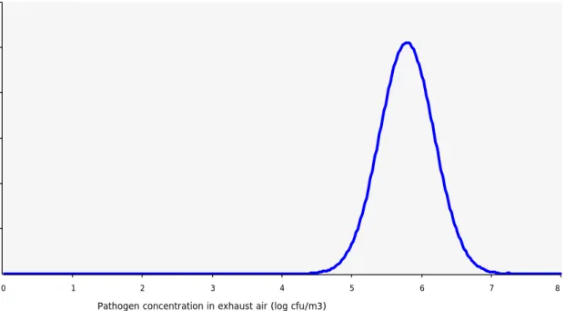
The model result for the concentration of inactivated + viable Staphylococci in exhaust air is given in red in Fig. 3. The variation indicated across more than 2 logs is due to the variation observed in measurements of the four underlying quantities: concentration of Staphylococci in feces, fraction feces in dust particles, emission rate and ventilation rate. In blue the measured concentration in PCR (i.e inactivated + viable) is displayed as a normal distribution based on mean and standard deviation calculated for the measurements (Here the PCR result for total dust was multiplied by 0.34 based on Mosquera et al. (2010) to convert it to a concentration based on PM10). The predicted mean concentration is approximately 2.5 logs lower than the measured concentration, which is a large discrepancy. This discrepancy, or part of it, could perhaps be explained by the contributions of skin and nasal discharge not being included in the model. Apart from that, replacing in the model the concentration in terms of CFU per gram feces by that in terms of CFU per gram dry matter in feces, would reduce the discrepancy by approximately 0.5 log. In addition, there are four input quantities that need to be considered in explaining the discrepancy: (possible inaccuracies in) the concentration shed in feces, the percentage of dust originating from feces, the emission rate and the ventilation rate. Inaccuracies in the latter two quantities are unlikely to contribute substantially to the observed discrepancy. The ratio of these is the dust concentration in the outgoing air, and the value for this ratio resulting from the literature values of the emission rate and the ventilation rate turns out to closely match the PM10 concentrations measured in parallel with the sampling for the indicator microorganisms. The quantity ‘percentage of dust originating from feces’ could also possibly only explain a small part of the discrepancy: the mean of this quantity is assumed to be 29,8% so that given a maximum of 100% the scope for underestimation is at most only 0.5 log. The concentration of Staphylococci shed in feces is an input quantity with much more scope for causing a large part of the discrepancy. If the value used (mean concentration of 6.78 log10 CFU/g) would be underestimating the true concentration in feces by 2 logs, that true concentration would need to be close to 9 logs. Clearly, further work would be needed to better understand how to reconcile measured concentrations in feces and in outgoing air. In addition, the predicted variation of the concentration is wider than the variation observed in the measurements. A plausible explanation for this would be that in samples of dust particles the contributions of feces of many different individual animals are included, such that much of the variation in concentration observed between individual fecal samples is averaged out.

(24)

Figure 3. Concentration of inactivated + viable Staphylococci in exhaust air of a house of fattening pigs: model prediction (red) and summary of measurements (blue).

Based on a survival fraction of 0.0224 for gram-positive bacteria in the first stage of aerosolization in the 15-25 degrees Celsius temperature range and the 40%-70% humidity range (taken from Table 4), we also used the model to predict the concentration of viable Staphylococci in the exhaust air. This was again based on assuming that the full bacteria concentration as determined in feces corresponded to viable bacteria. Here we observe a discrepancy between predicted and modelled concentration of close to 1.5 logs, with the model underestimating the measured viable bacteria concentration. Comparison of the measured viable Staphylococci in the exhaust air with the PCR results in Figure 3 indicates that the survival is roughly 1 log worse than described by the literature value of 0.0224 used. This is also more directly displayed in Table 15 in which the experimentally observed survival is compared to the one that may be deduced from the VGO culture versus PCR results on the same air samplings. As discussed above and apparent from Table 4, survival of gram-positive bacteria as measured experimentally is strongly dependent on the temperature and the humidity. This indicates that also in the field the survival in the first stage of aerosolization is rather sensitive to the precise conditions, and thereby also that differences between the experimental wet aerosolization conditions under which the results of Table 4 were obtained in the field can have a major effect on the survival. We note that in addition, second-stage inactivation (i.e. during the time the bio-aerosols spend in the house before being emitted) may explain part of the discrepancy of approximately 1 log.

0 1 2 3 4 5 6 7 8

Pathogen concentration in exhaust air (log cfu/m3)

0.0 0.2 0.4 0.6 0.8 1.0 1.2

(25)

Figure 4. Concentration of viable Staphylococci in exhaust air of a house of fattening pigs: model prediction (red) and measurements (blue).

Staphylococci in sows

The model results for the concentration of inactivated + viable Staphylococci in exhaust air of a sow house is given in red in Fig. 5. The concentration of inactivated + viable Staphylococci in feces was modelled again based on the VGO field data for fattening pigs, by a normal distribution with mean 6.78 log10 CFU/g and standard deviation of 0.71 log10 CFU/g. In blue the measured concentration in PCR (i.e. inactivated + viable) is displayed as a normal distribution based on mean and standard deviation calculated for the measurements. We observe a similar discrepancy between prediction and measured concentration to the one observed for Staphylococci in fattening pigs. Comparing the predicted and measured mean concentration shows that the model underestimates the mean by about 3 logs, which would be reduced to approximately 2.5 logs if correcting for dry matter content in feces as described above. Again this discrepancy, or part of it, could perhaps be explained by the contributions of skin and nasal discharge not being included in the model. If the contribution of feces would be dominant however, the only input quantity that could plausibly be responsible for most of the discrepancy is the concentration of Staphylococci in feces.

Based again on a survival fraction of 0.0224 for gram-positive bacteria in the first stage of aerosolization in the 15-25 degrees Celsius temperature range and the 40%-70% humidity range (taken from Table 4), we also used the model to predict the concentration of viable Staphylococci (see Figure 6). Comparison with Figure 5 shows that in this case the survival fraction of 0.0224 seems to give a better description of the observed survival than for fattening pigs. This is also more directly displayed in Table 15 in which the experimentally observed survival is compared to the one that may be deduced from the VGO culture versus PCR results on the same air samplings. The latter value is slightly higher, a difference which would increase after the contribution of second-stage inactivation (i.e. during the time the bio-aerosols spend in the house before being emitted) would be taken into account.

-2 -1 0 1 2 3 4 5 6

0.0 0.1 0.2 0.3 0.4 0.5 0.6 0.7 0.8 0.9 1.0

(26)

Figure 5. Concentration of inactivated + viable Staphylococci in exhaust air of a house of sows: model prediction (red) and measurements (blue).

Figure 6. Concentration of viable Staphylococci in exhaust air of a house of sows: model prediction (red) and measurements (blue).

E. Coli in pigs

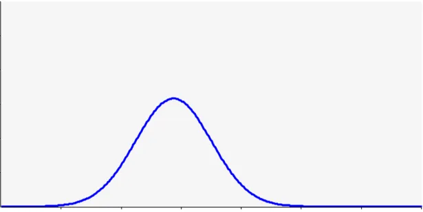
The concentration of E. Coli in feces was modelled by a Pert distribution with mean (min, max) 6.88 (6.0,7.64) log10 CFU/g based on the study by Horton et al. (2011) listed in Table 1. The model result for the concentration of inactivated + viable E. Coli in exhaust air is given in red in Fig. 7A (fattening pigs) and 7B (sows). The mean concentrations measured in the VGO field study are also displayed, and these were obtained by multiplying the PCR result for total dust by 0.34 based on Mosquera et al. (2010) to convert it to a concentration based on PM10. We again observe a large discrepancy between predicted and measured mean concentrations: 1 log for fatteners and 1.5 logs for sows. Again, replacing in the model the concentration in terms of CFU per gram feces by that in terms of CFU per gram dry matter in feces, would reduce the discrepancy by

0 1 2 3 4 5 6 7 8

0.0 0.2 0.4 0.6 0.8 1.0 1.2

Probability density function

-2 -1 0 1 2 3 4 5 6 7

0.0 0.1 0.2 0.3 0.4 0.5 0.6 0.7 0.8 0.9

(27)

approximately 0.5 log. Thus, the discrepancies are much smaller than in the calculations above for Staphylococci. However, we note that if the VGO field data for E. Coli in pig feces were used (see Table 1), the discrepancy would be even (almost) 4 logs larger. Regarding the variation in outcome, in contrast to what is observed for Staphylococci in pigs, the predicted variation in outcome is smaller than the one observed.

Based on a survival fraction modelled by Pert(0.0001,0.779,0.861) for E. Coli in the first stage of aerosolization in the 15-25 degrees Celsius temperature range and the 40%-70% humidity range (taken from Table 5), we also used the model to predict the concentration of viable E. Coli in the exhaust air. This was again based on assuming that the full bacteria concentration as determined in feces corresponded to viable bacteria. The result are shown in Figure 8A (fattening pigs) and 8B (sows). Comparison between Figures 7B and 8B shows that according to the measurements, the survival rate of E. Coli is much lower than suggested by the literature value. The difference for sows is 4 logs, as can be also seen in Table 15 where the rates are directly compared. For fattening pigs no viable E. Coli was measured in the outgoing ventilation air in the VGO field study (Table 10). This result is consistent with the fact that in experiments using dry aerosolisation, no viable E. Coli was recovered (Hoeksma et al. 2015).

Figure 7A. Concentration of inactivated + viable E. Coli in exhaust air of a house of fattening pigs: model prediction (red) and measurements (blue).

1.5 2.0 2.5 3.0 3.5 4.0 4.5 5.0 5.5 6.0

0.0 0.2 0.4 0.6 0.8 1.0 1.2

Modelling emission of bio-aerosols carrying zoonotic microorganisms from livestock houses: quantification data and knowledge gaps