A modular process risk model structure for quantitative microbiological risk assessment and its application in an exposure assessment of Bacillus cereus in a REPFED | RIVM

RIVM report 149106 007

A modular process risk model structure for quantitative microbiological risk assessment and its application in an exposure assessment of Bacillus cereus in a REPFED

M.J. Nauta

January 2001

This investigation has been performed by order and for the account of the Inspectorate for Health Protection and Veterinary Public Health, within the framework of project 149106, Quantitative safety aspect of pathogens in foods.

RIVM, P.O. Box 1, 3720 BA Bilthoven, telephone: 31 - 30 - 274 91 11; telefax: 31 - 30 - 274 29 71

in cooperation with F. Carlin, INRA, Avignon, France

Abstract

A modular process risk model (MPRM) methodology is presented as a tool for quantitative microbial risk assessment (QMRA). QMRA is increasingly popular to evaluate food safety and as a basis for risk management decisions. The MPRM provides a clear structure for transmission models of (complex) food pathways, that may involve the ‘farm to table’ trajectory. The MPRM methodology is illustrated in a case study, an exposure assessment of a sporeforming pathogen, Bacillus cereus, in a refrigerated processed food of extended durability (REPFED). This study is part of a European collaborative project. If contaminated with a psychrotrophic B. cereus strain, up to 6.5 % of the packages may contain more than the critical level of the pathogen at the moment the consumer takes the product from the fridge. This is, however, an uncertain estimate and its implications for public health are obscure. Some important gaps in knowledge are identified, for example the absence of growth and inactivation models that include variability, and useful quantitative models for sporulation, germination and spoilage. Also, the scarcity of data on consumer behavior concerning transport, storage and preparation is noted. Nevertheless, some risk mitigation strategies are suggested: decontamination of the ingredients that are added to the product, and improved temperature control of consumer fridge. Also, it is shown that a quality control at the end of industrial processing is highly insensitive. It was concluded that using MPRM is a promising approach, but that an improved interaction between risk assessment and microbiology is necessary.

Preface

This report describes research that is an integration of several projects. The methodology is part of the RIVM project 257851 ‘Exposure modelling of zoonotic agents in the animal production chain’. The exposure assessment is part of the project “Research on factors allowing a risk assessment of spore-forming bacteria in cooked chilled foods containing vegetables (RASP)”. The RASP project has been carried out with financial support from the Commission of the European Communities, Agriculture and Fisheries (FAIR) specific RTD programme, CT97-3159. It does not necessarily reflect its view and in no way anticipates the Commission’s future policy in this area, which at RIVM is classified under project 149106 ‘Quantitative safety aspect of pathogens in food’.

Many people have contributed to the work outlined here. First of all, the participants of the RASP project. Of those, Antonio Martinez, Pablo Fernandez, Auri Fernandez, Frederic Carlin, Roy Moezelaar, Sonia Litman and Gary Barker are acknowledged for their specific contributions to the work described in this report. Especially the many contributions of Frederic Carlin, co-author of chapter 3, were indispensable.

The description of the food pathway, and hence the whole study, was only possible by the availability of the production process, provided by a food manufacturing company, which is referred to as ‘company X’ throughout this report. This company is gratefully acknowledged. Due to both identified and unidentified uncertainties, the results in this report may in no way

be related to the quality of any of their products.

Several people at RIVM cooperated by their critical comments on (specific parts of) the research and earlier version of the report: Arie Havelaar, Eric Evers, Katsuhisa Takumi, Peter Teunis, Wout Slob and Frans van Leusden. They, too, are gratefully acknowledged.

Contents

1.3 The example: B. cereus in broccoli puree 15

1.3.1 The RASP project 15

1.3.2 B. cereus in broccoli puree 15

2. QMRA methodology : A modular process risk model (MPRM) structure 17

2.1 Setting up a QMRA 17

2.2 Setting up an MPRM 18

2.3 Modelling 19

2.3.1 Monte Carlo 19

2.3.2 Basic processes 22

3. Exposure assessment of Bacillus cereus in broccoli puree 35

3.1 Statement of purpose QMRA B. cereus in broccoli puree 35

3.2 The food pathway 35

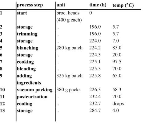
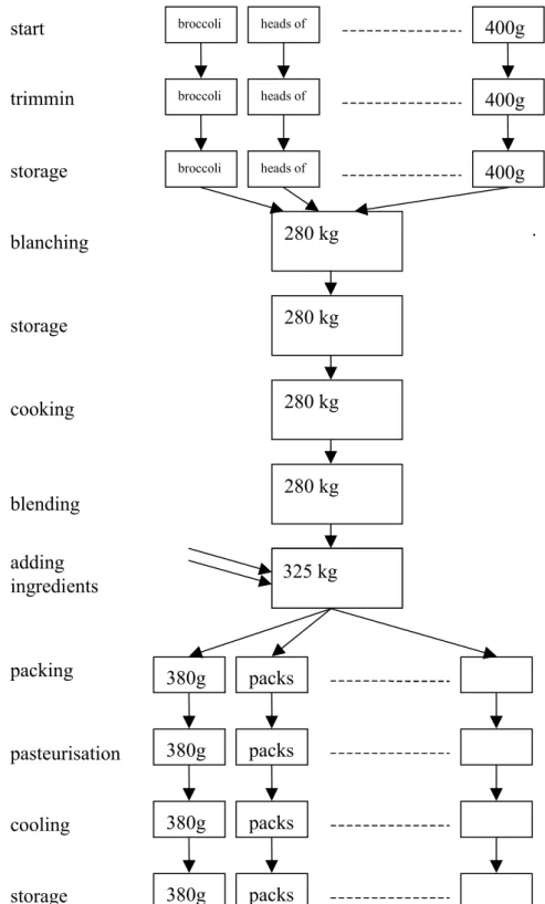
3.2.1 Industrial process description 36

3.2.2 Retailer and consumer handling 38

3.2.3 Identification of basic processes of the MPRM 40

3.3 Microbiological data 41

3.3.1 Raw material and initial contamination 41

3.3.2 Inactivation 42

3.3.3 Growth 43

3.3.4 Sporulation & Germination 45

3.3.5 Spoilage 45

3.4 The exposure assessment model 46

3.4.1 Modelling the Food pathway 46

3.4.2 Microbiology models and the implementation of microbiological data 53

3.4.3 The exposure assessment model 62

3.5 Results 65

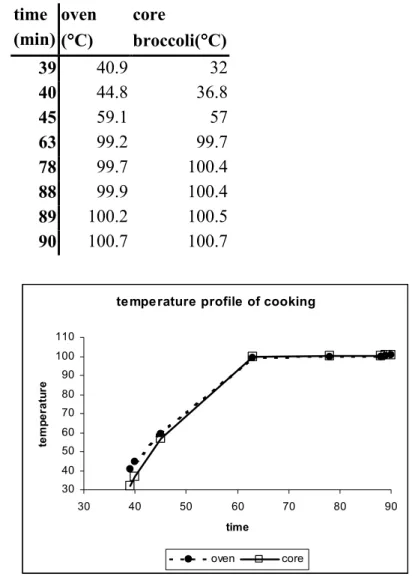
3.5.1 Detailed industrial model: The effect of cooking 65

3.5.2 Final model 66

3.6 Discussion 72

3.6.1 Results of the B cereus in broccoli puree exposure assessment 72

3.6.2 Microbiology and risk assessment 76

4. Evaluation of the MPRM 81

References 85

Appendix 1 Home refrigerator temperature distributions 91

Appendix 2 Output sheets 93

Samenvatting

Dit rapport combineert de methodologische beschrijving van een raamwerk voor kwantitatieve risicoschatting (QMRA) met een concreet voorbeeld, een blootstellings-schatting van Bacillus cereus in een groenteproduct. QMRA wordt in toenemende mate toegepast ten behoeve van de voedselveiligheid en ter ondersteuning van daaraan gerelateerd risicomanagement, zowel door voedselproducenten als door de overheid. Het kan een wetenschappelijke basis bieden voor de besluitvorming op het gebied van voedselveiligheid ten behoeve van volksgezondheidsbeleid en in de internationale handel. De methodiek van QMRA is nog volop in ontwikkeling. In dit rapport wordt voorgesteld voor de blootstellingsschatting een “Modular Process Risk Model” (MPRM) te gebruiken.

Het MPRM (Hoofdstuk 2) biedt een heldere structuur voor transmissiemodellen van complexe ‘voedselpaden’, die zich kunnen uitstrekken over het hele traject van boerderij tot tafel. Een ‘voedselpad’ is gedefiniëerd als de rij van processen van r(a)uwe producten tot aan consumptie door de mens en omvat zowel de industriële bereiding, de detailhandel als de consument. In het MPRM wordt aan elke processtap in het voedselpad in principe één specifiek basisproces toegewezen: groei, inactivatie, mengen, opdelen, verwijderen of kruisbesmetting. De transmissie van micro-organismen door het gehele voedselpad is vervolgens te modelleren door voor elk van de basisprocessen een apart transmissiemodel op te stellen. Als een processtap zo ingewikkeld is dat er geen basisproces aan is toe te wijzen of als belangrijke parameters onbekend zijn, kan een ‘black box’ model gebruikt worden.

Het MPRM biedt een heldere structuur, niet alleen door het opdelen in basisprocessen, maar ook doordat in de opzet zeven opeenvolgende stappen worden beschreven, die doorlopen moeten worden om een blootstellingschatting vorm te geven. Het wordt daardoor eenvoudiger de modelaannames expliciet te benoemen. In het MPRM worden zoveel mogelijk mechanistische modellen gebruikt. In principe hangt het opstellen van een MPRM daarom niet af van de beschikbaarheid van gegevens. Gegevens zijn “slechts” noodzakelijk om tot een betrouwbare risicoschatting te komen, niet om het MPRM op te stellen. Het gebruik van tweede orde Monte Carlo modellen, waarin onderscheid gemaakt wordt tussen onzekerheid en variabiliteit, wordt aangeraden.

De MPRM methodiek wordt middels een concreet voorbeeld van een blootstellingsschatting uit de doeken gedaan (Hoofdstuk 3). Het voorbeeld betreft een sporenvormende pathogeen,

Bacillus cereus, in een koelvers product, ofwel een “bewerkt, gekoeld levensmiddel met

verlengde houdbaarheid” (REPFED): een pak met gepureerde broccoli. Het bijbehorende onderzoek maakte deel uit van een Europees samenwerkingsverband in een project over sporenvormende bacteriën in voedsel, afgekort tot RASP. Aan dit EU-project namen onderzoeksinstituten en levensmiddelenproducenten uit verschillende landen in Europa deel. Uit de blootstellingsschatting kan geconcludeerd worden dat consumenten door consumptie van het onderzochte product blootgesteld kunnen worden aan B. cereus. De mate van blootstelling is in hoge mate afhankelijk van het gedrag van de consument. Met de huidige

kennis (die ondermeer inhoudt dat er geen dosis-respons relatie beschikbaar is), is het niet mogelijk het bijbehorende risico te kwantificeren, of met enige zekerheid een uitspraak te doen omtrent eventuele gezondheidsrisico’s die aan het onderzochte product verbonden zijn. Zoals opgemerkt, is van B. cereus geen dosis-respons relatie bekend. Op grond van epidemiologisch onderzoek wordt een concentratie van 105 cfu/g vaak als een kritische waarde beschouwd. Geschat wordt dat, op het moment dat de consument het product uit de koelkast haalt, 6.5% van de pakken een concentratie B. cereus van meer dan 105 cfu/g bevat. Het betreft dan een psychrotrofe stam. Deze schatting is echter erg onzeker, en de consequenties van dit resultaat voor de volksgezondheid zijn vooralsnog niet in te schatten. Het is echter wel mogelijk maatregelen aan te wijzen, die de blootstelling aan B. cereus kunnen verlagen en daarmee het potentiële risico kunnen reduceren. De belangrijkste zijn decontaminatie van enkele ingrediënten die tijdens het productieproces aan het product worden toegevoegd, en een verbeterde beheersing van de koelkasttemperatuur bij de consument thuis. Steekproefsgewijze controle van producten aan het einde van de industriële productie is weinig gevoelig, want besmetting daar is een slechte voorspeller van het uiteindelijke risico voor de consument.

Om blootstellingsschatting van sporenvormende pathogenen goed te kunnen uitvoeren is het nodig dat er groei- en inactivatiemodellen ontwikkeld worden, waarin ook variabiliteit wordt meegenomen. Ook is er grote behoefte aan wiskundige modellen die sporenvorming en ontkieming van sporen beschrijven. Vervolgens zijn er dosis-respons gegevens en modellen nodig om de blootstellingsschatting uit te breiden tot risicoschatting. Bovendien zijn er veel meer gegevens nodig omtrent consumentengedrag. Het gaat daarbij met name om kennis over de omstandigheden van vervoer, opslag en bereiding van levensmiddelen.

Er kan geconcludeerd worden dat het MPRM raamwerk veelbelovend is. Om QMRA uit te voeren is een verbeterende interactie tussen twee geheel verschillende vakgebieden, microbiologie en risicoschatting, onontbeerlijk. Het MPRM raamwerk zal hierbij in de toekomst behulpzaam kunnen zijn.

Summary

This report combines the methodological description of a framework for quantitative microbial risk assessment (QMRA) with a case study of Bacillus cereus in a vegetable product. QMRA is increasingly popular to evaluate food safety and as a basis for risk management decisions, both by food manufacturers and public health authorities. It may serve as a scientific basis for food safety issues for public health policy and in international trade. The methodology QMRA is however not well established. Therefore a Modular Process Risk Model (MPRM) methodology is presented here as a tool for exposure assessment.

The MPRM (chapter 2) provides a clear structure for transmission models of (complex) food pathways, that may involve the ‘farm to table’ trajectory. The food pathway is the line of processes from the raw product(s) until human consumption, that includes both the industrial processing and the retail and consumer handling. Essentially, in the MPRM each processing step in the food pathway is identified as one of six basic processes: growth, inactivation, mixing, partitioning, removal and cross contamination. The transmission of microorganisms through the food pathway can be modelled by formulating models of the transmission through each of these basic processes. If the transmission is too complex or if essential parameters are unknown, a ‘black box’ model may be used.

The MPRM has the advantage that is has a clear structure, not only by the identification of basic processes, but also by the proposing seven consecutive steps to perform an exposure assessment. This simplifies the explicit statement of the modelling assumptions. Next, MPRM uses mechanistic models as much as possible. In principle, constructing an MPRM does not depend on the availability of data. Data are ‘only’ relevant to come to a reliable risk estimate, using the MPRM, not for the modelling itself. The use of second order Monte Carlo models, separating uncertainty and variability, is promoted.

The MPRM methodology is illustrated in a case study, an exposure assessment of a sporeforming pathogen, Bacillus cereus, in a refrigerated processed food of extended durability (REPFED): a package of broccoli puree (Chapter 3). This study is part of a European collaborative project on sporeforming bacteria (abbreviated as RASP), involving research institutes and food companies throughout Europe. It was found that consumers may be exposed to B. cereus by consumption of the products. The level of exposure is highly influenced by the consumer behaviour. With the present knowledge (which is, among others, characterised by the lack of dose response information), it was not possible to quantify the risk, or to draw any ‘certain’ conclusions on the risk of the product.

At the moment there is no dose-response relationship available for B. cereus. Based on epidemiological studies, a concentration of 105 cfu/g is generally considered as a critical value. As an estimate, at the moment the consumer takes the product form the refrigerator there may be a probability up to 6.5% of dealing with a pack that contains more than 105 cfu/g, if contaminated with a psychrotrophic B. cereus strain. This is, however, an uncertain estimate and its implications for public health are obscure. Nevertheless, some promising risk

mitigation strategies can be identified, which will effectively lower the exposure to B. cereus. The most obvious ones are decontamination of some ingredients added during the production of the product and improved temperature control of consumer refrigerators. Controlling for food safety at the end of the industrial process by taking random samples there appears to be a bad predictor for food safety risk for the consumer.

It is concluded that exposure assessment of sporulating pathogens needs the development of growth and inactivation models that include variability and quantitative models for sporulation and germination. The development of dose response models is necessary to extend the exposure assessment to a risk assessment. Also, the scarcity of data on consumer behaviour concerning transport, storage and preparation is noted.

It was concluded that using MPRM is a promising approach, but that an improved interaction between risk assessment and microbiology is necessary. MPRM will be extendedly developed and applied in other QMRA’s in the near future.

1.

Introduction

1.1

Outline

Quantitative microbiological risk assessment (QMRA) modelling is increasingly used as a tool to evaluate food related health risks. Recently, an increasing number of papers has appeared that describe QMRA studies, for a range of micro-organisms and food products (Cassin et al. 1998a, Bemrah et al. 1998, Whiting and Buchanan 1997). However, as discussed below, the methodology of QMRA modelling is not yet established. Different approaches have been used so far, and several protocols and guidelines have been proposed. (CODEX Alimentarius Commission 1998, McNab 1998, Marks et al. 1998, Cassin et al. 1998a, ILSI 2000).

In this report we propose the use of modular process risk models (MPRMs) as a tool for risk assessment modelling. An important characteristic of this approach is the modular structure, that splits the food pathway into processing steps that describe one of six basic processes: growth, inactivation, partitioning, mixing, removal and cross contamination. In theory, once the modelling of these basic processes is established, any food pathway can be modelled when it is described as a sequence of consecutive basic processes.

The description of MPRM as a quantitative microbial risk assessment modelling framework is illustrated with an example: an exposure assessment of B. cereus in broccoli puree. The model constructed in this example is the result of a collaborative European research project on sporeforming pathogens in cooked and chilled vegetable products, abbreviated as ‘RASP’ (Carlin et al. 2000a).

The main objective of this report is to describe and illustrate a methodology, and examine its utility. With the example, we additionally identify some important gaps in knowledge and we are able to suggest some risk mitigation strategies for the specific product of concern.

1.2

QMRA methodology

The CODEX Alimentarius Commission (1998) guidelines for the conduct of microbial risk assessment gave a list of principles and definitions, but did not present a modelling methodology. McNab (1998) presented a framework for a Monte Carlo model of a generic food system. This framework describes the whole ‘farm to table’ pathway, and the additional health risks with biological and economical impact. However, it makes some disputable explicit choices for sub-models, and does not consider second order Monte Carlo modelling. As it has no modular structure, it is difficult to use as a general framework. Marks et al. (1998) used the term ‘Dynamical flow tree’ (DFT) modelling for their strategy. It incorporates the dynamics of microbial growth for microbial risk assessment. The DFT process is based on data and formal statistical inference or extrapolation from the available data. Cassin et al. (1998a) introduced the term process risk model (PRM) to describe the

integration and application of QRA methodology with scenario analysis and predictive microbiology. The emphasis of the PRM is to apply QRA as a tool that can be used to identify intervention procedures that might mitigate the risk, not the quantitative estimate of risk per se.

Van Gerwen et al. (2000) propose the use of stepwise quantitative risk assessment as a tool for characterisation of microbiological food safety. Their approach allows to tackle the main problems first, before focussing on less relevant topics. The first step is a broad, qualitative assessment, the second step a rough quantitative assessment and the third step a quantitative risk assessment using stochastic modelling. This approach is particularly useful in the development of food production processes and for pointing out crucial processing steps in the food pathway.

As a general framework, we propose a modular process risk model (MPRM) structure for quantitative microbial risk assessment. For a large part, it resembles the approach of Cassin et al. (1998a). Like their PRM, the model focuses on the transmission of the hazard along the food pathway, by describing the changes in the prevalence and the concentration over each of the processing steps. This food pathway includes production, processing, distribution, handling and consumption (Cassin et al. 1998b). With the model, the effects of ‘alternative scenario’s’, that is the effects of specified risk mitigation strategies or presumed changes in food processing or consumer behavior, can be assessed. However, our approach differs with that of Cassin et al. in two respects. First, it has a modular structure. It states that the transmission of the hazard through the food pathway can be regarded as a series of basic processes. The model structure is determined by this series of basic processes, as will be explained below. Unlike the DFT process (Marks et al. 1998) it is not based on the availability of data, but on knowledge of the food pathway processes. Second, we propose to use second order Monte Carlo modelling, that is the separation of uncertainty and variability in stochastic modelling. In this context, ‘uncertainty’ represents the lack of perfect knowledge of the parameter value, which may be reduced by further measurements. ‘Variability’, on the other hand, represents a true heterogeneity of the population that is a consequence of the physical system and irreducible by additional measurements (Murphy 1998, Anderson and Hattis 1999). Previously we have shown that neglecting the difference between these two may lead to improper quantitative risk estimates (Nauta 2000b). Without applying second order modelling dissimilar probability distributions are easily messed up, resulting in non-informative output distributions.

The MPRM may be used in any QMRA study, that is for industrial food processing and ‘farm to table’ risk assessment models. The focus is on modelling the food pathway and therefore on exposure assessment, that is the assessment of the dose of micro-organisms present in the food at the moment of consumption. Dose response modelling falls outside the scope of this report.

1.3

The example: B. cereus in broccoli puree

1.3.1 The RASP project

The example of the MPRM constructed in this report concerns B. cereus in broccoli puree packages. This example originates from a EU collaborative project entitled ‘Research on factors allowing a risk assessment of spore-forming pathogenic bacteria in cooked chilled foods containing vegetables (FAIR CT97-3159)’, abbreviated as ‘RASP’ (Carlin et al. 2000a). In this four year project (October 1996-September 2000) food microbiologists and risk assessors from INRA (France), IFR (UK), Nottingham University (UK), IATA (Spain), ATO (Netherlands) and RIVM (Netherlands) collaborated, with some food manufacturers from Spain, France and Italy, and SYNAFAP, a food processor association from France. As can be read from the project title, it concentrates on risk assessment of spore forming bacteria (SFB) in refrigerated processed foods of extended durability (abbreviated as REPFEDs), a new generation of cooked chilled foods. These REPFEDs follow the new consumer demands for more convenient, fresher, more natural foods of high organoleptic quality, which implies lighter preservation methods. REPFEDs are generally processed with mild heat-treatments and rely on refrigeration for preservation. Survival and outgrowth of SFB on REPFEDs may lead to food poisoning, and may therefore be an increasing threat to public health.

The project consisted of both experimental research and mathematical modelling on Bacillus

cereus and Clostridium botulinum from vegetable products. The concentration of experts

within the project allowed the construction some risk assessment models, using both the ‘Monte Carlo’-technique, and Bayesian networks. This report concentrates on the ‘B. cereus in broccoli puree’ MPRM, using the Monte Carlo technique. This example illustrates the use of most of the different modules as explained in the methodology section.

The RASP project has been structures around the guidelines as given in the Codex Alimentarius(1998). These guidelines state that a risk assessment should consist of a hazard identification, a hazard characterization (including a dose response assessment), an exposure assessment and risk characterization. As stated above, we concentrate on the exposure assessment. The results of RASP concerning the other parts of the risk assessment are discussed elsewhere (Carlin et al. 2000a, F. Carlin, G. Barker and others, unpublished).

1.3.2 B. cereus in broccoli puree

The choice for the hazard / product combination Bacillus cereus / broccoli puree is based on the results and expertise in the RASP project. With Clostridium botulinum, B. cereus is the ‘high risk’ hazard identified in the hazard identification (Van Leusden, unpublished). B.

cereus is a well known pathogen (e.g. Notermans and Batt 1998, Granum and Lund 1997,

Choma et al. 2000). An important characteristic, relevant for risk assessment, is that it is a sporeforming pathogen and may therefore be resistant to heat. The actual hazard is not the bacterial cell, but its toxin. B. cereus can form two types of toxin:

(1) an emetic toxin, which is preformed in the food, mainly found in rice products, and therefore not relevant in broccoli puree, and

(2) an enterotoxin, which is formed after outgrowth of the bacteria in the intestine and which is sensitive to heat and acidity. This is the toxin of interest in this study.

Unfortunately a dose response relationship, relating either toxin dose or pathogen dose to health effects, is unavailable. As discussed by Notermans et al. (1997), a level of 105 organisms per gram is generally considered as critical limit for acceptance of a food product. The absence of a dose respons relationship is the main reason that the risk assessment in the RASP project is restricted to an exposure assessment.

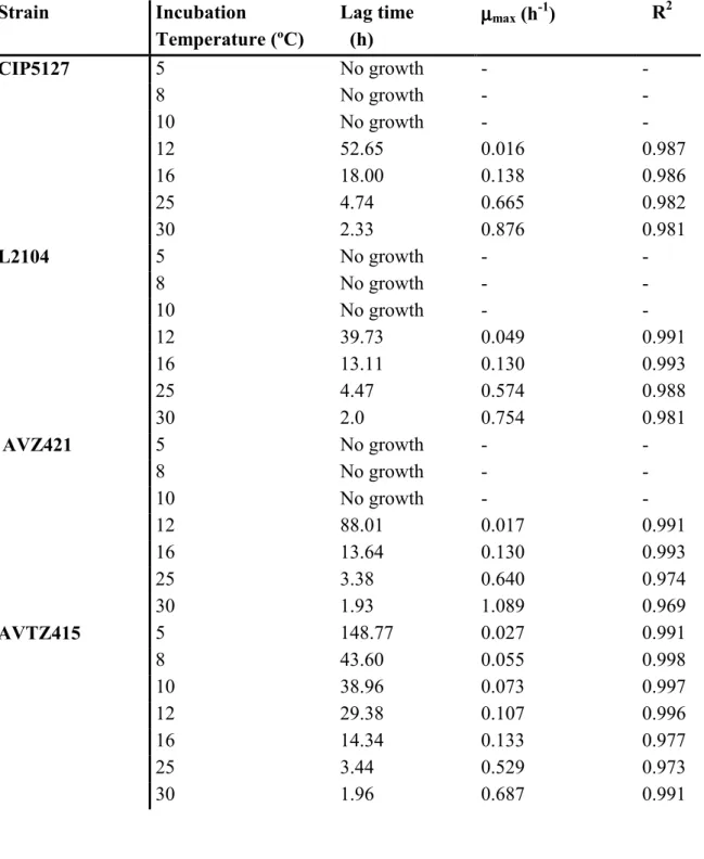
The variability in growth and inactivation characteristics between B. cereus strains may be large. A major type difference is that between psychrotrophic strains and mesophilic strains. The psychrotrophic strains are considered to be the major hazard in REPFEDs, as they are able to grow at low temperatures. However, mesophilic strains may be more heat resistant (Dufrenne et al. 1995), and might therefore be a hazard as a consequence of mild heating and severe temperature abuse.

The choice for broccoli puree as the product of interest is mainly based on the availability of data on its production process, some contamination data and some information on growth in broccoli broth.

2.

QMRA methodology : A modular process risk

model (MPRM) structure

2.1

Setting up a QMRA

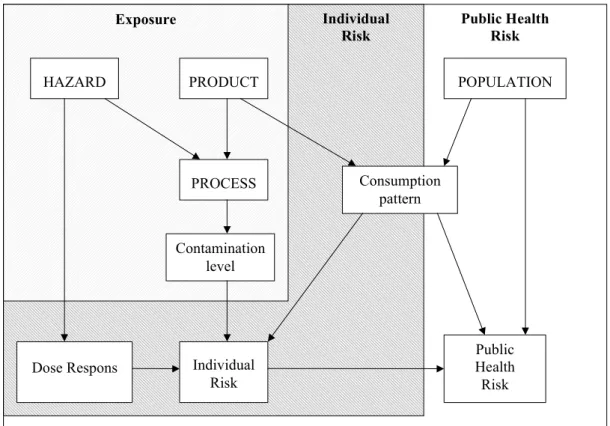
According to the CODEX Alimentarius Commission (1998) guidelines, risk analysis is the combination of risk management, risk assessment and risk communication. The aim of the risk assessment should be defined by the risk management. Next, the risk assessor needs several definitions before he can start the risk assessment. This is illustrated in Fig 2-1.

HAZARD Consumption pattern PROCESS POPULATION PRODUCT Contamination level

Dose Respons Individual

Risk

Public Health Risk

Exposure Individual

Risk Public HealthRisk

Figure 2-1 A risk assessment scheme. The boxes with capitals hold the items to be defined

before setting up the risk assessment. If risk assessment is restricted to either exposure assessment or assessment of individual risk, the scheme is reduced to the shaded areas. According to this scheme, exposure assessment is defined as the assessment of the level of contamination in a food product, independent of consumption patterns. Different assumptions or information on the consumption pattern is needed for assessment of individual risk and public health risk.

If the aim of the risk assessment is to assess a public health risk of consumption of a food product, definitions are needed of the hazard, the product, the population and the food pathway. Of these, the risk manager should at least provide the product and the population. It may be the task of the risk assessor to identify the hazard(s) and to define the food pathway, but these may also be part of the statement of purpose provided by the risk manager. In

microbiological risk assessment the hazard is the microorganism of concern (although the actual hazard may be a toxin it produces). The product is the food stuff consumed, and the food pathway is a description of the route of transmission of the hazard through the production process of the product until the moment of consumption. With these three a risk assessor should be able to assess the exposure, and, if a dose response relation is known, to assess the individual risk of consumption of the product. To assess the public health risk, one needs a definition of ‘public’, that is the population of concern. Consumption data of the product by that population are then needed to assess the consumption pattern. This has to be incorporated in the exposure assessment and combined with the dose response relation, to finalise the public health risk assessment.

As can be seen from Fig 2-1, definition of hazard, product and food pathway are necessary for exposure assessment. If the assessment has to be extended to some assessment of individual risk, one additionally needs a dose response relation, and if it has to be extended to assessment of the public health risk, one also needs a definition of the population.

If information on any of the requested items is lacking, it is possible to do a risk assessment, by making assumptions on e.g. the food pathway or consumption patterns of the population. It is important that these assumptions are clearly reported after finishing the risk assessment. Making assumptions should not be a problem in risk assessment, as long as they are explicitly reported, and as long as their impact is thoroughly discussed.

2.2

Setting up an MPRM

The modular process risk model (MPRM) is a tool for quantitative exposure assessment modelling. In general, the aim of the process model is to describe the transmission of the hazard along the food pathway, taking into account the variability and uncertainty attending this transmission. For this purpose, the food pathway is split up smaller steps, the modules. For each module, we are interested in the input-output relation for the number of cells per unit of product, N, and the fraction of contaminated units, the prevalence P. By treating both

N and P as uncertain and variable throughout the model, we will be able to assess the

uncertainty and variability in the final exposure, and thus the uncertainty in the final risk estimate.

Essentially, this input-output relationship can be obtained either by observation (direct in the production process (surveillance) or indirect in an experimental simulation (challenge testing)) or by mathematical modelling (see e.g. Notermans et al. 1998). The first method has the advantage that it is process-, product- and micro-organism specific, but the disadvantage that it is usually time consuming and expensive. The second method has the advantage that it is quick and cheap, but the disadvantage that it may be imprecise and not specific for the process studied.

Here we focus on the second method, mathematical modelling. We propose an approach for the exposure assessment in a QMRA which holds the following steps:

1) Define the statement of purpose, the (microbial) hazard and the food product. Consider which are the alternative scenario’s (either risk mitigation strategies, or potential changes is the process) that are to be evaluated with the model.

2) Give a description of the food pathway. Processing steps that involve potential alternative scenario’s may need a more detailed description than processing steps that will remain unchanged.

3) Build the MPRM model structure, by splitting up the food pathway into small processing steps (modules). In principle, each module refers to one of six basic processes, as explained in detail below. If a processing step is to complex or if essential parameters are unknown, and the processing step cannot be assigned to any of the basic processes, it can be considered as a ‘black box’ process.

4) Collect the available data and expert opinion, according to the model structure developed. 5) Select the model to use for each module, on the basis of the statement of purpose, process knowledge, data availability and the alternative scenario’s considered.

6) Implement the available data into the model. For each processing step, select the specific model to use. The use of mechanistic models is preferred, but only use complex models when this is necessary for evaluating alternative scenario’s and when the availability of data permits it.

7) Perform an exposure assessment.

2.3

Modelling

2.3.1 Monte Carlo

Monte Carlo simulation is a technique widely used in quantitative risk assessment. It allows working with stochastic models and to dealing with variability and uncertainty, whilst simulating the transmission of the hazard along the food pathway. Currently we use @Risk software for this purpose (Pallisade, Newfield, USA). @Risk can be used as an add-on to an Excel spreadsheet, and is therefore relatively easy to use.

A Monte Carlo simulation program runs a large number of iterations. In principle, each iteration represents one potential true event of transmission along the food pathway. A random (usually Latin Hypercube) sample is drawn from each of the probability distributions used as input for the model parameters. The model output is then again a probability distribution, that allows us to evaluate ‘probabilities’ of events, and therefore to evaluate risks. It is in all instances important to realise how an ‘event of transmission’ is defined and

what the input probability distributions represent. An ‘event of transmission’ may be the ‘one batch’ production of one food manufacturing site, the per day production of a particular food stuff in a region, or the yearly consumed quantity in a country. In principle all input distributions should depict probability distributions over the same ‘events of transmission’. If, for example, one distribution describes the variability per year and another the variability per day, these distributions cannot be mixed up without thorough consideration.

Monte Carlo simulation has the advantage that it widely applicable, comprehensible and relatively easy to use. Important disadvantages of the Monte Carlo method are that it needs precise probability distributions for all input parameters (see below), may require an enormous number of iterations in complex models, is difficult to use when modelling (non-linear) dependencies and may not be an adequate tool when rare events have a major effect on the final result. When performing a Monte Carlo in a spreadsheet, one occasionally has to use some approximations, to restrict the number of cells and to keep the model running. These approximations are sometimes inevitable, but always have to be handled with care.

2.3.1.1 Choosing a probability distribution.

Monte Carlo modelling needs a precise definition of the probability distributions of the input parameters. The choice of the ‘best’ probability distribution is not always straightforward. Criteria for choosing a distribution are usually natural characteristics of the parameter and the process modelled, or the quality of the fit of a distribution to data. Overviews of different probability distributions that can be used are widely available (Vose 1998, Vose 2000). The list below is restricted to a very short description of some frequently used distributions with their most important characteristics in the context of risk assessment and Monte Carlo modelling. This description is neither precise, nor complete.

2.3.1.1.1 Binomial

The binomial Bin(n,p) distribution describes the probability of x successes in n trials, when the probability of success is known to be p. It can be considered as ‘the mother of all probability distributions’. To be used when n is relatively small, and p nor 1-p is close to zero.

2.3.1.1.2 Poisson

The Poisson(λ) distribution describes the probability of x ‘rare’ events when the expected number of events is λ. The Poisson distribution is related to the Binomial by λ = np. The binomial distribution is approximated by Poisson when n is large (say n>50) and p is small (say np<5).

2.3.1.1.3 Normal

The Normal N(µ,σ) distribution is a continuous distribution characterised by the mean µ and standard deviation σ. The Normal distribution is related to the Binomial by µ = np and σ = √np(1-p). The binomial distribution is approximated by Normal when n is large (say np>

3√np(1-p)). The central limit theorem states that the sum of random variables with the same distribution approximately has a normal distribution. Many things in nature have a normal distribution. In many statistic tests it is assumed that the variables have a normal distribution.

2.3.1.1.4 Lognormal

In the lognormal distribution the logarithms of the parameter considered have a normal distribution. It has a lower limit zero, and a long tail. It is a convenient distribution because a log transformation allows one to treat multiplications as sums. It is important in (microbiological) risk assessment, because micro-organisms usually grow and die exponentially, and their numbers can therefore be considered as lognormally distributed. In general, many things in biology follow a lognormal distribution (Slob 1994).

2.3.1.1.5 Beta

The Beta(α,β) distribution is very flexible and well suited to describe the probability distribution of a probability, as it is bounded between 0 and 1. It can be used to express the uncertainty of the probability p in a binomial process when the number of successes s and the number of trials n is known. In that case, (assuming a uniform prior) p has a Beta(s+1, n-s+1) distribution.

2.3.1.1.6 Gamma (and exponential)

The Gamma(α,β) distribution is another continuous distribution with lower limit zero and no upper limit. It describes for example the probability distribution of the amount of time that lapses before α rare events happen, given a mean time between events β. If α = 1 (so if the time until a single event is of interest) the Gamma distribution is equal to the ‘exponential distribution’. An attractive characteristic of the Gamma distribution is that the sum of k random variables with a Gamma(α,β) distribution is Gamma (kα,β) distributed.

2.3.1.1.7 BetaPert

The BetaPert(min, mod, max) distribution (Vose 2000) is derived from the Beta distribution. It is well suited to describe the uncertainty of a parameter assessed by expert opinion. When the minimum, most likely and maximum value of a parameter are assessed the BetaPert can be used to represent its distribution. The same can be done with a Triangle(min, mod, max) distribution, but this has the disadvantage that it has a rigid shape with more weight in the tails.

2.3.1.2 Second order modelling: uncertainty and variability

As shown elsewhere (Nauta 2000b), separation of uncertainty and variability may be important in risk assessment modelling. ‘Uncertainty’ represents the lack of perfect knowledge of the parameter value, which may be reduced by further measurements. ‘Variability’, on the other hand, represents a true heterogeneity of the population that is a consequence of the physical system and irreducible by additional measurements (Murphy

1998, Anderson and Hattis 1999). At the moment, so called second order models (models that make the separation of the two) are scarcely produced in microbial risk assessment. The result is that the probability distributions of the final risk are a mixture of uncertainty and variability, and may give a wrong insight in the final risk.

The most important thing in this context is to make clear what the applied probability distributions describe. Variability can be variability in time, space, population(s), products etc. By explicitly identifying what the variability stands for, these things cannot be mixed up. A probability distribution describing variability can be uncertain, if the variability is not known exactly. Uncertainty can be very difficult to quantify. In that case the options are to neglect uncertainty and make qualitative statements on the uncertainty in the conclusions, or to assess the uncertainty throughout the risk assessment for all uncertain parameters by expert opinion or otherwise. To assess the uncertainty in the risk estimate, incorporating uncertainty for some uncertain parameters but neglecting it for others, is not a meaningful strategy. It may however be useful if the purpose is to assess the relative decrease in uncertainty of the final risk estimate by additional research on one specific risk factor.

2.3.2 Basic processes

The most important element of the MPRM approach is that we identify six basic processes, which are the backbone of every process risk model considered. These basic processes are the six fundamental events that may affect the transmission of any microbial hazard in any food process. There are two ‘microbial’ basic processes, growth and inactivation, and four ‘food handling’ processes, mixing and partitioning of the food matrix, removal of a part of the units, and cross contamination. The ‘microbial’ processes strongly depend on the characteristics of the microbial hazard, as the effects of environmental conditions on growth and inactivation differ per species (and even per strain). Essentially, the effects of the ‘food handling processes’ are determined by the food handling process characteristics only. Apart from aspects like ‘stickiness’ and cell clumping, which affect the distribution over the food matrix and may be different for different micro-organisms, they have the same effect on any hazard.

For each basic process a variety of models can be applied. The selected model for a certain module should be as simple as possible. Model selection will depend on the statement of purpose, process knowledge, data availability and the alternative scenario’s considered. If a process is well described, for example when process time, acidity and temperature are known, but microbiological data are scarce, one may use a predictive microbiology model to quantify growth or inactivation. If, on the other hand, data like microbiological counts before and after the process are available, but process parameters are not well known, it may be better to use a simple model relating the count data. If the process will remain unchanged, that if it is not part of any alternative scenario that changes the process, it is sufficient to have a simple description of the input-output relationship, without the involvement of any other parameters. (In that case it may, however, be necessary to use a complex model to derive this

relationship.) If, on the other hand, an alternative scenario changes the transmission of the hazard through the module, the effects of this scenario has to be part of the model.

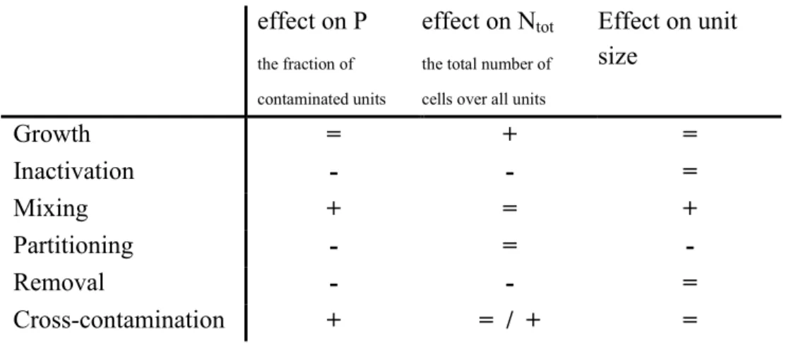
The qualitative impact on the transmission of each of these basic processes is given in Table 2-1. Note that the columns in this table do not depict the concentration, but the total number of organisms (N) and the ‘unit size’. The ‘unit’ is a physically separated quantity of product in the process, like for example a broccoli trunk, a carcass, a package of ground beef, a milk tank or a bottle of milk. The prevalence (P) in the table refers to the fraction of contaminated units. We prefer to use the number of organisms per unit and not concentrations. Doing so, we use only whole numbers in our calculations, which prevents the possibility of accidentally using ‘fractions of individual cells’. As a consequence of this approach, it is essential to precisely define the unit size.

Although it should be possible to allocate a basic process to each processing step in a food production process, this may either be difficult or unnecessary in practice. Therefore some (consecutive) processes are better regarded as ‘black boxes’. These processes may be very complicated and/or obscure. When there are no alternative scenario’s considered that directly affect such a process, detailed modelling is not necessary. In that case we propose a linear ‘black box’ model.

Table 2-1 Basic processes of the MPRM and their qualitative effect on the prevalence (P),

the number of organism in all units evaluated in one simulation run (Ntot) and the unit size. ‘=’ : no effect,; ‘+’: an increase; ‘-‘:a decrease.

effect on P

the fraction of contaminated units

effect on Ntot the total number of cells over all units

Effect on unit size Growth = + = Inactivation - - = Mixing + = + Partitioning - = -Removal - - = Cross-contamination + = / + =

How the transmission can be modelled quantitatively in each of the basic processes and with the ‘black box’ model is discussed below. The aim of the modelling of each of the basic processes is to describe the change in prevalence and number of micro-organisms per (contaminated) unit per processing step. The new prevalence (at the end of the basic process) is given by P’, and the new number or micro-organisms is given by N’. A change in unit size is usually defined in the food pathway description. P’ and N’ will be a function of N, P and the unit size, and possibly of some process parameters.

Note N and P, and possibly the unit size, are usually not fixed numbers, but stochastic variables that may be variable and uncertain. The prevalence P is a characteristic of all units at a step in the food pathway together. The number of micro-organisms N per unit may vary per unit.

2.3.2.1 Growth

The growth process is typical for microbial risk assessment. It is a variable, uncertain and complicating process. As can be seen from Table 2-1, growth gives an increase in both prevalence and number of micro-organisms and is therefore a particular risk increasing process. Due to growth, products that are contaminated at a low level and therefore are considered safe at a certain moment of time, may become unsafe later.

Growth is defined here as an increase in the number of cells N per unit. It does not affect the prevalence.

In general a growth model has the structure

log (Nout) = log (Nin) + f(.) (2.1)

with Nin the number of cells at the beginning of the process, Nout the number of cells at the

end of the process and f(.) an (increasing, positive) growth function. This growth function can have many shapes, which are widely discussed in literature (McMeekin et al. 1993, Whiting 1995, Baranyi and Roberts 1995, Van Gerwen and Zwietering 1998). For example, for exponential growth f(t) = µt (with t is time and µ is the specific growth rate), and when using the Gompertz equation f(t) = a exp[-exp(b-c t)], with parameters a, b and c.

As stated above, the selection of the ‘best’ model depends on of the statement of purpose, process knowledge and data availability. If, for example, a change in the temperature regime is considered, the model will need incorporation of ‘temperature’ as a parameter. Which specific ‘secondary growth model’ to select for this purpose, will depend on knowledge and the availability of data.

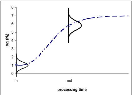
It is important to realise that a quantitative microbiological risk assessment growth prediction has usually different demands than a ‘traditional’ predictive food microbiology growth model prediction. Whereas the latter is used to come to a growth curve prediction, that is a series of point estimates of growth for a time series, in a risk assessment model, especially for a controlled food production process, one usually has to predict both variability and uncertainty in growth after a fixed time period (see Fig 2-2). Predictive microbiology models are not developed for this purpose, and therefore one has to be careful when applying them in a quantitative risk assessment study (Nauta 2000a, Nauta and Dufrenne 1999).

Figure 2-2 Growth is the increase in population size, given as log(Nt), as a function of time. Predictive microbiology models typically predict a growth curve, as given by the dashed line. In these models growth is considered as a function of time and the model yields a point estimate at any point of time t. In contrast, in QMRA we need a model that relates the probability distribution of the population size at the end of a process (out) to the probability distribution of the initial population size (in). Here, the end of the process may be at a fixed point in time. The probability distributions given by the ‘bell curves’ represent uncertainty and/or variability in population sizes Nin and Nout.

At the moment, to our knowledge, there are no predictive models available that are specifically designed to be used in a QMRA. Therefore, the best option is to use one of the available predictive microbiology models. Some of the frequently used models are response surface models based on data fitting, which are (commercially) available as computer software, like the Food MicroModel (Leatherhead Surrey, UK) and the Pathogen Modeling Program (PMP) (USDA, 1998). Another approach, primarily based on the principles of growth kinetics, allows a prediction if some of the growth characteristics (like the minimum and maximum temperature of growth) of the microorganism are known (Wijtzes et al. 1995, Zwietering et al. 1996).

It is not possible to say which model is the best choice in general. The PMP has the advantage that it is freely available at the internet and that it gives a confidence interval. It holds the problem that it is not clear whether this interval represents all of either variability or uncertainty or both. Also, the model prediction cannot easily be implemented in a risk assessment spreadsheet. Modelling according to the gamma concept (Wijtzes et al. 1995, Zwietering et al. 1996) has the advantage that it is a general model and can be easily applied to come to point estimates, but it gives no prediction of either uncertainty or variability. In general it can be stated that the important thing is not which model you use, but that you use it properly. If the QMRA includes uncertainty assessment, uncertainty and variability should be included in the growth prediction too. If the uncertainty and variability of the growth prediction are not known (which is usually the case), it is better to assess them by

0 1 2 3 4 5 6 7 8 processing time log ( Nt ) in out

expert opinion, then to neglect them, as this might result in an improper uncertainty interval around the final risk estimate. If different models are available which yield different predictions, this may be implemented as ‘model uncertainty’ into the model.

Although the variability in growth of micro-organisms will often be unclear, a method is available to predict the variability in growth, which is particularly relevant when the number of cells is low. This method addresses the variability of growth of a single strain and is derived from birth-process theory (Marks and Coleman, unpublished). It is shown that when there is a fixed probability over time that any cell will divide in two, the increase I in the number of cells N will have a negative binomial distribution with parameters s= N0 and p = e

-µt _and

E(I) = N0(eµt-1) (2.2)

var(I) = N0 eµt(eµt-1) (2.3)

Assuming exponential growth, E(Nt) = N0 eµt,it can be derived that

Nt ~N0 + Negbin(N0 , N0 /E(Nt)). (2.4)

Here we propose to use this equation as an approximation for the variability in growth for any growth model, so for any Nin = N0 and Nout = Nt.

As the negative binomial distribution approximates the normal distribution when the mean is larger than about 4 times the standard deviation, the normal distribution can be used when E(Nout )is large, that is when E(Nout)>Nin2/(Nin-16):

Nout ~ Normal(E(Nout), √ (E(Nout)(E(Nout)-Nin)/Nin)). (2.5) It may be necessary to use this approximation for large values of N in a spreadsheet program.

2.3.2.2 Inactivation

Microbial inactivation is the opposite of microbial growth. It is characterised by a decrease in the number of organisms per unit N. If the inactivation results in a decrease to zero living cells, the prevalence will decrease too.

The general formula for modelling inactivation is similar to equation (2.1)

log (Nout) = log (Nin)- g(.) (2.6)

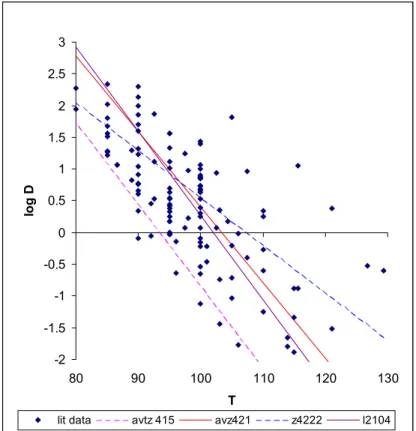
with g(.) an increasing (!) inactivation function. As for growth, many inactivation models are available (e.g.Van Gerwen and Zwietering 1998, Xiong et al. 1999). The most frequently used inactivation process is heating and the most frequently used inactivation model is the Bigelow model, in which inactivation rate is a function of temperature. It is linear in time (t)

and has the shape g(t) = t/D, when the D-value (the decimal reduction value) at the process conditions is known. When Dref , the D-value at temperature Tref, and the z-value are known, the same inactivation function holds at temperature T with

log(DT) = (T-Tref)/z + log(Dref ) (2.7)

Many of the aspects discussed for growth also apply for inactivation. Inactivation models are not developed to predict the uncertainty and variability around the final estimate. Confidence intervals may be derived from experimental data, but it is not straightforward whether to interpret this as uncertainty or variability. As for growth, an important aspect here is the differences that may exist between strains of a species, and even differences within a strain, due to adaptation (Nauta and Dufrenne 1999).

As for growth, the variability in inactivation can be predicted when the number of cells is low. If the probability of survival of a single cell during time span t is

p = e-λt = E(Nt)/N0 (2.8)

the number of survivors is

Nt ~ Binomial(N0,E(Nt)/ N0) (2.9)

distributed. This can be used as an approximation for the variability in inactivation for any

Nin = N0 and Nout = Nt. Note that when Nin is large (say Nin > 16 E(Nout )/(16-E(Nout))) this distribution is approximated by the normal distribution

Nout ~ Normal(E(Nout), √ (E(Nout)(Nin-E(Nout))/Nin)). (2.10) In contrast to the growth process, inactivation can result in a decrease in the prevalence. Once the number of cells in/on a unit drops to zero, the prevalence will decrease. The probability of this happening in a unit can be derived from the equation above as (1-E(Nout)/Nin)Nin which ≈ e-E(Nout) when E(Nout)/Nin is small. Hence the predicted prevalence after inactivation, if all units are equal, is

Pout = Pin(1-(1-E(Nout)/Nin)Nin). (2.11)

2.3.2.3 Partitioning

Partitioning affects the food matrix. It occurs when a major unit is split up into several minor units, as given schematically in Fig 2-3.

unit with N cfu

x units i=1 i=2. ... i=x

Figure 2-3 Partitioning: A major unit, containing N cfu (particles, spores, cells, etc) is split

up in x smaller units i (i= 1..x). The problems to be solved are: (1) what is the number of smaller units with zero cfu and (2) what is the distribution of Ni, the numbers of cfu over the x minor units that are contaminated ?

With the model we have to describe the distribution of the N cells in the major unit over the x smaller units.

First, consider a possible change in prevalence. If, due to sampling effects, any of the smaller units contains zero cells, the prevalence will decrease. Assuming random sampling, the probability of an ‘empty’ smaller unit, P(zero cells in smaller unit) = P(0) = (1-1/x)N, so the new prevalence

P’=P×(1-(1-1/x)N_{). (2.12)}

The expected number of empty smaller units is then

E(x0) = x.P(0) = x1-N(x-1)N. (2.13)

Due to the interdependence between the numbers in the smaller units, we were not able to derive the standard deviation in x0 analytically. It is smaller than expected from a binomial expectation:

σ(x0) < √(x P(0)(1-P(0)) =√(x1-N(x-1)N - x1-2N(x-1)2N) (2.14) If P(0) is small (that if is N is large and x is relatively small), x0 can be assumed to have a Poisson(E(x0)) distribution. Then, the number of empty smaller units in a Monte Carlo is a random sample from a Poisson(x1-N(x-1)N) distribution.

Next, consider the distribution of the numbers of cfu per smaller unit. Assuming random distribution and equal sized smaller units, sampling leads to a number of cells Ni’ as a sample from a Binomial (N, 1/x) distribution for one smaller unit i. (Hence the expected number of cells is N/x). If the smaller units are not equal sized, and the smaller unit has size m compared to size M of the major unit, Ni’ ~ Binomial (N, m/M) for this one smaller unit.

For a series of i equal sized smaller units, there is a problem of dependence between the samples. In that case it can be derived that

Ni’ ~ Binomial[N-

å

i=1: N1’= Bin(N, p),

i=2: N2’= Bin(N - N1’, p/(1-p)), i=3: N3’= Bin(N - N1’ - N2’, p/(1-2p)) ...

i=j: Nj’= Bin(N - i=1Σ j-1Ni’, p/(1-(j-1)p)) (2.16)

...

i=x: Nx’= N - i=1Σ x-1Ni’

This list of equations (2.16) can be implemented in a Monte Carlo model, representing the variability distribution of Ni over the smaller units. The whole series (2.16) may be implemented in a spreadsheet, but this may be computationally problematic when x is large. As an approximation, the distribution of Ni can be calculated, if the number of smaller units with zero cfu, x0, is determined as given above (equations (2.12) to (2.14)). The distribution of Ni over the x-x0 contaminated smaller units is then assumed to be Binomial (N-x+ x0, 1/(x-x0)) + 1 cells per unit. Some experimental simulations showed us that this quite good an approximation (data not shown).

2.3.2.4 Mixing

Mixing also affects the food matrix and is the opposite of partitioning. In a ‘mixing’ process units are gathered to form a new unit, as shown in Fig 2-4.

i=1

n units

new unit

i=2 ... i=n

Figure 2-4 Mixing: n units, containing Ni cfu (particles, spores, cells, etc) in all n units i are put together to form a new larger unit. This larger unit will contain N’ = ΣnNi cfu. We want to know the distribution of N’, given the distribution of Ni.

When n equal units are mixed to one, after mixing P’ = 1-(1-P)n (assuming random mixing) and N’ = ΣnN. When differently sized units i are mixed, P’ = 1-Π(1-Pi), and again N’ = ΣnNi.

These equations can be implemented directly into a spreadsheet model, but when n is large, this may be computationally inconvenient or even impossible. In that case you may use the central limit theorem as an approximation.

The central limit theorem states that if Sn= Σn Xi with Xi independent and with the same mean (µ) and standard deviation (σ) , (Sn-nµ)/σ√n is asymptotically normal.

If we mix several smaller units to a large one, the total number of cells in the larger unit can be regarded as the sum of independent random variables with the same distribution. (But it need not be: There can be dependence (e.g. if the distributions involve uncertainty), and the distributions may be non-identical.)

We can apply the central limit theorem, if we know the mean and standard deviation of this distribution. This is the case if the distribution of the numbers of cells in the n units is a well known statistical distribution, but it need not be the case if the distribution of numbers of cells is ‘non-standard’.

1) ‘Standard’ Distribution

If the distribution is a known distribution (Normal, Uniform, BetaPert etc.) we know mean and standard deviation and we should be able to apply the central limit theorem.

2) Non-standard distribution

If the distribution is ‘non standard’, that is if it is some function of a known distribution, we may have a problem. For example, if the number of spores on a broccoli trunk is 10Uniform(a,b)

distributed, the mean and standard deviation of the number of spores per trunk are not straightforward. In that case we can apply the following theory:

If we have probability density function f(x) and a function g(u) that describes the transformation of the function (e.g. g(u) = 10u means we take 10prob. function f(x). If f(x) is the normal probability density and g(u) = eu, g(u) is the lognormal probability density.)

Then by definition, for any f(x) and g(x): 1 ) ( =

ò

ò

ò

ò

If you take the appropriate bounds of the integrals and use summation when you are dealing with discrete distributions, this applies for all probability functions and their distributions.

The values of µg(x) and varg(x) in equations (2.19) and (2.20) can be applied in the central limit

theorem as mean and variance of the normal distribution N(nµ,σ√n) for the sum of n samples. For example, the number of spores in a batch containing n broccoli trunks is a random sample from this N(nµ,σ√n) distribution.

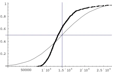
Unfortunately a special problem arises in application of this method when summing samples from the lognormal distribution, or any other distribution where g(x) is a power function like 10x. Such a distribution has an extremely long tail. In a Monte Carlo (or Latin Hypercube) sample the probability of sampling from this tail is extremely low. However, the large values in this tail are dominating the size of the (analytic) variance of the distributions: the variance in a sample from a lognormal distribution is much lower than the analytic variance. The result is that the value of N’ = ΣnNi may be too large when it is approximated by sampling from a

N(nµ,σ√n) distribution, derived by using the central limit theorem and equations (2.17) through (2.20). As illustrated below, it implies that we cannot use this approximation when n is (relatively) small. In that case, simulation is the only option.

For example, consider n broccoli trunks. The distribution of the number of spores per trunk is known to be lognormal, characterised by a probability density function f(x) = N(2,1) and the transformation function g(u) = 10u . This implies that the median number of spores is 102, and by calculating equations (2.19) and (2.20) it can be derived that µ =102 + ln(10)/2 _{≈ 1417 and σ}

= √ (104 + 2 ln(10)_-104+ln(10)_{) ≈ 20022. We are now interested in the probability distributions of}

the number of spores in batches of both n=100 and n=1000 broccoli trunks.

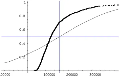
In figures 2-5 and 2-6 the result of 1000 Monte Carlo’s (MC’s) with n=100 and n= 1000 iterations is compared with the Normal N(nµ,σ√n) distribution that the central limit theorem (CLT) predicts. Each MC predicts a random batch. The results of the MC’s are sorted and

-100000 100000 200000 300000 0.2 0.4 0.6 0.8 1

Figure 2-5 Comparison of Monte Carlo results and the prediction using the central limit theorem with n=100. The cumulative distribution is shown with the sum of spores on the x-axis and the probability on the y-x-axis. For the MC the mean is 13.9×104_{, the median is}

10.3×104 _{and the standard deviation is 12.9×10}4_{. For the CLT method the mean and median}

500000 1´106 1.5´106 2´106 2.5´106 0.2 0.4 0.6 0.8 1

Figure 2-6 Comparison of Monte Carlo results and the prediction using the central limit theorem with n=1000. The cumulative distribution is shown with the sum of spores on the x-axis and the probability on the y-x-axis. For the MC the mean is 14.1×105_{, the median is}

13.1×105 _{and the standard deviation is 47.3 .10}4_{. For the CLT method the mean and median}

are 14.2×105_{, and the standard deviation is 63.3×10}5_.

plotted on a scale from 0 to 1, so that, when the two methods match, the MC should largely overlap the normal distribution predicted by the CLT. The figures illustrate that this is not the case. The median and the standard deviation of the MC-distribution is lower than predicted by applying the CLT. This effect is largest when n is relatively small.

The problem outlined above, that the sum of a (large) number of samples from a lognormal or similar long tailed distribution can not be predicted by a known distribution, may be solved by selecting the Gamma distribution as the initial distribution (for e.g. the number of cfu on the broccoli trunks). When n samples from a Gamma distribution Γ(α,β) are summed up, this sum is Γ(αn,β) distributed (Johnson and Kotz 1970), which is easy to implement in a spreadsheet. However, the choice for a Gamma distribution must be realistic: data or expert opinion must be in accordance with the shape of the Gamma distribution. In this context, an important feature of the Gamma distribution is that, if the standard deviation is larger than the mean (as in the example discussed above), the mode of the distribution is at zero. This means that if the initial distribution has a long tail (so the standard deviation is large) and a most likely value larger than zero, the gamma distribution cannot be applied.

2.3.2.5 Removal

Removal is a process where some units (or parts of units) are selected and removed from the production process. Examples are the rejection of carcasses by veterinary inspectors in the slaughter house or the discarding of ‘ugly’ vegetables. If the removal would be a random process, it would have no effect on the risk assessment. However, the process is usually

performed because there is a presumed relation with microbial contamination: (heavily) contaminated units are discarded more often than lightly or non contaminated units.

A graphical representation is given in Fig 2-7

c

c

c

c

Figure 2-7 In the basic process ‘removal’ a fraction of the units is removed from the food pathway. Contaminated units (marked ‘c’) are removed with a higher probability than units that are not contaminated (not marked.) Typically, removal is a selection procedure based on e.g. visible effects of contamination.

Removal is often a subjective process in which the relation between rejection and level of contamination is obscure. Therefore useful mechanistic modelling of the removal process is complex. The simple model presented below is sufficient so far and may be improved in the future.

If it is assumed that heavily contaminated units are not discarded with a higher probability than lightly contaminated units, removal only affects prevalence, and not the variability distribution of the number of cells over the units. In that case removal can be represented by a factor f, such that the prevalence P` after removal is equal to

P`=P.f / (1-P+Pf) with 0≤ f ≤1 (2.21)

The rationale behind this equation is shown when (2.21) is rewritten as P`/P = f (1-P`)/(1-P), or by expressing f as f = (1-pc)/(1-pnot c), with pc the probability of removal of a contaminated unit and pnot c the probability of removal of a not contaminated unit. If f=0 all contaminated heads are removed, if f=1 none of them are removed.

This f may be variable and uncertain, derived from experimental results or expert opinion.

2.3.2.6 Cross contamination

Cross contamination is an important process in food safety, but not well-defined. Several types of cross contamination can be considered. Cross contamination can be the direct transmission of cells from one unit to another, e.g. by the (short and incidental) physical contact between two animals, carcasses, vegetables etc. It can also be indirect transmission, for example via the hands or equipment of a food processor. A third type of contamination is the transmission from outside the food production process, the introduction of cells from vermin, dirty towels etc. Strictly speaking, this is not ‘cross’ contamination. It may be an important process if it refers to the introduction of (substantial quantities of) the hazard

considered into the food chain. If it is believed to be relevant, it should be incorporated in the exposure assessment separately.

Ignoring this last type of cross contamination, these cross contamination processes have in common that the prevalence is increased and that the number of cells remains about equal, and is only somewhat redistributed between the units.

For the prevalence we can then apply the same equation (2.21) as for removal, but now f>1 (Cassin et al. 1998a, Fazil, A. and Lammerding, A., unpublished):

P`=P.f/(1-P+Pf) with f>1 (2.22)

The larger f, the larger the impact of cross contamination. Like in the case of the removal process, this f may be variable and uncertain, derived from experimental results or expert opinion. Whether the effect of cross contamination on N is important, and how it is to be modelled, depends on the specific situation analysed.

2.3.2.7 Black Box

As stated above, some processes are to be regarded as ‘black boxes’. A process like defeathering in a poultry slaughterhouse, for example, holds elements of removal, cross contamination and possibly involves growth or inactivation. If there is no proposal for an alternative scenario including this processing step, and the knowledge about its potential effects on the microbial hazard considered is limited, this might be regarded as ‘one processing step’. The transmission is most easily modelled by linear models, that is by assuming that the number of cells changes by an uncertain and possibly variable factor: N’ =

N.x, so

log (N’) = log (N) + x , (2.23)

with x a real number), and that the prevalence may change with a factor as modelled in the removal and cross contamination basic processes

P`=P.f/(1-P+Pf) with f>0. (2.24)

The values of these factors will have to be estimated by data from the process considered or expert opinion. In both cases variability and uncertainty will have to be incorporated explicitly in the model. If there are a series of input-output data available, these may show that the input output relation is not linear. In that case another relation will have to be modelled, if possible with a mechanistic model, including relevant parameters.