BioScore 2.0, a species-by-species model to assess anthropogenic impacts on terrestrial biodiversity in Europe

(1)

BIOSCORE 2.0

A species-by-species model to assess anthropogenic

impacts on terrestrial biodiversity in Europe

Marjon Hendriks, Arjen van Hinsberg, Peter Janssen and Bart de Knegt (Eds.) December 2016

(2)

BioScore 2.0: A species-by-species model to assess anthropogenic impacts on terrestrial biodiversity in Europe

The Hague, 2016

PBL publication number: 2501

Corresponding author

Marjon.Hendriks@pbl.nl

Authors

Marjon Hendriks1_{(eds), Jan Clement}2_{, Moreno Di Marco}3_{, Stephan Hennekens}2_{, Arjen van}

Hinsberg1_{(eds), Mark Huijbregts}1_{, Peter Janssen}1_{(eds), Christian Kampichler}4_{, Bart de}

Knegt2_{(eds), Onno Knol}1_{, Sido Mylius}1_{, Wim Ozinga}2_{, Rogier Pouwels}2_{, Carlo Rondinini}3_{, Luca}

Santini3_{, Joop Schaminée}2_{, Aafke Schipper}1_{, Henk Sierdsema}4_{, Chris van Swaay}5_{, Sandy van}

Tol1_{, Hans Visser}1_{, Jaap Wiertz}1

1_{PBL Netherlands Environmental Assessment Agency} 2_{Wageningen University & Research}

3_{Sapienza University (Global Mammal Assessment)} 4_{European Bird Census Council (Sovon, NL)}

5_{Butterfly Conservation Europe (Vlinderstichting, NL)} Acknowledgements

We thank all colleagues from PBL Netherlands Environmental Assesesment Agency,

Wageningen University & Research, Sapienza University, European Bird Census Council and Butterfly Conservation Europe for their contribution and comments.

Graphics

PBL Beeldredactie

Production coordination

PBL Publishers

Parts of this publication may be reproduced, providing the source is stated, in the form: Hendriks M. et al. (2016), BioScore 2.0: A species-by-species model to assess anthropogenic impacts on terrestrial biodiversity in Europe, PBL Netherlands Environmental Assessment Agency, The Hague.

PBL Netherlands Environmental Assessment Agency is the national institute for strategic policy analysis in the fields of the environment, nature and spatial planning. We contribute to improving the quality of political and administrative decision-making by conducting outlook studies, analyses and evaluations in which an integrated approach is considered paramount. Policy relevance is the prime concern in all of our studies. We conduct solicited and

(3)

Preface

The BioScore model (Biodiversity impact assessment using species sensitivity Scores) has been developed in order to provide a tool able to assess the impacts of policy measures on biodiversity in Europe. BioScore projects the spatial distribution of individual species (plants, invertebrates and vertebrates) in relation to a set of environmental factors related to

climate, soil, land use and various human-induced pressures, including acidification, eutrophication and habitat fragmentation. The first version of the model was released in 2009, resulting from a research project funded by EC DG Research and Technological Development FP6 (www.bioscore.eu). The project was coordinated by the European Centre for Nature Conservation (ECNC) / Ben Delbaere and executed by a consortium of nine partners. PBL Netherlands Environmental Assessment Agency and Alterra Wageningen UR were in charge of the development of the BioScore database and web tool (Delbaere et al., 2009).

BioScore version 1.0 has been used for a number of Europe-wide scenario studies. PBL has been developing an improved version of the model (BioScore 2.0), based on the experiences with BioScore 1.0 and a list of proposed model improvements as identified in Delbaere et al. (2009). Compared to the previous version, BioScore 2.0 is based on improved species monitoring data and improved response relationships to describe species’ probability of occurrence in relation to the environmental factors of concern. The following partners have been highly involved in the development of BioScore 2.0:

• European Bird Census Council / Henk Sierdsema, Sovon (NL);

• Butterfly Conservation Europe / Chris van Swaay, Vlinderstichting, (NL);

• European Vegetation Survey / Stephan Hennekens and Joop Schaminée, Alterra, (NL);

• Global Mammal Assessment / Luca Santini and Carlo Rondinini, Sapienza University, (IT).

An important application of BioScore 2.0 has been in PBL’s Nature Outlook 2016. The Nature Outlook studies are produced every four years. They provide perspectives on nature and policy options for the next 30 to 40 years. Until now, these assessments have been limited to the Netherlands. However, as national nature policy is increasingly decided upon at EU level, the Dutch Government has requested PBL to expand the study area to cover the whole of the EU-28.

This report describes the model concept and methodology underlying BioScore 2.0, and illustrates the type of results that can be obtained with the model. Furthermore, it discusses both the methodology and the results.

(5)

Summary

BioScore 2.0 is a model which supports the analysis of potential impacts of future changes in human-induced pressures on European terrestrial biodiversity (e.g. mammals, vascular plants, breeding birds and butterflies). The model is based on large databases on species occurrences in Europe. The relationship between species observations and pressures is calculated through statistical analysis. By using output of models on future changes in pressures, BioScore 2.0 can be used for calculating changes in species occurences. In this way, BioScore 2.0 can be used for assessing policy plans or scenarios on the achievement of European biodiversity goals and on impacts of climate change. It models changes in both species abundance and habitat quality. This is of interest to policymakers and scientists. BioScore 1.0, released in 2009, resulted from a research project funded by EC DG Research and Technological Development, FP6 (www.bioscore.eu). The project was coordinated by the European Centre for Nature Conservation (ECNC) and executed by a consortium of nine partners. PBL has been developing an improved version of the model (BioScore 2.0), together with European Bird Census Council (Sovon), Butterfly Conservation Europe (De Vlinderstichting), European Vegetation Survey and Sapienza University.

The driving variables included are climate change, land-use change, and local environmental pressures. The last include air pollution through nitrogen and sulphur deposition, agricultural intensification, water stress, habitat fragmentation, forest and nature management, and disturbance caused by roads and urbanisation. The model assesses the impacts on

probability of occurrence for 1400 policy-relevant species, for each 5 x 5 km grid cell. Model calculations are executed in five consecutive steps. In the first step, climate, elevation and soil maps are used to project the distribution range of each species. The second step uses land-cover information to determine suitable habitats, per species, within their distribution range. In the third step, the relationships between local pressures (e.g. water stress and habitat fragmentation) and species occurrences are derived. In the fourth step, the relationships between local pressures and species occurrence are combined with species distribution ranges and species habitat suitability, in order to produce probability maps of species occurrence. In the final step, these maps are aggregated into species and ecosystem indicators.

This report provides detailed descriptions of the calculation procedures in the five steps and the data used in each step. It discusses the quality and applicability of BioScore 2.0.

(6)

1 Introduction

Global biodiversity is currently declining at an unusually high rate (Butchart et al., 2010; Barnosky et al., 2011; Pereira et al., 2012; Tittensor et al., 2014). This brings about a clear demand for quantitative models able to project future biodiversity in response to

anthropogenic pressures as well as policy measures designed to counteract the decline (Pereira et al., 2010; Harfoot et al., 2014a). Common biodiversity modelling approaches range from descriptive correlative statistical models, such as species distribution models (SDMs) or species–area relationships (SARs), to more mechanistic, process-based models that simulate population or community dynamics (Boyce, 1992; Drakare et al., 2006; Elith and Leathwick, 2009; Harfoot et al., 2014b). As process-based models tend to be more data and computationally intensive, large-scale biodiversity assessments are commonly based on correlative models.

In general, there are two main approaches to correlative biodiversity modelling. In the first approach, biotic survey data are aggregated to location-specific estimates of assemblage-level biodiversity indicators, such as species richness or mean species abundance (MSA) (Thomas et al., 2004; Alkemade et al., 2009). These indicators are then used to establish quantitative cause–effect relationships by relating them to measurements or estimates of co-occurring environmental factors (‘assemble first, predict later’; (Ferrier and Guisan, 2006)). In the alternative approach, the environmental responses of the individual species are modelled first, by establishing so-called species distribution models (SDMs) or habitat suitability models (HSMs), i.e., quantitative relationships between the abundance or (potential) occurrence of a species on the one hand and a set of environmental factors on the other (Elith and Leathwick, 2009). The modelled species' or habitat distributions are then combined in order to derive multi-species biodiversity indicators (‘predict first, assemble later’ (Ferrier and Guisan, 2006)).

Modelling individual species is a very flexible approach to biodiversity modelling: once the distributions of the individual species are known, virtually any property of an assemblage and hence virtually any multi-species biodiversity indicator can be derived (Ferrier and Guisan, 2006). Moreover, species-specific models are expected to improve our understanding and predictive ability of ecological responses to global change, as they allow for evaluation of which species are at higher risk and why (Visconti et al., 2016b). So far, however, a species-by-species approach to biodiversity modelling has mostly been restricted to relatively few species, to particular taxonomic groups, or to relatively few environmental factors, mostly related to climate change and land use (Thuiller et al., 2005; Visconti et al., 2011; Feeley et al., 2012; Ficetola et al., 2015; Visconti et al., 2016b).

The BioScore model was developed with the aim to establish a large-scale species-specific biodiversity assessment model including species from multiple taxonomic groups and a set of environmental factors representative of a variety of anthropogenic pressures. The model was specifically designed to quantify the impacts of policy measures on biodiversity in Europe (Delbaere et al., 2009). A first version of the model was released in 2009. The present report describes version 2.0 of the BioScore model, which was developed based on the experiences with version 1.0 and a list of improvements proposed upon completion of version 1.0

(Delbaere et al., 2009). Compared to the previous version, BioScore 2.0 is based on improved species monitoring data and improved response relationships to describe species’ probability of occurrence in relation to the environmental factors of concern. BioScore 2.0 projects the spatial distribution of individual species belonging to four taxonomic groups

(7)

(vascular plants, butterflies, breeding birds and mammals) in relation to a set of environmental factors related to climate, soil, land use and various human-induced pressures, including acidification, eutrophication and habitat fragmentation. It includes a total of 1320 policy-relevant species, of which 863 vascular plants, 95 butterflies, 284 breeding birds and 78 mammals.

(8)

2 Methods

2.1 General approach

BioScore follows a hierarchical approach to species distribution modelling, assuming that the distribution of a species results from a set of nested environmental filters ranging from large-scale climatic and soil variables at the coarsest spatial resolution via land cover and land use to fine-grained habitat characteristics at the highest spatial resolution (Pearson and Dawson, 2003). First, the distribution range of each species is projected based on envelope models that estimate species’ probability of occurrence in relation to large-scale climate and soil characteristics (Figure 2.1). From the projected envelopes, the areas with potentially suitable habitat for each species are selected based on its affinity to specific land-cover, land-use and/or land-management types. Thirdly, the species’ probabilities of occurrence within the potentially suitable habitat are determined based on their responses to environmental factors indicative of various human pressures, including habitat fragmentation, eutrophication and acidification.

Model results are then aggregated by location and/or species, in order to obtain species and ecosystem indicators (Figure 2.1). Species indicators give an indication of the percentage of species changing, where change of a species is determined by the change in summed probability of occurrence over all grid cells. The ecosystem indicators give an indication of changes in ecosystem quality, where change of quality is determined by the sum of occurrence probability of all species per grid cell.

Figure 2.1: Conceptual scheme of the BioScore model, showing a hierarchical approach to biodiversity modelling where the occurrence probability of each species is a function of a set of nested environmental filters including large-scale climate and soil characteristics (step 1), land use (step 2) and fine-grained environmental characteristics influencing habitat quality (step 3).

(9)

2.2 Species

2.2.1 Species selection

Selection of taxonomic groups

BioScore 2.0 focuses on species relevant for European policies, i.e. species mentioned in the Birds and Habitats Directives (or underlying lists of the Bern Convention) and/or Red Lists, or species considered to be characteristic for the selected Annex I habitat types. The Birds Directive aims to protect all European wild birds throughout their natural range within the EU. It also identifies 193 species and subspecies of wild birds naturally occurring in Europe as being in need of special conservation measures. These species, listed in Annex I of the directive, are considered to have the following characteristics: to be in danger of extinction, to be vulnerable to specific changes in their habitat, to be rare, or to require specific

attention because of their habitats. The Habitats Directive aims at ensuring the conservation of a variety of rare, threatened, or endemic species, including more than 1250 species and subspecies and 237 habitat types. The quality of the habitat types are measured by so-called typical species. Full lists of typical species do not exist. However manuals are available to help Member States listing these species. Based on available information it is clear that most typical species are plant species, but also butterflies are often mentioned.

BioScore 2.0 focusses on terrestrial biodiversity and four groups which are of prime importance of the Birds and Habitats Directives, i.e. the vascular plants,

butterflies, mammals and breeding birds. This of course holds for the breeding birds protected in the Birds Directive. Plants have the longest list of protected species in the Habitats Directive and mammals and arthropods (including Butterflies) are the next groups in size.

Within these four taxonomic groups, the species were selected based on both policy relevance and availability of monitoring data. A list of criteria specific to each taxonomic group is provided below:

Vascular plants

First, 40 protected terrestrial habitat types were selected (Hennekens et al., 2015); • The habitat is terrestrial and listed in the Habitats Directive, and the habitat is not

confined to local sites but relevant across Europe and well characterised from a phytosociological point of view. (Some habitats for which the Netherlands has an

international responsibility, especially wetlands, dunes and heathland were also selected in order to enable Dutch assessments).

• The set of habitat types is selected to be representative of the variation in main habitat types across Europe (i.e., including coastal habitats, grasslands, fens and forests). • The set of habitat types includes High Nature Value (HNV) Farmland (Paracchini et al.,

2008).

Next, for each habitat type a set of typical species was selected, using the ‘Interpretation manual of European habitats’ as starting point (EC, 2013). If this did not provide sufficient and correct information on typical species, information was added from unpublished synoptic tables of alliances from the ‘EuroVegChecklist’ and other literature. More recently 5 extra habitat types were selected, with characteristic species, but these have not yet been included in the model. These habitat types are H1340 ‘Inland salt meadows’, H5110 ‘Stable

xerothermophilous formations with Buxus sempervirens on rock slopes (Berberidion p.p.)’, H7140 ‘Transition mires and quaking bogs’, H9110 ‘Luzulo-Fagetum beech forests’ and H91H0 ‘Pannonian woods with Quercus pubescens’.

(10)

Butterflies

Butterfly species were selected when fulfilling at least one of the following criteria (Van Swaay et al., 2014):

• The species is listed in the annexes II and IV of the Habitats Directive or the species is a ‘typical species’ for at least one of the habitats mentioned in Annex I of the Habitats Directive.

• The species occurs on the European Red List as Near Threatened (NT), Vulnerable (VU), Endangered (EN) or Critically Endangered (CR).

• The species is used for the identification of High Nature Value (HNV) Farmland (Paracchini et al., 2008).

• Monitoring data should be available from at least 50 transects (see Section 2.2.2). In addition;

• The species occurs in more than one biogeographic region throughout Europe. (Some species should be characteristic of one of the habitat types for which the Netherlands has an international responsibility, especially wetlands, dunes and heathland in order to enable Dutch assessments).

• The species has a high area under the ROC curve (AUC >0.75) in the climate models of Settele et al. (2008), and thus can be modelled using climate-change models.

• The species is assessed in BioScore 1 (see www.bioscore.eu).

Breeding birds

Breeding bird species were selected when fulfilling at least one of the following criteria (Sierdsema, 2014):

• The species is mentioned in the Birds Directive

• The species is a target species for the designation of Special Protection Areas (SPAs) according to the Birds Directive.

• The species is characteristic of High Nature Value Farmland Farmland (Paracchini et al., 2008).

In addition;

• The species is included in BioScore 1.0 (see www.bioscore.eu), except if it does not breed in the geographical range of interest (mainly species breeding in the Siberian arctic). • Some species associated with old growth forest.

• Species can be modelled with climate-change models and are expected to be

disproportionally impacted by climate change (mainly boreal, arctic and alpine species).

Mammals

Mammal species were selected when fulfilling at least one of the following criteria (Hennekens et al., 2015):

• The species is listed under the Habitats Directive. • The species is listed under the Bern Convention. • The species is listed under the Bonn Convention. • The species is listed under CITES.

• The species is considered threatened according to the IUCN Red List (categories Vulnerable (VU), Endangered (EN) and Critically Endangered (CR)).

And:

• species should be monitored in a sufficient number of high-quality presence points (see further Section 2.2.2).

Based on these criteria, a total of 1402 species were initially selected for inclusion in BioScore 2.0 (see Table 3.1).

(11)

2.2.2 Species monitoring data

Species observations were obtained from various sources, including point record databases, atlas data and range maps (Table 2.1). For butterflies and breeding birds, different data sources were used for the different modelling steps. For the first step, the distribution range modelling, atlas data with a 50 km resolution were used, covering the same time period as the data used for the climate-related predictor variables. For the second and third steps, which require species observations at higher resolution, point records were used. For vascular plants and mammals, point records were used for all three steps.

Point observations were retrieved/selected as follows:

• For plants species, observations in geo-referenced vegetation plots from the European Vegetation Archive (EVA) were used as a basis, supplemented with geo-referenced point observations from GBIF to complement data in regions where EVA has less data coverage (Hennekens et al., 2015).

• For butterflies, monitoring transect data were used from seven countries/regions engaging in Butterfly Monitoring Schemes: Finland, Germany, Netherlands, United Kingdom, France, Catalonia and Sweden. Data for in total 3000 transects were available for 2010–2012 (Van Swaay et al., 2014).

• For breeding birds, only point records were selected that were not further than 50 km from the species ranges as mapped by Birdlife International. To ensure that the

observations concerned only breeding birds, for migratory species only observations were selected from a species-specific window representing the breeding season (Sierdsema, 2014).

• For mammals, a selection was made for records obtained after 1990, with a spatial precision of <10 km and falling within the species' geographic range as available from IUCN (www.iucn.org). This resulted in a total of 81 species for the analyses, with a minimum of 29 presence points and a maximum of 9,899 points per species (Hennekens et al., 2015).

Table 2.1: Data sources, number of species observations present in the database and modelling steps in which the data are used. Step 1 refers to the models describing the species’ distribution range, step 2 refers to the selection of potential habitat, and step 3 refers to the calculation of the pressure–response curves (see also Figure 2.1).

Data source No. of observations Used in step

Vascular plants

European Vegetation Archive

(http://euroveg.org/eva-database)

20.5 million

1, 2, 3 Global Biodiversity Information Facility

(www.gbif.org) 22 million 1, 2, 3

Butterflies

LepiDiv database (UFZ, Leipzig-Halle) (Kudrna et

al., 2011) 137 to 2119 per species 1

IUCN range maps (www.iucn.org) Not applicable;

polygons 1

- database created within project LOLA (www.cesab.org)

- Svensk Dagfjärilsövervakning (www.dagfjarilar.lu.se/)

95,000 2, 3

Breeding birds

EBCC Breeding Bird Atlas 1980–1995

(www.ebcc.info) 1,351,000 1

eBird (www.ebird.org) 23,706,000 2, 3

Global Biodiversity Information Facility

(12)

Data source No. of observations Used in step

Observado and waarneming.nl

(www.observado.org) 23,706,000 2, 3

Distribution maps for EU N2000 reporting (Article

12 BirdsDirective) (www.eea.eu) 28,020,000 2, 3

Bulgarian bird counts

(pc.trektellen.nl) 202,000 2, 3

Mammals

Global Biodiversity Information Facility

(www.gbif.org) 179,000 1, 2, 3

Observado (www.observado.org) 14,000 1, 2, 3

Silene database 8,000 1, 2, 3

Sicily atlas 2,700 1, 2, 3

Repertorio Naturalistico Toscana (re.na.to) 1,300 1, 2, 3

French national bat atlas 41,000 1, 2, 3

Derived from research papers 1,500 1, 2, 3

Private GMA database 4,600 1, 2, 3

2.3 Environmental variables

The usefulness of an assessment tool such as BioScore will increase when policy makers are informed about the potential effects of decisions. With respect to stopping the loss of biodiversity or reaching the targets of the Birds and Habitats Directives, it is not only important to look at the ecologically important factors, but also to incorporate factors mentioned in policy. In BioScore 1.0, 26 legislative documents were screened for mention of any environmental variable or pressure on biodiversity (Delbaere et al., 2009). At the same time, ecologically relevant factors were listed for modelling species occurrences.

Variables for modelling the distribution range (step 1)

For the envelope models, climate variables were selected according to the following criteria, which all needed to be fulfilled (Hennekens et al., 2015):

• Ecologically relevant, and used in other climate studies, for at least one of the species groups (Bakkenes et al., 2002; Huntley et al., 2007; Settele et al., 2008).

• Available at high resolution for EU28 (preferably 1 x 1 km).

• Computable with models, in order to facilitate climate-change projections.

Climate variables were retrieved from the BioClim database (Hijmans et al., 2005). Based on the four criteria listed above, seven climate variables were selected from the 19 variables available in BioClim (Table 2.2). To the BioClim data, temperature sum in the growing season and the annual ratio of actual to potential evaporation were added from the IMAGE model (Bouwman et al., 2006).

Soil variables are included to model the distribution range. Selected variables were acidity, soil moisture content, organic carbon content in the top soil, clay content in the top soil, silt content in the top soil and availability of salt. These soil factors were expected to be most important for the distribution of plants and habitats and indirect for the animal species living in those habitats. In addition, elevation was added to this list.

Variables to model the extent of suitable habitat (step 2)

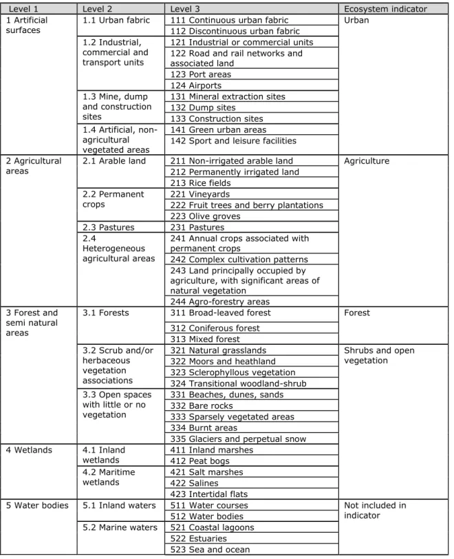
Land-cover data, needed for the habitat modelling in step 2, was retrieved from the CORINE land-cover (CLC) map of the European Environment Agency for the year 2000, combined with information from the Pan-European Land Cover database (PELCOM) of Alterra and the Global Land Cover 2000 (GLC2000) map produced by the Joint Research Centre (Table 2.2) (Hazeu et al., 2008). The thematic classification of the map corresponds with the CLC

classification (Appendix I). The map was aggregated from 100 metres to a resolution of 1 km by selecting the class which covered the majority within the 1km grid cell.

(13)

Variables to model the quality of the habitat: Pressure variables (step 3)

The selection of pressure variables (step 3) was based on the following criteria, which all needed to be fulfilled:

• The pressure is known to affect species’ occurrence or habitat quality and/or the pressure is considered relevant in European policies and goals (Delbaere et al., 2009).

• High-resolution data is available for the pressure of concern.

• The pressure can be modelled, in order to facilitate scenario projections.

In BioScore 1.0, 26 legislative documents were scanned in order to identify policy-relevant instruments and drivers. This exercise resulted in a list of over 200 terms, ranging from ‘abandonment of high-nature-value farmland’ (EC Biodiversity Communication, 2006) to ‘wind’ (EC Biodiversity Strategy, 1998). The list contained very specific activities with direct pressures related to them, such as ‘ammonia and nitrous oxide emissions to air’ (Thematic Strategy on Air Pollution 2005). It also contained broader terms such as ‘use of fossil fuels’ (Thematic Strategy on the Urban Environment 2005) or even very general terms such as ‘climate change’ (various instruments). These different drivers and pressures were divided into 11 groups of policy-relevant drivers/environmental pressures, i.e. climate change, land-use change, pollution, fragmentation, disturbance, direct pressures, species interaction, management, water , water-related changes and miscellaneous (Delbaere et al., 2009). Ecologically relevant factors, such as natural geological events and catastrophes, were excluded. Because of data availability species interactions (e.g. effects of invasive and introduced species) were also excluded. Eventually 8 pressure variables were selected (Table 2.2). Total deposition of oxidised sulphur and total deposition of nitrogen were selected to incorporate the most important effects of pollution (eutrophication and acidification) on natural ecosystems. Acidification and eutrophication due to atmospheric sulphur and nitrogen deposition threatened Europe’s natural areas and directly influences plant species occurrence (Galloway, 1984; Slootweg et al., 2014). These factors are also used for modelling effects in animals, as changes in vegetation may influence animal species occurrence. Nitrogen input was chosen as an indicator for agricultural intensification. Nitrogen input includes manure application (corrected for volatilisation losses), manure deposition by grazing animals and the application of mineral fertilizer. Desiccation was chosen as an indicator of influence of water use. Proximity of roads and urban land use was used as an indicator for various disturbances due to human activities which can’t be modelled in detail, such as noise, light and traffic.

To assess the impact of fragmentation the spatial cohesion of ecosystems was used. This spatial cohesion was determined by LARCH-SCAN (Appendix II) (Groot Bruinderink et al., 2003; IEEP and Alterra, 2010). For fragmentation, for each species of plants, birds and butterflies out of a set of 24 maps one map was selected as a measure for the spatial cohesion of its habitat (see Section 2.4.3). The set of 24 maps covers six ecosystem types/land-cover classes and four possible dispersal distances (10, 20, 50 and 100 km). Land-cover classes include forests (class 3.1), shrub and/or herbaceous vegetation (class 3.2), open spaces with little vegetation (class 3.3), inland wetlands (class 4.1), coastal wetlands (class 4.2) and open water (class 5.1). To create the fragmentation maps, the land-cover map was aggregated to a resolution of 1 x 1 km to express the amount of each of the six ecosystem types per grid cell. Then, the degree of fragmentation of each ecosystem type in each grid cell was calculated based on the amount of the same ecosystem type within approximately twice the dispersal distance. For each mammal species, a unique

fragmentation map was composed using LARCH-SCAN, land cover was synthesised of a set of the six ecosystem types/land-cover classes, depending on the habitat preferences of the species. The dispersal distance was selected based on the median dispersal distance as calculated in Santini et al.(2013). Little information was available on dispersal distance for most bat species, but as they are known to have good dispersal abilities, it was assumed that all bats are associated to max-grain fragmentation (100 km).

(14)

To quantify road impact, a selection was made of the primary, secondary and tertiary roads as included in the GRIP database (Meijer, 2009). A buffer zone of 500 meters was created around the roads and the total area of the buffer zone per 5 x 5 km grid cell was used as road impact indicator. To quantify urbanisation a similar approach was followed. From the land-cover map, all grid cells classified as urban were selected, a 500 m buffer was made around these areas and the total area of the buffer per 5 x 5 km grid cell was used as indicator of urbanisation.

Information on forest management was available as a 1 x 1 km map showing per cell one of the five potential forest management categories (close to nature; combined objective forestry; even-aged forestry; nature reserve; short rotation forestry). As the original map shows potential management types, locations without forest are also given a value. To cover actual forest only, all grid cells from the CORINE land-cover map not classified as forest were removed. Next, for each forest management category a map on a resolution of 5 x 5 km was constructed by aggregation from the underlying scales, rendering information on the area covered (within the 5 x 5 km grid cell) by this forest management category.

Table 2.2: Overview of the data used to quantify the environmental variables used in BioScore 2.0. For each variable the unit of the values in the map, the resolution of the map, the year the data is representative for and the source of the data are mentioned. More information on these variables can be found in Hennekens et al. (2015).

Variable Unit Resolution Year Source

Climate variables

Precipitation seasonality Mm 30 arc seconds ~1950–2000 BioClim1

Precipitation of driest month Mm 30 arc seconds ~1950–2000 BioClim1

Precipitation of warmest quarter

Mm 30 arc seconds ~1950–2000 BioClim1

Temperature seasonality °C * 10 30 arc seconds ~1950–2000 BioClim1

Isothermality °C * 10 30 arc seconds ~1950–2000 BioClim1

Min temperature of coldest month

°C * 10 30 arc seconds ~1950–2000 BioClim1

Mean temperature of driest quarter

°C * 10 30 arc seconds ~1950–2000 BioClim1

Temperature sum in growing season

°C 0.5 arc degrees 2010 IMAGE model

(version 2.4)2

Annual ratio of actual to potential evapotranspiration

fraction 0.5 arc degrees 2010 IMAGE model (version 2.4)2

Soil variables

pH-H2O in top soil - 5 x 5 km 15 HWSD3

Availability of salt - 1 x 1 km 15 _{Sworld-soil map}4

Organic carbon content in top soil

% 1 x 1 km 15 _ESDB5

Clay content in top soil % 1 x 1 km 15 _ESDB5

Silt content in top soil % 1 x 1 km 15 _ESDB5

Elevation (elevation above sea level)

M 30 arc seconds 15 _SRTM6

Annual mean moisture index

fraction 10 arc minutes ~1950–2000 BioClim1

Land cover and management

Land cover - 100 m 2000 PLCM20007

Nature management of open vegetation

- No resolution Expert

(15)

Variable Unit Resolution Year Source

Pressure variables

Total deposition of oxidised sulphur

mg S/m2

1/16 degree 2009 LOTUS-EUROS9

model Total deposition of nitrogen mg

N/m2 1/16 degree 2009 LOTUS-EUROS model9 Nitrogen input in agricultural area kg N/ ha 1 x 1 km 2002 DNDC-CAPRI metamodel10 Desiccation (Water exploitation index per sub-basins of rivers)

fraction sub-basins of rivers 2006 LISFLOOD12

Fragmentation fraction 1 x 1 km 2000 LARCH-SCAN

model8 Forest management approach fraction 5 x 5 km ~2000– 200814 Derived from EFMM11

Impact of roads ha 5 x 5 km ~2005 Derived from

GRIP (version 1)13

Urbanisation ha 5 x 5 km 2000 Derived from

land-cover map

1_{(Hijmans et al., 2005);}2_{(Bouwman et al., 2006);}3_{Harmonized Soils World database}

(FAO/IIASA/ISRIC/ISSCAS/JRC, 2012); 4Not yet published; 5European Soil Database (Hiederer, 2013); 6_{Shuttle Radar Topography Mission data (Farr et al., 2007);}7_{Pan-European Land Cover Map (Hazeu et}

al., 2008); 8_{Management of open vegetation, such as natural grasslands and shrubs, excluding}

agriculture (Hennekens et al., 2015); 9 _{(Cuvelier, 2013), supplemented with (Benedictow, 2010);}10

(Leip, 2011) 11_{European Forest Management Map}_{(Hengeveld et al., 2012);}12_{(De Roo et al., 2012);}13

(Meijer, 2009) 14_{The forest management approach map is a map of potential forest management and is}

therefore not strictly representative for the forest management of this period. The input data on which the forest management approach map is based are mainly representative of the period 2000 to 2008. 15

Soil texture is assumed to not change within the time scale considered, between 2000 and 2050.

2.4 Species distribution modelling

2.4.1 Step 1: Species distribution range

In the first modelling step, the distribution range of each species within the study area is delineated based on envelope models that estimate species’ probability of occurrence (PoO) in relation to large-scale climate and soil characteristics. The models relating species occurrence probability to climate and soil variables were obtained with the boosted

regression trees technique (BRT) in the R environment (R Core Team, 2014). BRT constitutes a machine-learning non-parametric algorithm specifically suited to model nonlinear

relationships and interactions between predictors (Elith et al., 2008). BRT output includes information on the relative importance of each predictor as well as its marginal effect on the response, expressed by so-called partial dependence plots. For each species a BRT model was built with TRIM-Maps (Hallmann et al., 2015), a suite of R-scripts for creating

distribution maps from monitoring data and casual observations which employs functionality from related R-packages such as ‘dismo’ and ‘gbm’. Climate and soil variable data layers were resampled to a resolution of 5 x 5 km for plants, 50 x 50 km for butterflies and birds, and 10 x 10 km for mammals (Sierdsema, 2014; Van Swaay et al., 2014; Hennekens et al., 2015), reflecting differences in the resolution and accuracy of the species records. For the plants, butterflies and birds, absence data were available (i.e., vegetation plots or atlas blocks with absence values). For the mammals, 10,000 pseudo-absences were generated

(16)

across the study area (Barbet-Massin, 2012). Two sets of BRT models were established: one based on 10,000 randomly chosen absences and one based on 10,000 pseudo-absences selected using a sampling bias grid representing locations where a given species was not observed despite other similar species were present (Ranc et al., 2016). Per species, the best performing model of the two was retained, based on visual inspection of the

modelled distribution in comparison with the species’ range as delineated by IUCN (www.iucn.org).

Because of the large number of species involved, a uniform set of default BRT parameters was employed, consisting of a learning rate of 0.01 (which is used to shrink the contribution of each tree when added to the model, according to the idea that it is better to improve a model by taking many small steps than by taking fewer large steps), tree complexity of 2 (to allow for second order interaction terms), bag fraction of 0.75 (i.e. the fraction of the original data set which is randomly drawn for training additive tree models in each iteration of the stage-wise gradient step search), and the Bernoulli distribution family (because of the binary response data). BRT models were tenfold cross-validated for birds and fivefold for plants, butterflies and mammals. The predictive performance of the BRT models was assessed based on estimates of the area under the ROC curve (AUC) and the explained deviance of the cross-validated models.

For all species the probabilities of occurrence as predicted by the BRT models were translated such that probabilities below a species-specific threshold were set to 0 and probabilities above this threshold were retained for use in further modelling steps (see Section 2.4.4). For each species a probability threshold was determined that maximised the true skill statistic (TSS), as TSS has been shown to be one of the best measures for determining the threshold value for SDMs (Allouche et al., 2006). A weighted version of the TSS was used, according to:

TSSλ = λ·Sensitivity + Specificity – 1 (Eq. 1)

whereby a weighting factor λ higher than 1 puts more emphasis on correctly predicting presences, while a λ smaller than 1 puts more emphasis on correctly predicting absences. The value of λ was determined per taxonomic group, based on visual similarity with the known distribution of the species. A weighting factor λ = 1.1 for birds and λ = 1.2 for butterflies was deemed suitable for an appropriate discrimination between presences and absences by the species experts, while for mammals and plants sensitivity and specificity were weighted equally (λ = 1).

2.4.2 Step 2: Species suitability habitat

Filtering based on land cover

In the second step in the modelling approach of BioScore 2.0, the envelopes modelled in step 1 (consisting of the grid cells with PoO larger than the threshold) are refined by

selecting suitable habitats based on land cover. Species’ habitat preferences in terms of land cover were identified as follows:

• For plant species, habitat preferences were derived from the frequency of occurrence of each of the 40 selected Annex I habitat types in relation to each land-cover type (based on level 3 of the CORINE land-cover classification). A threshold of 5% was applied to determine which land-cover types were suitable for each habitat type. The match between habitat type and land cover obtained in this manner was checked by an expert and

further refined to exclude or include certain cover types per habitat type. The land-cover types suitable for each habitat types were then assumed to represent suitable habitat to all typical (i.e. habitat-related) species.

(17)

• For butterflies habitat preferences were determined by relating the species’ point observations to the land-cover map and selecting as suitable habitat for a species those land-cover classes (CLC level 3 containing at least 3% of the observations). The habitat suitability classification thus obtained was then checked by an expert to 1) exclude land-cover types erroneously assigned as suitable due to geo-referencing errors in the observations and 2) add land-cover types containing less than 3% of the records but known to be suitable to the species.

• For birds, information on habitat suitability was derived from Van Kleunen (2003), who defined the habitat use of all European breeding birds, in terms of EUNIS codes from regional and European atlases and literature. For implementation in BioScore, the EUNIS codes were translated to the classes of the CORINE land-cover map (see Appendix III for the conversion).

• For mammals, habitat suitability information was derived from Rondinini et al. (2011), who assessed the suitability of land-cover types as represented in ESA’s Global Land Cover map (Globcover) (version 2.1) for 5027 out of 5330 known terrestrial mammal species. For implementation in BioScore, the Globcover classes were translated to the classes of the CORINE cover map (see Appendix IV for the conversion). The land-cover classes that were classified as highly and medium preferred habitat by Rondinini et al. (2011) were considered suitable.

Influence of nature management of open vegetation

Because the suitability of any land-cover type for a particular species may depend on specific management measures (for example, some grassland species may occur only on grassland that is regularly mown), the extent of suitable habitat is further refined based on

management. This only applies to management of natural open vegetation, as agricultural intensification is already included in nitrogen input and forest management. Nature management applies to future situations (scenarios) only, i.e., it is not included when predicting the present-day or reference distribution of species. If a given scenario assumes that management is stopped (for example, cessation of mowing in abandoned grassland), the corresponding grid cells are removed from the habitat area of species dependent on management. The dependency of species on management is expressed as so-called

hemeroby level, which is an integer score ranging from 1 to 9 where 1 represents hemorobic (not dependent on human management) and 9 represents polyhemerobic (strongly

dependent on human activity). The assignment of hemeroby levels to habitat types is based on expert judgement. For the quantification of hemeroby levels on species level, the same selection of plots was used as for the other pressures. Each plant species was assigned a hemeroby level based on the habitat type of the plots in which the species occurs (mean value, see Annex 5 in (Hennekens et al., 2015)). Species with a hemeroby level above 5 were then classified as being dependent on management. For butterflies and birds the hemeroby classification was based on expert judgement. Mammal species are considered as not being dependent on management, hence the hemeroby filter is not applied. See

Appendix V for all species classified as dependent on management.

2.4.3 Step 3: Species response to pressures

Deriving pressure–response relationships

Pressure–response relationships were derived for each of the local-scale pressure variables nitrogen deposition, sulphur deposition, desiccation, nitrogen input, forest management, urbanisation, impact of roads, and fragmentation (Table 2.2). Variable maps were resampled to 5 x 5 km for plants, birds and butterflies and to 10 x 10 km for mammals taking the average value within a grid cell. Response relationships were obtained with logistic regression (logit link and binomial error distribution) in the R environment (R Core Team,

(18)

2014). Models with only a linear term as well as those with linear and quadratic terms were both considered, and the most parsimonious model per species and pressure was selected based on the Akaike information Criterion (AIC). Model performance was assessed by calculating AUC values based on a tenfold cross-validation.

Presence-absence data for this modelling step were retrieved as follows:

• For plant species, point records were selected located within the suitable habitat (determined in step 2) and within the limits of the binary map of the habitat type the species is characteristic for (determined in step 1). These occurrences were supplemented with a more or less equal number of randomly selected absences from the pool of

vegetation plots located within the same mask (Hennekens et al., 2015). (i.e., no pseudo-absences were generated)

• For the birds and butterflies, presence-absence data were retrieved from point record data sources within the species distribution range that contained true absences (Sierdsema, 2014; Van Swaay et al., 2014)

• For mammals, presences and absences were selected from the grid cells representing suitable habitat within the envelopes, using the distribution maps resulting from steps 1 and 2.

The response functions on average were computed on 9547, 405, 5898 and 3710 presence values and 12130, 551, 5898 and 3722 absence values for respectively birds, butterflies, mammals and plants. The exact number varies among species and pressures.

To select the appropriate layer with fragmentation for breeding birds, butterflies and plants (see Section 2.3), first all established relationships for fragmentation were discarded if both the linear and the quadratic term were not significant (p > 0.05). Secondly, the ecosystem type/land-cover class was chosen with the largest number of observations, as a proxy for the most important habitat of a species. A corresponding dispersal distance was then selected based on the goodness-of-fit of the regression model, selecting for each species the

fragmentation layer with the dispersal distance resulting in the model with the highest AUC.

Post-processing

Response relationships obtained for each species and pressure variable (excluding fragmentation, see above) were screened and selected/adjusted as follows:

• Relationships were only discarded if both the linear and the quadratic term were not significant (p > 0.05), indicating no significant response of the species to the variable of concern. Models with only a linear term relationships were discarded when the linear term was not significant (p > 0.05).

• Relationships including both a linear and quadratic term whereby the linear term was significant (p < 0.05) and the quadratic term resulted in a negative unimodal (U-shaped) response, were modified to include only the linear term (i.e., the coefficient for the squared term was set to zero). This was done for sulphur deposition, nitrogen deposition, nitrogen input, desiccation, impact of roads and urbanisation as these U-shaped types of responses are ecologically not expected for these pressures.

Based on the selected response relationships a probability of occurrence map per species per pressure was calculated.

Both the forest fragmentation maps and the maps of area covered per forest management approach are strongly correlated with the area of forest. To avoid that the effect of forest area shows up in two pressure–response relationships, thus acting as a clear confounder, the forest management maps have been aggregated to one forest management approach per 5 x 5 km grid. This correspond to the PoO with a 100% coverage of that management type from the pressure response curve. The forest management approach ‘combined objective forestry’ was much more abundant in the forest management map than the other approaches. To

(19)

avoid that this category becomes even more abundant, out of the other four approaches the dominant one is selected. All other grid cells are appointed to ‘combined objective forestry’.

2.4.4 Step 4: Probability of occurrence of species

The final step consists of combining the results obtained from steps 1–3. First, the results of steps 1, 2 and 3 are aggregated per species. For each species this results in a probability of occurrence per grid cell as a function of all the included environmental variables.

In order to aggregate over the environmental variables, for each species the model results from step 1 are combined with those resulting from step 3 in grid cells with land cover that is representing suitable habitat (delineated in step 2), as follows:

(Eq. 2)

where Odds represents the ratio p/(1-p) as calculated by the BRT (step 1) and logistic regression models (step 3). The use of odds enables to distinguish between the situation where a pressure decreases and where it increases the probability of occurrence. SF is a scaling factor calculated as the ratio N1/N0 of the number of presences and absences in the

species distribution data used in the corresponding modelling step. It reflects the simple null model (constant) and is used as a reference point to express how the Odds change relative to its average value (null-model reference point) due to the individual influences of the pressures.

A similar strategy is used to determine the Odds (p/(1-p)) which results from the combined influence of the environmental pressures modelled in step 3:

where Oddsk represents the ratio p/(1-p) for a given pressure k, according to the logistic

model which is established in step 3 for this single pressure–response relationship. The overall scaling SF1&3 is determined as the geometric mean of the separate scaling

factors:

A more extensive explanation of the derivation of Equations 2 and 3 is provided in Appendix VI.

The overall Odds from combining Equations 2 to 4 is then translated into an overall probability of occurrence, as follows:

Thus, the PoO represents the (conditionalised) probability of occurrence of a species in a specific land-cover type (step 2), under the prevailing conditions regarding climate and soil (step 1) and environmental pressures (step 3).

(20)

In the above integration, pressures are taken into account only in grid cells with land-cover types where the pressures are relevant. For example, forest management intensity is not relevant in agricultural areas. Table 2.3 shows the pressures included per land-cover type. Ecologically relevant pressures are included per land-cover type. For example forest

management is only included in forests. Nitrogen, sulphur deposition and fragmentation are not included in agriculture because these effects are expected to be negligible compared to the effect of agricultural intensity (mapped as nitrogen input).

As a final step in this integration to calculate the species PoO for a specific grid cell, one first determines what fraction of the grid cell is covered by the various land-cover types and then one calculates a weighted average of the species PoOs for the land-cover types of interest, using the fractions as weight factors in this averaging.

Table 2.3: pressures taken into account per land-cover type

Variable Urban area

(CLC class 1.X) Agriculture (CLC class 2.X) Forests (CLC class 3.1)

Shrubs and open vegetation (CLC class 3.2–5.1)

Climate and soil X X X X

Sulphur deposition X X X Nitrogen deposition X X X Nitrogen input X Forest management X Desiccation X X X Fragmentation X X Impact of roads X X X X Urbanisation X X X X Nature management X X

2.4.5 Step 5: Indicators on species and ecosystems changes

Biodiversity encompasses the overall biological variety found in the living world and includes the variation in genes, species and ecosystems. For this reason it is not possible to express biodiversity in one indicator only. Therefore a small number of complementary headline indicators were developed. The indicator at species level expresses the change in occurrence of species. The indicator at ecosystem level expresses the change in extent and quality of ecosystems, considering the change in probability of occurrence of all species occurring in that ecosystem. Four types of ecosystems were distinguished: shrubs and open vegetation (e.g. grassland), forests, urban areas and agricultural areas. Indicators can be presented as graphs or maps.

Maps with modelled probabilities of occurrence of each species for the reference year 2005 and a future scenario were then used to calculate indicators of biodiversity change on the level of species and ecosystems. In presenting the results the focus is on the relative change (change in the summed probability of occurrence between two scenarios).

Indicators can be calculated for specific selections of species (e.g. taxonomic groups, red list species) or a specific set of grid cells (e.g. Natura 2000 areas, countries, biogeographical regions) to increase policy relevance.

(21)

Species Indicator

Changes from the current situation to a future scenario in the summed probability of occurrence for each species was calculated. The proportion of species increasing or decreasing was expressed for the EU-28 plus Switzerland. The change in probability of occurrence per species was calculated as:

where Cs is the relative change in probability of occurrence of species S, PoOS,y and PoOS,0

are the probabilities of occurrence of species S in scenario year y and the reference year, respectively, and G refers to the number of grid cells in the study area. This is expressed in terms of percentage points.

Ecosystem indicator

In order to obtain an indicator on changes in the quality and extent of ecosystems, per grid cell, the relative change in summed probabilities of occurrence given the set of species considered was calculated between the current situation and a future scenario as follows:

where CG is the change in the sum of probability of occurrence in a grid cell G. All probability

of occurrences of all species are summed per grid cell. Changes are expressed as a product of the number of species and their change in probability of occurrence per 5 x 5 km grid cell. For expressing the change in quality and extent of the four distinguished ecosystems, the latter product is multiplied by the fraction covered by the specific ecosystem in the grid cell.

(22)

3 Model results

3.1 Species selection and relationships derived in steps 1,

2 and 3

Species selection

Models were retained for 1320 of the 1402 species that were initially selected (Table 3.1). All results presented consist of this selection of species. Species excluded were those for which no adequate climate/soil envelope could be established in step 1, based on visual inspection of the modelled distribution, or for which no model could be established due to lack of observations. Furthermore species were excluded when no pressure–response models were retained. The butterfly species Leptidea sinapis was discarded as recent research shows that this is a species complex consisting of at least three species (Dincǎ et al., 2011).

Table 3.1: Numbers of species initially selected for BioScore 2.0 and the numbers eventually included. A list of the species included is provided in Appendix V.

Species group Initial selection Final selection

Vascular plants 884 863

Butterflies 100 95

Breeding birds 299 284

Mammals 81 78

Total 1402 1320

Distribution models (step 1) and pressure–response relationships (step 3)

It is only partially possible to validate the model results obtained from applying BioScore 2.0, to the scenarios to assess the impact on species and ecosystems. Since no data on the future is available, one cannot test whether the BioScore 2.0 relationships between environmental conditions and species occurrence that are calibrated based on the species monitoring data will also hold under future conditions. Also there is limited possibility to compare BioScore modelling results by backcasting with information of the past, since historical data on species occurrences is scarce. Comparing the modelled output with that from other models provides information on model differences, but not on the quality of BioScore 2.0. What is left as a means of validation is cross-validation or with expert knowledge to assess its plausibility. Special points of attention is given to the relationships established in steps 1 and 3. The higher the plausibility and accuracy of these relationships, the more confident one could be in the predictive value of the model. Of course also due care should be taken when extrapolating the relationships for combinations of values of

explanatory variables outside the value range that has been used in estimating these relations.

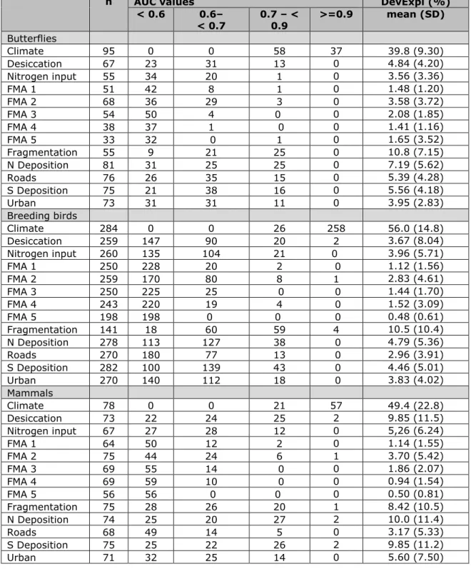
Cross-validation can be used as a first test to assess the predictive quality of the BioScore 2.0 model parts, albeit in conditions which reflect the present monitoring data. Table 3.2 shows the AUC and explained deviance of the models established in steps 1 and 3. For step 3 only the relationships are shown which are left after post-processing (see Section 2.4.3). An overview of the numbers of linear and quadratic pressure–response relationships obtained and the numbers resulting from the post-processing is provided in Appendix VII. As the

(23)

performance results in Table 3.2 show, the results of step 1 – where the influence of

climate–soil conditions on species occurrence is determined – show typically high (>=0.9) to moderate (0.7–0.9) AUC values, while the deviance explained is in the order of 40%

(butterflies) to 70 % (vascular plants), which indicates that a large part of the variation in the data on the scale under consideration can be explained already by the selected climate and soil variables. For the majority of the selected pressure–response relationships in step 3 the AUC values are lower than 0.7 and a mean explained deviance smaller than 10% (Table 3.2). These low explained deviance values are not surprising and are partly due to the fact that in each relationship only one variable was used, which describes generally less variation than a multitude of variables. Allowing for more complex model relations than the linear or quadratic forms which are used in the present single pressure logistic models could improve the statistical accuracy of these models.

When looking at the ecological plausibility of the pressure–response relationships of a few butterfly species the results are mixed (Swaay et al., 2016). Many relationships seem plausible, but there are also relations which seem unlikely. This means that a statistically inaccurate pressure–response relationship doesn’t always lead to an ecologically implausible relationship. However, more statistically accurate relationships will probably lead to more ecologically plausible relationships.

Habitat preference (step 2)

Most species can occur in forest and other terrestrial nature areas (CLC code 311–333). Fewer species had a habitat preference for agricultural area (CLC code 211–244) or wetlands and open waters (CLC code 411–523). There were no plant species with a habitat preference for urban areas (CLC code 111–142) and few bird, mammal and butterfly species with this preference (Table 3.3).

Table 3.2: Overview of performance for the models established for steps 1 and 3 for each of the four taxonomic groups. For step 3 only the selected pressure–response relations are shown (see ‘post-processing’ in Section 2.4.3) The number of models is shown as well as the distribution of AUC values validated models), the average explained deviance (cross-validated models) and the standard deviation of the explained deviances. FMA refers to forest management approach, with 1 = close to nature, 2 = combined objective forestry, 3 = even-aged forestry, 4 = nature reserve, 5 = short rotation forestry).

n AUC values DevExpl (%)

< 0.6 0.6– < 0.7 0.7 – < 0.9 >=0.9 mean (SD) Vascular plants Climate/soil 863 0 1 3 859 68.5 (13.8) Desiccation 719 420 196 98 5 5.48 (9.14) Nitrogen input 742 334 266 136 6 6.30 (8.82) FMA 1 652 545 98 9 0 1.82 (3.12) FMA 2 714 460 193 61 0 3,65 (5.29) FMA 3 604 506 86 12 0 1.80 (3.46) FMA 4 641 535 88 18 0 2.13 (4.62) FMA 5 501 499 1 1 0 0,69 (1,19) Fragmentation 544 214 211 112 7 7.39 (9.44) N Deposition 786 325 256 184 21 9.50 (12.7) Roads 739 465 221 52 1 4.26 (6.23) S Deposition 774 328 258 171 17 8.68 (12.2) Urban 733 451 221 61 0 3.81 (5.53)

(24)

n AUC values DevExpl (%)

< 0.6 0.6– < 0.7 0.7 – < 0.9 >=0.9 mean (SD) Butterflies Climate 95 0 0 58 37 39.8 (9.30) Desiccation 67 23 31 13 0 4.84 (4.20) Nitrogen input 55 34 20 1 0 3.56 (3.36) FMA 1 51 42 8 1 0 1.48 (1.20) FMA 2 68 36 29 3 0 3.58 (3.72) FMA 3 54 50 4 0 0 2.08 (1.85) FMA 4 38 37 1 0 0 1.41 (1.16) FMA 5 33 32 0 1 0 1.65 (3.52) Fragmentation 55 9 21 25 0 10.8 (7.15) N Deposition 81 31 25 25 0 7.19 (5.62) Roads 76 26 35 15 0 5.39 (4.28) S Deposition 75 21 38 16 0 5.56 (4.18) Urban 73 31 31 11 0 3.95 (2.83) Breeding birds Climate 284 0 0 26 258 56.0 (14.8) Desiccation 259 147 90 20 2 3.67 (8.04) Nitrogen input 260 135 104 21 0 3.96 (5.71) FMA 1 250 228 20 2 0 1.12 (1.56) FMA 2 259 170 80 8 1 2.83 (4.61) FMA 3 250 225 25 0 0 1.44 (1.70) FMA 4 243 220 19 4 0 1.52 (3.09) FMA 5 198 198 0 0 0 0.48 (0.61) Fragmentation 141 18 60 59 4 10.5 (10.4) N Deposition 278 113 127 38 0 4.79 (5.36) Roads 270 180 77 13 0 2.96 (3.91) S Deposition 282 100 139 43 0 4.46 (5.01) Urban 270 140 112 18 0 3.83 (4.02) Mammals Climate 78 0 0 21 57 49.4 (22.8) Desiccation 73 22 24 25 2 9.85 (11.5) Nitrogen input 67 27 28 12 0 5,26 (6.24) FMA 1 64 50 12 2 0 1.14 (1.55) FMA 2 75 44 24 6 1 3.70 (5.42) FMA 3 69 55 14 0 0 1.86 (2.07) FMA 4 69 59 10 0 0 0.94 (1.54) FMA 5 56 56 0 0 0 0.50 (0.81) Fragmentation 75 28 26 20 1 8.42 (10.5) N Deposition 74 25 20 27 2 10.0 (11.4) Roads 68 49 14 5 0 3.17 (5.33) S Deposition 75 25 22 26 2 9.85 (11.2) Urban 71 32 25 14 0 5.60 (7.50)

Table 3.3: Number of species with a habitat preference per Corine land-cover class

Corine land-cover class CLC

code Vascular plants Butterflies Breeding birds Mammals

Continuous urban fabric 111 0 6 18 0

Discontinuous urban fabric 112 0 72 18 0

Industrial or commercial units 121 0 2 22 0

Road and rail networks and

associated land 122 0 0 2 0

(25)

Corine land-cover class CLC

code Vascular plants Butterflies Breeding birds Mammals

Airports 124 0 0 2 0

Mineral extraction sites 131 0 3 6 0

Dump sites 132 0 0 1 0

Construction sites 133 0 0 19 0

Green urban areas 141 0 16 21 28

Sport and leisure facilities 142 0 5 0 28

Non-irrigated arable land 211 397 97 30 37

Permanently irrigated land 212 0 6 31 37

Rice fields 213 0 0 19 37

Vineyards 221 0 6 25 40

Fruit trees and berry plantations 222 0 4 40 40

Olive groves 223 0 0 16 40

Pastures 231 518 73 52 0

Annual crops associated with

permanent crops 241 0 0 30 55

Complex cultivation patterns 242 245 77 39 55

Land principally occupied by agriculture, with significant areas of natural vegetation

243 288 97 68 55 Agro-forestry areas 244 0 0 0 55 Broad-leaved forest 311 546 90 83 75 Coniferous forest 312 632 97 65 75 Mixed forest 313 577 87 48 75 Natural grasslands 321 544 69 82 77

Moors and heathland 322 276 22 65 77

Sclerophyllous vegetation 323 93 34 39 77

Transitional woodland shrub 324 133 75 63 77

Beaches, dunes, sands 331 99 7 57 60

Bare rocks 332 186 0 71 60

Sparsely vegetated areas 333 219 11 102 60

Burnt areas 334 0 0 18 60

Glaciers and perpetual snow 335 0 0 1 60

Inland marshes 411 1 2 110 0 Peat bogs 412 79 7 55 0 Salt marshes 421 20 0 13 48 Salines 422 0 0 7 48 Intertidal flats 423 20 0 12 48 Water courses 511 0 0 30 42 Water bodies 512 29 2 54 42 Coastal lagoons 521 0 0 18 42 Estuaries 522 0 0 5 42

(26)

3.2 Type of indicators

We illustrate two types of indicators on the level of species and ecosystems, as proposed in step 5 of BioScore (see Section 2.4.5). Next to these two types of indicators, other types are possible as well. For example the mean probability of occurrence as a proxy for ecosystem quality or the number of cells with a probability of occurrence larger than zero as a proxy for the extent of species. Important for a set of indicators is that it should show a spectrum of different types of change (e.g. change in number of species and change in extent of occurrence) and the indicators should be closely related to European nature policy goals.

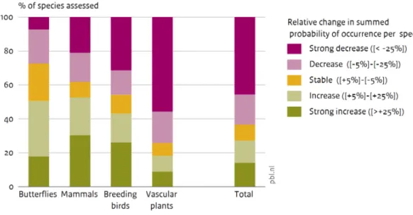
Species indicator

The first indicator presents the fraction of assessed species which show a (strong) decrease or increase (in summed probability of occurrence), when comparing a reference year with a target year, given a scenario (Figure 3.1). These results can be considered as a proxy for the relative change in species occurrence.

Figure 3.1. Indicator of the relative change in summed probability of occurrence for all assessed species and per taxonomic group.

Ecosystem indicator

The second type of indicator concerns the ecosystem level. Figure 3.2 shows the change in ecosystem quality within forests, agriculture, urban area and open vegetation and the area it concerns. This indicator type can also be visualised in map (Figure 3.3).

(27)

Figure 3.2. Indicator of relative change in summed probability of occurrence for shrubs and open vegetation, forests, agriculture and urban area.

(28)

3.3 Modelled effect of climate change

The effect of climate change on European protected species is modelled using BioScore 2.0. The model has been used to assess the effect of the trend scenario for 2050 and a scenario directed towards achieving the Paris Agreement on Climate Change to keep temperature rise well below 2 degrees Celsius until 2100 – instead of 4 °C in 2100, or 2 °C in 2050 (Figure 3.4). A considerable share of the species assessed is strongly negatively impacted by the expected changes in climate. Achieving the objective of the Paris Agreement on climate change – to limit global temperature increase to well below 2 °C, instead of 4 °C by 2100 or 2 °C by 2050, as was assumed in the Trend scenario – decreases the strong negative impact for many species.

Figure 3.4: A sensitivity analysis has been carried out of the effects of achieving the Paris Agreement on Climate Change to keep temperature rise well below 2 degrees Celsius until 2100 – instead of 4 °C in 2100, or 2 °C in 2050, also see Van Zeijts et al. (forthcoming).