Population models for time-varying pesticide exposure

* Corresponding author. E-mail: TP.Traas@rivm.nl Expertise Centre for Substances

RIVM report 601516015/2007

Population models for time-varying pesticide exposure T. Jager, F.M.W. de Jong, T.P. Traas

This investigation has been performed by order and for the account of the Board of Directors of the National Institute for Public Health and the Environment, within the framework of project 601516, Kennislacunes risicobeoordeling

Het rapport in het kort

Populatiemodellen voor de effecten van bestrijdingsmiddelen

Het RIVM heeft een nieuw model ontwikkeld dat de effecten van in de tijd variërende blootstelling aan bestrijdingsmiddelen op de planten- en dierenpopulatie in oppervlaktewater kan voorspellen.

Voordat een bestrijdingmiddel op de markt komt, wordt gekeken naar het zogenaamde milieurisico van dit middel. Het milieurisico wordt bepaald door het vergelijken van de mate van blootstelling van planten en dieren aan het bestrijdingsmiddel met de verwachte gevoeligheid van planten en dieren voor het betreffende bestrijdingsmiddel.

Het ontwikkelde model bestaat uit een combinatie van een model dat de ontwikkeling van de populatie beschrijft en een model dat een variabele mate van blootstelling combineert met de effecten daarvan op de groei en overleving van planten en dieren. Deze combinatie biedt een oplossing voor het praktische probleem dat in het laboratorium de planten en dieren niet in alle leeftijden en bij alle mate van blootstellingen kunnen worden onderzocht. Naast de werking van het model wordt in het rapport ook aangegeven welke gegevens nodig zijn om het model te kunnen gebruiken.

Trefwoorden:

Abstract

Population models for time-varying pesticide exposure

A model has recently been developed at RIVM to predict the effects of variable exposure to pesticides of plant and animal populations in surface water.

Before a pesticide is placed on the market, the environmental risk of the substance has to be assessed. This risk is estimated by comparing the exposure of plants and animals to the pesticide with the expected sensitivity of these plants and animals to the particular pesticide. The model presented here consists of a combination of two models: one describing the development of a population and one combining the variable exposure with growth and survival of plants and animals. This combination offers a practical solution to the problem that it is not possible to study all stages and all exposure regimes in the laboratory. Separate from the model itself, indications are given about the data needed to use the model.

Key words:

Contents

2 Description of the model 11

3 Discussion 26

4 Conclusions and recommendations 29

References 30

Appendix 1 Matlab scripts 32

Summary

In pesticide risk assessment the risks for aquatic organism are estimated by comparing the predicted environmental concentration (PEC) with the predicted effects on these organisms. A large number of factors determines the exposure of organisms, such as drift during spraying of plant protection products, run-off from the soil after rain and drainage from the soil. Apart from these routes, exposure is determined by the compound properties, such as the disappearance time, solubility in water and ability to bind to soil particles and organic matter. In addition, the way and the moment of application, and the number of applications are important for the exposure of aquatic organisms. All these elements can result in a variable exposure pattern. In the registration procedure, exposure is estimated with the use of sophisticated models that are able to predict such a variable exposure pattern.

In the first tier of the risk assessment, the effects on organisms in surface water are estimated in laboratory experiments. In these tests, organisms of a certain life stage are exposed to an acute dose, and then the effects on growth and survival are measured. In order to estimate the effects on the long term, the organisms are exposed to chronic concentrations, and apart from effects on growth and survival, effects on reproduction are examined, depending on the species.

The predicted exposure is then compared to the predicted toxicity, and when certain trigger values are exceeded, further data should be provided before a compound can be approved. For the estimation of the exposure, the variation in the parameters mentioned above can be incorporated into the models with relatively little extra effort. For estimating the effect, however, a separate test should be conducted for each exposure regime. In practice, it is impossible to study the effect on all life stages and possible combination in toxicity experiments.

To solve these problems in risk assessment, a model has been developed that is able to predict the effects of a variable exposure to populations of aquatic organisms. The model that is described in this report combines a description of the development of a population with a time varying exposure, leading to a prediction of time varying effects on growth, reproduction and survival.

For the population model, a technique [‘escalator boxcar train’, EBT] has been chosen, that has the possibility to follow the development of cohorts of individuals over continuous time. The time intervals are chosen so that the cohorts can be characterized by an average size of the individuals. Thus, each cohort can be characterized by a single set of state variables. The Dynamic Energy Budget model for chemicals [DEBtox] is able to combine a variable exposure with variable effects. This model takes into account the assimilation of food in the reserves of an organism, the energy needed to maintain the organism, for growth and reproduction and the risks for the embryo and the impact of toxic substances on these aspects.

All these aspects are dependent on the size and the life stage of the organism, but for instance also on the food availability.

Combining both models offers the opportunity to calculate the effects of single and variable exposure on populations of aquatic organisms. In the report an example is elaborated, showing that a population is able to recover after a single dose, but not after repeated dosing. Until now, modeling methods were not sufficiently practical to predict these kinds of effects. In another example it is shown that the availability of food is a determining factor for the effects of a toxic substance on population development.

In the case of Daphnia, the data needed to use the model are available from the standard reproduction test. The intermediate measurements of survival and reproduction as prescribed by the protocol are however needed and should be included in the study report. Repeated measurements of the length would increase the reliability of the DEBtox model. For algae the data from standard tests can be used directly. For both tests it is recommended that a recovery period after exposure, preferably in an uncontaminated medium, is followed and reported so they can be used for the model.

The fish data as present in the standard dossiers are not sufficient to apply the model.

It is concluded that the model can predict the influence of toxic substances on populations of invertebrates, and after extension of the model also for algae and possibly plants. Especially in the case of repeated application of compounds, the model can enhance insight into the effects on population development. These effects would not come to light with the currently used methods. If the model predicts population effects (based on laboratory studies) above an agreed threshold level, targeted population experiments with the relevant exposure pattern could be conducted to elucidate the cause for concern.

Samenvatting

Bij de toelating van bestrijdingsmiddelen wordt het milieurisico voor organismen in het oppervlaktewater geschat door het vergelijken van de verwachte blootstelling met de verwachte effecten op die organismen.

De blootstelling van de organismen wordt bepaald door veel verschillende factoren, zoals bij voorbeeld de verschillende routes waarmee het bestrijdingsmiddel in het milieu terecht kan komen (onder andere verwaaiing tijdens de bespuiting, afspoeling van de bodem na een regenbui en uitspoeling uit de bodem). Daarnaast wordt de blootstelling ook bepaald door de eigenschappen van het middel, bijvoorbeeld de afbraaksnelheid van het middel, de oplosbaarheid in water en de bindingscapaciteit aan bodemdeeltjes en organische stoffen. Verder spelen ook de wijze waarop het middel wordt toegediend, het moment van toediening en het aantal toedieningen een belangrijke rol. Al deze factoren leiden ertoe dat de blootstelling in de praktijk een grillig patroon kan vertonen. Bij de toelating wordt de blootstelling geschat met geavanceerde modellen, die een variabele blootstelling kunnen voorspellen.

De effecten op organismen in het milieu wordt in eerste instantie geschat door proeven in het laboratorium. Bij deze proeven wordt een bepaald levensstadium van een organisme blootgesteld aan een éénmalige dosering, waarna de effecten (in het algemeen overleving of groei, afhankelijk van het organisme) worden gevolgd. Om effecten op lange termijn in te schatten, worden de organismen langdurig blootgesteld, waarbij naast effecten op groei en overleving ook effecten op reproductie worden onderzocht, ook hier afhankelijk van het organisme.

De voorspelde blootstelling wordt vervolgens vergeleken met de voorspelde toxiciteit, en als bepaalde waarden worden overschreden is nader onderzoek noodzakelijk voordat het middel kan worden toegelaten.

Bij berekening van de blootstelling kunnen met relatief weinig extra inspanning de gevolgen van variatie in de parameters worden doorgerekend. Voor het inschatten van de effecten zou dit betekenen dat er voor elk blootstellingspatroon een aparte toets moet worden uitgevoerd. Daarnaast speelt nog het probleem dat niet alle mogelijke levensstadia en combinaties daarvan kunnen worden onderzocht. In de praktijk is dit niet mogelijk.

Om aan een deel van deze problemen het hoofd te kunnen bieden is een model ontwikkeld waarmee de effecten van variabele blootstelling op populaties van aquatische organismen kunnen worden voorspeld.

Het ontwikkelde model bestaat in principe uit een combinatie van een model dat de ontwikkeling van een populatie beschrijft, met een model dat in staat is een over de tijd variërende blootstelling te combineren met over de tijd variërende effecten op groei, reproductie en overleving.

Voor het model dat de populatie beschrijft, is gekozen voor een techniek [‘escalator boxcar train’, EBT], die de mogelijkheid geeft de individuen doorlopend over de tijd te volgen. Hierbij worden tijdsintervallen zo gekozen dat de cohorten kunnen worden gekarakteriseerd door een gemiddelde omvang van de individuen. De individuen in de cohorten zijn hierdoor gekarakteriseerd door een enkele set van variabelen.

Een geschikt model dat in staat is de variabele blootstelling te combineren met de variabele effecten is het Dynamic Energy Budget model voor chemische stoffen [DEB]. Dit model bekijkt de volgende aspecten: de assimilatie van voedsel in de reserves van een organisme, de energie die nodig is om het organisme te onderhouden, om te groeien, voor de reproductie en de risico’s voor het embryo en de invloed van toxische stoffen op elk van deze aspecten. Al deze aspecten zijn afhankelijk van de omvang en het levensstadium van het betreffende organisme, maar bijvoorbeeld ook van het beschikbare voedsel.

Door het combineren van beide submodellen kunnen de effecten van een enkele èn een variabele blootstelling op een populatie worden weergegeven. In het rapport wordt een voorbeeld uitgewerkt waaruit blijkt dat een populatie zich na een enkelvoudige toediening aan een bestrijdingsmiddel nog hersteld, maar na een herhaalde toediening hiertoe niet in staat was. Met technieken die tot nu toe gebruikt werden, was het niet mogelijk een dergelijke voorspelling te doen. Daarnaast wordt een voorbeeld gegeven waaruit blijkt dat de voedselbeschikbaarheid een grote invloed heeft op de effecten van een toxische stof op de populatieontwikkeling.

De gegevens die nodig zijn om het model te gebruiken worden voor Daphnia in de standaard reproductie test al gegenereerd. Wel is hiervoor nodig dat de tussentijdse metingen van reproductie en overleving, die in het protocol staan, ook daadwerkelijk beschikbaar zijn. Voor de lengtemetingen zou de betrouwbaarheid van de voorspellingen van het DEBtox model sterk toenemen als hier ook op meerdere data zou worden gemeten. Voor algen kunnen de gegevens uit de standaardtesten direct worden gebruikt. Voor beide testen is het aan te bevelen dat ook een herstelperiode na een blootstelling wordt gevolgd, bij voorkeur in een niet gecontamineerd medium.

Voor vissen zijn de gegevens die in de standaardtoetsen worden verzameld niet voldoende om het model te kunnen toepassen.

Geconcludeerd wordt dat het model een belangrijke bijdrage kan leveren voor wat betreft de invloed van toxische stoffen op populaties van evertebraten, en na modeluitbreiding ook voor algen en planten. Vooral in het geval van herhaalde toediening van toxische stoffen kan het model inzicht verschaffen van het effect op de populatieontwikkeling. Deze effecten zouden met de bestaande methoden niet aan het licht komen. De resultaten van het model kunnen dan bijvoorbeeld de aanleiding vormen voor het uitvoeren van een gericht experiment met populaties van organismen gecombineerd met het verwachtte blootstellingspatroon.

1 Introduction

1.1 Background

Ecotoxicological risk assessment of pesticides in Europe is based on a tiered approach. The first step in the aquatic hazard assessment of pesticides in the EU (‘tier 1’) is based on a procedure (EC Directive 91/414/EEC), where the minimum data requirements are acute and chronic single species toxicity studies for at least an algal species, a Daphnia and a fish, and a bioconcentration factor (BCF) for fish when compounds are bioaccumulative. The data requirements and the guidelines used for the first tier assessment are summarised in Annex 2. The toxicity data for aquatic organisms are used to generate a toxicity-to-exposure ratio (TER). If the TER for acute toxicity:exposure is < 100, or chronic toxicity:exposure < 10, then further evaluation is needed. When these trigger values are exceeded, no authorization shall be granted, ‘unless it is clearly established through an appropriate risk assessment that

under field conditions no unacceptable impact on the viability of exposed species occurs - directly or indirectly - after use of the plant protection product according to the proposed conditions of use.’ Such an appropriate risk assessment is commonly referred to as higher tier

risk assessment.

Pesticides can fail to pass the first tier when substantial uncertainty about risks exists, e.g. about the effects on non-target species that resemble the target species. In this case, higher tier risk assessment is required. Higher tier tests should provide information to assess whether or not adverse effects can be expected in the field as a result of the use of the pesticide of concern according to Good Agricultural Practice and if so, what the duration and magnitude of adverse impacts is. The design and scale of a test for a specific chemical depends on the focus of the problem and the physical-chemical and toxicological properties of the substance. It is clear that the higher tier tests should provide a focus on the issues of concern identified in earlier tiers of the risk assessment, e.g. persistence, dispersion in (adjacent) water bodies, transfer to other compartments, bioaccumulation, and possible direct or indirect effects. The Higher tier Aquatic Risk Assessment for Pesticides (HARAP) workshop (Campbell et al., 1999) examined different types of higher tier studies and developed guidance on how to apply these methods. Intermediate methods between laboratory and field tests may contribute to a more (cost) effective higher tier risk assessment. This set of tools can be used to specifically address the uncertainty about a certain pesticide, depending on the areas of concern that were identified earlier. Additional single-species tests, population recovery studies, indoor microcosm experiments, outdoor micro/mesocosm tests, or a combination of these may reduce the uncertainty. By choosing an appropriate test, the higher tier risk assessment is tailored to the problem identified without necessarily resorting to a complex, expensive field test, or the full set of tools. Also further effect modeling fits in this approach (Boxall et al., 2002).

1.2 Problem definition

Organisms in the laboratory tests are exposed for a limited time to constant concentrations, whereas exposure in the field may be pulsed (especially for plant protection products), or otherwise varying in time (e.g. due to degradation or to different exposure routes, e.g. drift or run-off). Fate models are becoming more and more complex and complete, including different routes and scale levels (see e.g. FOCUS, 2001, 2006), resulting in complex exposure scenarios. Furthermore, standard toxicity tests on a single cohort in the laboratory may not accurately represent how a population in the field is affected, and how it can recover after the toxic insult.

Therefore, there is a clear need for modeling approaches that are able to translate the effects observed in laboratory tests to the populations in the relevant (time-varying) field situation. In this report it is worked out how existing models can be combined to support the risk assessment process for plant protection products.

In Chapter 2 the proposed model is described, including some examples. In Chapter 3 the model, the data requirements and the implementation are discussed and in Chapter 4 the conclusions and the recommendations are given.

2 Description of the model

Predicting the population effects for organisms such as daphnids and fish requires structured population models. A structured population is one where the individuals differ in one or more properties which describe the life cycle (the so-called i-states). In contrast, unstructured population models assume that all individuals are equal (e.g. in a log-logistic population growth model). For organisms that grow little over their lifetime (such as single-celled algae), unstructured models may suffice, but for other organisms we need to account for size and/or age differences. Organisms of different size respond differently to a toxic effect (e.g. because size affects the toxicokinetics), and therefore have to be treated differently.

Matrix models

Classical demographic modeling is based on the life table: specifying the age-specific survival and reproduction in matrix form (also known as the Leslie matrix). The i-state is age. The matrix can consequently be used to predict the changes in the population over a discrete time step (the projection interval). For each time step, the organisms can move to the next age class with probability Pi, or die with probability (1-Pi) (an organism cannot stay in the same class).

At a certain age, the organisms reproduce at a certain rate (in the example below: F3 in class 3 and F4 in class 4). The parameters P and F are called the ‘vital rates’.

1

2

3

4

F

F

P

P

P

The projection matrix is given by A, and can be used to predict population size (given in the vector n) for the next time step.

) ( ) 1 ( 0 0 0 0 0 0 0 0 0 0 0 3 2 1 4 3 t t P P P F F An n A = + ⎟⎟ ⎟ ⎟ ⎟ ⎠ ⎞ ⎜⎜ ⎜ ⎜ ⎜ ⎝ ⎛ =

In a matrix model, the states are discrete as well as the projection interval (in this case, the projection interval equals the distance between the i-states).

This approach assumes that ‘age’ is the appropriate factor that determines the survival and reproduction rates. This is particularly useful for species that are characterized as ‘demand systems’ (Kooijman, 2000): these organisms require a certain amount of energy input within narrow ranges to develop into adults and reproduce. They do not have the flexibility to deal with low food levels (they simply die), and as a result, age will be a good descriptor of an organism’s body size and reproduction rate. Mammals and birds belong to this category. In contrast, invertebrates and ectothermic vertebrates (e.g. fish) can generally be considered ‘supply systems’; it is not unusual for two individuals of the same age to show extreme differences in body size, depending on their feeding history. Age-structured modeling is therefore not the first choice for these organisms. Body size is probably a better descriptor of the individual for demographic purposes (e.g., reproduction usually starts at a fixed body size, not at a fixed age).

As alternative, stage-structured models can be developed (using size or life stage as the i-state). Each projection interval, an individual has the possibility to stay in the same size class (P) or grow to the next one (G). Clearly, P and G are closely related; when there is no mortality P = 1 – G, and they are governed by the growth rate.

1

2

3

4

F

F

G

G

G

P

P

P

P

The projection matrix is given by:

) ( ) 1 ( 0 0 0 0 0 0 0 4 3 3 2 2 1 3 3 1 t t P G P G P G F F P An n A = + ⎟⎟ ⎟ ⎟ ⎟ ⎠ ⎞ ⎜⎜ ⎜ ⎜ ⎜ ⎝ ⎛ =

Again, the matrix projects over discrete time steps, and the i-state (e.g. body size) is also discrete. This is clearly more complicated than the age-structured model, and includes more parameters. In the age-structured model, it was clear that all individuals move to the next age class or die. For the stage-structured ones, the transition to the next stage will be probabilistic and depend on the growth rate. The calculation of the vital rates is not so trivial, and can

easily become quite complicated (see Caswell, 2001). Nevertheless, this calculation offers many opportunities to simulate population behaviour in time-varying environments.

Limitations of matrix models

The use of matrix models has several limitations. Firstly, both time and the i-state are taken in discrete steps (the projection interval and the discrete size or age classes), whereas they are continuous in real life. The consequences of this problem can be decreased by increasing the number of stages, and decreasing the length of the projection interval. This discretization, however, also implies that some tricks have to be performed to fit continuous processes (mortality and reproduction) into the parameters P, G and F (see Caswell, 2001, but also Klok and De Roos, 1996). For the purpose of time-varying environmental concentrations we run into other problems. We need to consider the toxicokinetics of the compound, because the internal concentration is causing the effect. However, individuals in the matrix model are not identifiable as organisms jump from one discrete stage to the next. Thus, the only consistent option would be to assume the same toxicokinetics for all individuals in the population (just as a time-varying external stressor such as temperature). This assumption has two shortcomings. Firstly, toxicokinetics are determined by body size because the kinetics depend on the surface:volume ratio of the organism (large individuals take longer to reach steady-state than small ones) and because of growth dilution. For example, small organisms often appear to be more vulnerable in short-duration experiments, because they take up chemicals much faster (especially when they are not fed during the experiment, and thus cannot dilute the internal concentration by growing). The second problem occurs when new organisms are born in the exposure period: in the matrix model, they immediately take on the internal concentration of all other individuals. This may be realistic when chemicals are transferred from the mother to the offspring (see e.g. Heiden et al., 2005). In summary, the stage-structured model involves some crude simplifications that may limit its applicability to time-varying exposure scenarios.

Klok and De Roos (1996) presented a matrix population model (stage structured) for the effects of copper on the earthworm Lumbricus rubellus. These authors do not have to deal with the toxicokinetics problem, as they stick to constant environmental concentrations, and ignore toxicokinetics altogether. This approach seems quite realistic for long-term exposure to constant concentrations, as is the case for earthworms exposed to copper in the field. However, if the only purpose is to predict population growth rates under constant environmental conditions, a matrix model is the wrong method to use. It is far easier and more accurate to directly apply the Euler-Lotka equation to the (splined) data for survival and reproduction throughout the life cycle (see Kooijman and Bedaux, 1996b; Caswell, 2001; Jager et al., 2004). This probably means that the bulk of the matrix modeling in ecotoxicology is actually unnecessary! Klok and De Roos also discuss the effects of copper on the stable stage distribution (how the animals are distributed over the different stages), which does require matrix models. However, matrix models only provide a real advantage when the environment is changing (e.g. food level or temperature). In case of time-varying concentrations of the toxicant, the matrix models have the limitation that only one state is followed (e.g. stage or size), so the toxicokinetics cannot be accurately included in the model.

Continuous time

The method to include more than one state variable, involving the least simplifications, would be to model all individuals in continuous time with a separate set of equations (partial differential equations), but this will require a large amount of computer resources. As a compromise, De Roos and co-workers (De Roos et al., 1992) presented the ‘escalator boxcar train’ (EBT) technique. The EBT follows the development of cohorts of individuals over continuous time. Reproduction is continuous, so the members of the cohort were not born at the same time. However, if we consider the individuals born over some small time interval, we can characterize them by their average size. Thus, we can characterize each cohort by a single set of state variables (i.e. all individuals within a cohort have the same body size and internal concentration). Instead of following all individuals, we now only have to follow a limited number of ‘characteristic’ individuals over continuous time. However, we also have to deal with the boundary cohort; the cohort collecting the newborn individuals. The reproduction over a certain time interval is collected into a new cohort, which is closed at the end of the interval, when a new boundary cohort is created. This process would lead to a steady increase of the number of cohorts in simulation time. However, a cohort disappears when all the individuals in that cohort have died (or when there are so few individuals left, that we can safely ignore their contribution to the population), and when ageing cohorts become very similar, they may be lumped. The number of cohorts that need to be followed depends on the time interval during which we fill up the boundary cohort; the shorter this interval the more detail we add at the cost of increased number of calculations. The advantage of this approach is that we can calculate the fate of each cohort in continuous time, avoiding the errors made by introducing discrete projection intervals. This also makes it easy to introduce additional i-states (e.g. internal concentration of toxicants, or oxidative damage to include the ageing process, see Jager et al., 2004, or age). The simplification occurs through the collection of individuals born within a certain interval in a cohort, and giving them the same properties.

PDE (partial differential equation) models for toxicokinetics and toxicodynamics

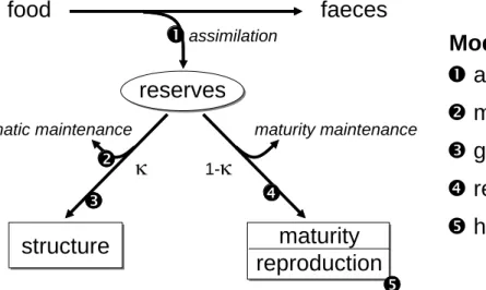
To apply the EBT technique to the time-varying influence of toxic compounds, we need models for toxicokinetics (the time course of internal concentrations) and toxicodynamics (the link between the time course of internal concentrations and the time course of effects). The only available approach that is able to link time-varying concentrations in the environment to time-varying effects on growth, reproduction and survival is the DEBtox method (Kooijman and Bedaux, 1996a; Kooijman and Bedaux, 1996b). The DEBtox method is based on the theory of dynamic energy budgets (DEB, Kooijman, 2000; Nisbet et al., 2000; Kooijman, 2001), which provides simple rules for the metabolic organization of organisms. The basic DEB scheme is shown in Figure 1, including the points where chemicals may influence resource allocation. A thorough discussion of the DEB and DEBtox concepts is outside the scope of this paper; the reader is referred to (Kooijman and Bedaux, 1996b; Kooijman, 2001; Jager et al., 2004; Jager et al., 2006).

food

faeces

reserves

structure

maturity

reproduction

κ

κ

n

n

n assimilation

o

o

o maintenance costs

p

p

p growth costs

q

q

q reproduction costs

r

r

r hazard to embryo

Modes of action

Figure 1. Schematic representation of a Dynamic Energy Budget model. Numbers represent some of the positions where toxicants may affect resource allocation.

The DEBtox approach results in a limited number of partial differential equations. A number of scalings is applied to simplify the mathematics (but not the interpretation, unfortunately). Effects relate to internal concentrations, so the first step is a toxicokinetics model (here, a one compartment model, accounting for changes in body size) to go from external concentrations (ce) to body residues. However, the internal concentrations are not usually determined in

toxicity tests. Therefore, the scaled internal concentration (cq) is introduced. The internal

concentration is scaled with the unknown BCF, to yield the variable cq, which is directly

proportional to the internal concentration, but has the dimensions of an external concentration (in equilibrium, cq equals ce). The scaled internal concentration is a function of ce and scaled

body size (l, scaled to the maximum size in the control at abundant food).

⎟ ⎠ ⎞ ⎜ ⎝ ⎛ ₊ − = dt dl l l k c l k c dt dc _e q e e q 3 _[1]

The only unknown parameter (if we know the external concentration and the body size) in this equation is the elimination rate (ke). This is a simple one-compartment model, but accounting

for the effect of body size on the exchange kinetics (reflecting changes in the surface:volume ratio) and dilution of body residues. Note that ke is the elimination rate at l=1, which is for a

fully grown individual at abundant food. Even without measured body residues, the toxic effects in time usually provide enough information to estimate a single toxicokinetic parameter from the data. Also note that for this model, the external concentration ce does not

need to be constant. However, to estimate effects parameters from toxicity data it helps when the exact pattern of ce in time is known.

To provide an impression of the degree of complexity of DEBtox, below the equations for the mode of action ‘effects on assimilation’ are given. More detail is given in Kooijman and Bedaux (1996b), but it must be noted that the derivation of these equations from the full DEB theory is currently being re-evaluated, which will lead to some changes in formulation.

To include the effect of toxicants on the process of assimilation, a stress factor is introduced:

(

)

Stress is zero when cq is below the no-effect concentration for assimilation, c0A. Above the no-effect concentration, the stress increases linearly in the internal concentration. This is a very simple model for the internal dose response, which works well in practice. Usually, the available toxicity data are not detailed enough to fit more elaborate dose-response models. The scaled length (l) in time is given by the following differential equation:

(

)

[

]

Where rB is known as the von Bertalanffy growth rate constant, and f is the relative ingestion

rate (which is 1 at abundant food, and decreases with food limitation). The reproduction rate (in offspring per time unit) is given by the following equation:

(

)

Where Rm is the maximum rate, lp is the scaled length at puberty (first investment in

offspring), and g is the energy investment ratio (the ratio of the volume-specific costs for growth to the fraction of the reserve density allocated to maintenance and growth). The value for g is usually difficult to obtain from toxicity data at one food level alone. A value of 1 serves as a good initial guess (Kooijman and Bedaux, 1996b).

Mortality is treated as a chance process: above the NEC, the internal concentration increases the probability to die (see Bedaux and Kooijman, 1994). It appears that a stochastic model for mortality is more realistic than assuming a distribution of tolerances in the test population (Kooijman, 1996; Newman and McCloskey, 2000). The statistical technique to deal with probabilistic events in time is known as ‘survival analysis’, which works through the specification of a hazard rate. The hazard rate (h) is zero (or a low background value h0) when cq is below the NEC (c0s). Above the NEC, the hazard is taken proportional to the concentration above the NEC:

(

)

max c c h

b

h= _q − _s + [5]

The proportionality constant b is known as the killing rate. The fraction surviving individuals over time is than calculated by integrating the hazard rate over time:

⎟⎟ ⎠ ⎞ ⎜⎜ ⎝ ⎛ − =

∫

Note that the relative ingestion rate is included as a parameter in the equations for body size and reproduction. The effects of food limitation can thus easily be assessed (Jager et al., 2005) or simulated (assuming that the intrinsic sensitivity does not change), as demonstrated earlier (Jager et al., 2004; Alda Álvarez et al., 2005; Jager et al., 2006). Generally, the relative ingestion rate will not be directly proportional to the food concentration, but they will be linked through the functional response (such as the Holling type responses).

With these equations, the DEBtox model is specified. Because a toxicokinetic model is used (Eq. 1), a time-varying external concentration is translated into a time-varying (scaled) internal concentration. The effects models simply translate the internal concentrations to effects in time. This calculation is representative on the precondition that effects are directly related to the actual internal concentration; that they are in fact fully reversible. A decrease in the internal concentration to zero should lead to a return to the performance level of the unexposed situation. This may not be valid for all chemicals; for example, it is conceivable that some chemicals induce permanent damage to the reproductive system, making it impossible for the organism to produce offspring, even when the chemical is fully eliminated from the body.

These equations make some simplifications of the full DEB theory. Firstly, the reserve dynamics is simplified by assuming that the reserves are always in equilibrium with the food supply. This works well, as long as there are no rapid changes in food level or assimilation. Secondly, a specific value for the maturity maintenance (see Figure 1) is taken, which leads to a constant size at first reproduction (lp). A constant size at puberty is often observed, but not

always (Alda Álvarez et al., 2005). Nevertheless, a different value for the maturity maintenance would require a more complicated model (not in terms of parameters, but in terms of the number of differential equations).

Combining DEBtox with population models

The DEBtox method is one of the few available approaches to predict effects on survival, growth and reproduction in time, also under time-varying conditions (toxicant levels as well as other parameters such as food). This was nicely demonstrated in the paper by Pieters et al. (2006). Basically, there are two options for combining DEBtox with population models:

1. use an size-structured model assuming that the toxicokinetics is the same for all animals (and that offspring has the same body burden as their mother)

2. use an EBT approach, following cohorts of DEB individuals, allowing for more realistic modeling of individuals.

Combination of DEBtox with age-structured model has been done (Lopes et al., 2005), but is not generally advisable (see earlier comments). Age is not a good descriptor of the behaviour of ectotherms, one loses information due to the discretization in stages, and cannot properly include toxicokinetics. The simplified DEBtox model as presented in Kooijman and Metz (1984) has been combined with a stage-structured model (Klok and De Roos, 1996), as well

as with an EBT approach (Baveco and De Roos, 1996). However, in both cases, the toxicokinetics have been ignored completely.

Size-structuring and DEBtox

For toxicokinetics, we have to use a simple model, ignoring body growth altogether (both effects on the rate constant, as well as the effect on growth dilution). This implies that all individuals at time t have the same internal concentration (as well as the newborn juveniles):

(

)

e

q c e e

c = 1− − [7]

The cq can be used to calculate the stress function (Eq. 2) and the hazard rate (Eq. 5). For

every class i, we can define a characteristic individual with length Li as the average length in

the size class. The average growth rate is given by dLi/dt. Assume that the survival probability

in stage i (σi) is constant. The time spent in class i (Ti) is given by:

dt dL L T i i i / Δ = [8]

where ΔLi is the width of the size class i. The growth rate dLi/dt can be directly derived from

the DEBtox equation (Eq. 3), using the average length in the size class and the toxicant stress. Next, we define γi as the probability to grow from stage i to stage i + 1, given that the

organism survives in the projection interval. And σi as the probability of an individual in stage i to survive in the projection interval (see Caswell, 2001, page 160).

(

)

The survival probability follows from the hazard rate (hi). Assuming that the hazard rate is

constant within a class and within the projection interval:

t h i e i Δ − = σ [10]

Suppose that every individual spends a fixed time Ti in stage i and then graduates to stage i +

1. The probability of graduation is not constant, but depends on the age distribution within the stage. An approximate constant γi can be calculated by assuming that the age distribution

within the stage is constant (see Caswell, 2001, page 160-161).

1 1 − ⎟ ⎠ ⎞ ⎜ ⎝ ⎛ ⎟ ⎠ ⎞ ⎜ ⎝ ⎛ − ⎟ ⎠ ⎞ ⎜ ⎝ ⎛ = − i i i T i T i T i i λ σ λ σ λ σ γ [11]

where λ is the population multiplication rate (dominant eigenvalue). The γi can be estimated

with λ = 1, or iteratively (see Caswell, 2001, Page 164). The fertility of each class can be calculated, assuming a constant reproduction. The problem is that ni changes within the

projection interval. Furthermore, we have to consider the mortality of the offspring that are born in an interval. We could calculate a kind of averaged fertility (see Caswell, 2001,

page 171):

(

)

The first term is the probability of the offspring to survive half a projection interval (the average age of the offspring born). The mi is the average reproduction rate in stage i.

Following cohorts (EBT) and DEBtox

The option to follow cohorts instead of size-structuring leads to more realism, but also to a much simpler model. It is possible to directly use the DEBtox equations to describe the behaviour of the cohorts. A disadvantage is that you cannot estimate eigenvalues of the population matrix (because there is no such matrix), or use shortcuts to obtain sensitivities of eigenvalues for changes in vital rates. A simple version of such an analysis was programmed in MatLab (code is added as appendix to this memo). We first have to distinguish between two time intervals: the time over which the reproduction is collected in a new cohort (the ‘cohort width’ ΔT), and the time scale for calculation of the behaviour of the cohorts (Δt, which may also be done in continuous time). The number of cohorts to be followed thus depends on ΔT and the time it takes for a cohort to die out, and not on Δt. The behaviour of each cohort in time is described by the continuous DEBtox equations. For this example, they were calculated in small discrete steps using an Euler scheme (more elaborate ODE solvers could be used here). The produced juveniles over a certain cohort width (ΔT) are collected in a ‘cohort in creation’. Within a cohort, all individuals are equal, so we need to decide what a representative state is when a cohort is being created. We decided to take the individuals that are born at 0.5ΔT as representative. In other words, the cohort in creation starts to grow and accumulate toxicants at half of the time interval over which it is created.

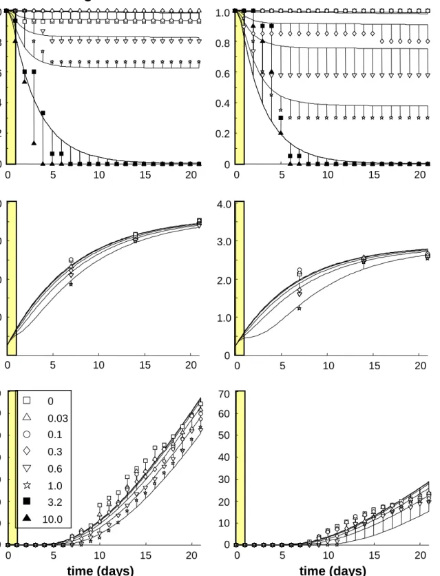
The model is parameterized using data for Daphnia, pulse exposed to the pyrethroid insecticide fenvalerate (Pieters et al., 2005), see Figure 2 and Table 1 (the DEBtox fit and parameter values are presented in Pieters et al., 2006). The experiments were performed at two food levels with the same parameters (apart from the relative ingestion rate f), indicating that the intrinsic sensitivity does not depend on food availability. From Figure 2, it is clear that mortality still continues after the exposure period (owing to the slow elimination kinetics of this compound). The pulse exposure leads to the delay in growth and reproduction, but the same final body size and the same reproduction rate (thus indicating reversibility of effects).

high food

low food

time (days) time (days)

bod y l e ngt h (m m) cumul a ti v e rep roduct io n fr ac ti on surv iv al 0 0.2 0.4 0.6 0.8 1.0 0 1.0 2.0 3.0 4.0 0 5 10 15 20 0 0.2 0.4 0.6 0.8 1.0 0 5 10 15 20 0 5 10 15 20 0 1.0 2.0 3.0 4.0 0 5 10 15 20 0 5 10 15 20 0 10 20 30 70 40 50 60 0 5 10 15 20 0 10 20 30 70 40 50 60 0 0.03 0.1 0.3 0.6 1.0 3.2 10.0

Figure 2. Data and simultaneous model fits for Daphnia magna pulse exposed (for the first 24 h as indicated by the coloured bar) to fenvalerate at two food levels. Legend indicates the nominal exposure concentrations (fits were based on measured pattern of disappearance within this exposure day).

Table 1. Parameter estimates of the model fits in Figure 2, with likelihood-based 95% confidence intervals given between brackets. Mode of action is a decrease in assimilation due to fenvalerate.

Description Symbol Unit High and low food

simultaneously Physiological parameters

Von Bertalanffy growth rate rB d-1 0.138 (0.132-0.143)

Initial length Lo mm 0.753 (n.e.)

Length at first reproduction Lp mm 2.38 (2.32-2.42)

Maximum length Lm mm 4.15 (4.12-4.18)

Maximum reproduction rate Rm juv/d 7.24 (6.90-7.53)

Scaled food density f - HF: 1.0 (n.e.)

LF: 0.818 (0.809-0.825) Toxicological parameters

Elimination rate ke d-1 2.37 (1.33-10.1) × 10-3

Blank hazard rate h0 d-1 0.665 (0.231-2.66) × 10-3 NEC for survival c0s μg/L 132 (49.2-228) × 10-6 NEC for assimilation c0a μg/L 0 (0-1.18 × 10-5) Tolerance concentration cT μg/L 5.39 (2.72-18.5) × 10-3

Killing rate b L (μgd)-1 _{74.4 (55.6-96.4)} Maximum water solubility - μg/L 0.524 (0.473-0.593)

Note that the maximum reproduction rate is quite low. The food level used as ‘high food’ is already limiting the organism’s development. Results from another study (see Jager et al., 2006) showed maximum reproduction rates for Daphnia of 38 juv/d, and a maximum length of 4.7 mm (although it is possible that a different length measure is used). Thus, care must be taken when using these results in a population model with higher food levels. Furthermore, the concentrations given in the legend of Figure 2 are the nominal exposure concentrations. The calculations make use of the most likely pattern of exposure in time: an exponential decrease over the 24-h exposure period, due to sorption to the glass walls (the pattern is based on a few measured concentrations, for details see Pieters et al., 2006). This nicely shows that it does not matter for the DEBtox estimation what pattern the external concentration follows in time, as long as the pattern is known.

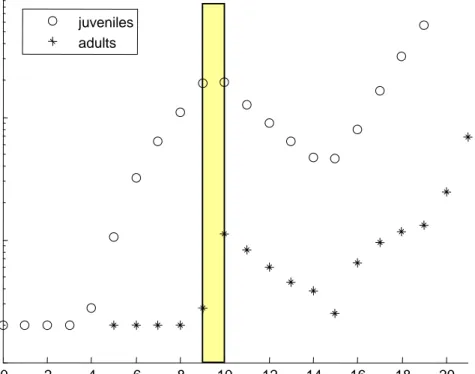
Using the specification in Table 1, a simplified version of the EBT calculation was parameterized for the population. Now it is possible to simulate the effect of a pulse exposure on the population (Figure 3). In this case a 1-day, 1 µg/L pulse is used (it should be noted that this is in fact above the water solubility for this compound). Initially, there is a lag in the population growth, because the simulations were started with juveniles. After some time, the population starts to grow exponentially, but the exposure to the insecticide knocks out a large part of the population. Even after the peak has subsided, the population still decreases because the compound is still present in the organisms’ body (as was also clearly seen in Figure 2). However, five days after the exposure, the exponential growth of the population is restored. If

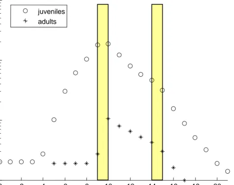
there is another pulse of the same magnitude after five days (Figure 4), this will lead to extinction of the population. For the model, it makes no difference what shape of the exposure concentration it is presented with. There is no limit to the number of peaks or the peak shapes. The toxicokinetic model (Eq. 1) simply translates the time-varying external concentration to a time-varying internal concentration, and links the effects to them.

0 2 4 6 8 10 12 14 16 18 20 101 102 103 104

time (days)

numbe

rs

Figure 3. Simulation of a Daphnia population, starting with 20 juveniles, exposed to a

24-h pulse of fenvalerate (constant exposure at 1 µg/L) at day nine. Note that the Y-axis is on log-scale.

0 2 4 6 8 10 12 14 16 18 20 101 102 103 104 juveniles adults juveniles adults

time (days)

numbe

rs

Figure 4. Simulation of a Daphnia population, starting with 20 juveniles, exposed to two 24-h pulse of fenvalerate (constant exposure at 1 µg/L) at day 9 and at day 14. Note that the Y-axis is on log-scale.

At this moment, the Daphnia population grows exponentially without toxicant stress, which is hardly realistic. The next step would be to include the algal food levels that decrease in time due to grazing, or a density dependent predation pressure to get a more realistic situation. Note that it will be quite important to know whether the population is limited by food availability or by predation. A toxicant affecting assimilation or maintenance will have a much larger effect on food-limited individuals than on individuals experiencing ad libitum food levels (as will be the case in predation-limited populations) (see Kooijman and Metz, 1984; Jager et al., 2004; Alda Álvarez et al., 2005). This shows that such modeling approaches require both toxicological and ecological information on the species of interest. The DEBtox method allows for a simple inclusion of food availability, as the relative ingestion rate (f, which relates directly to food levels) is a parameter in the model.

Inclusion of feeding

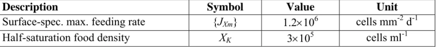
The feeding rate JX (e.g. algal cells/d for daphnids) is assumed to depend on the squared

length (Kooijman, 2000), and the level of food in the environment. Therefore, the maximum surface-specific feeding rate ({JXm} in cells/mm2/d) is a constant. The feeding rate relates to

the available food density by the functional response (usually a hyperbolic function, such as the Holling type II). To account for this relationship, we introduce the relative ingestion rate (f), which depends hyperbolically on the food density, and is known as the scaled functional response (note that L2 equals (l Lm)2).

2

} {J fL

J_X = _Xm [13]

with the relative ingestion rate given by:

K X X X f + = [14]

The food level (X) is given in cells/ml and so is the saturation density is XK. The total removal

of algae from the system is given by summing over all the cohorts (i) the products of the feeding rate (JXi) with the number of individuals in each cohort (Ni). If we consider a system

with a fixed number of algal cells (NX0) added daily (as is for example done by Liess et al.,

2006), we obtain the following relation for the number of algal cells within a day:

∑

The algal density X is NX divided by the volume of the test chamber.

Table 2. Parameters for the feeding module for Daphnia magna, taken from (Kooijman, 2000, page 331).

Description Symbol Value Unit

Surface-spec. max. feeding rate {JXm} 1.2×106 cells mm-2 d-1

Half-saturation food density XK 3×105 cells ml-1

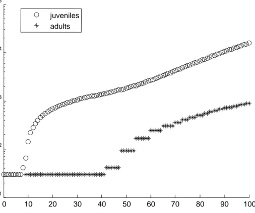
In the experiments of Liess et al. (2006), the volume of the container is 4.7 L, and the daily ration of algae leads to an initial food density of 1.63×105 _{cells/ml. This implies that each day} 7.66×108 _{cells are added. First, with this parameterization, the simulated daphnids were not} able to grow, so the daily food ration was increased by a factor of 5. When simulating this population for 100 days, the following result was obtained.

0 10 20 30 40 50 60 70 80 90 100 101 102 103 104 105 juveniles adults

time (days)

numbe

rs

Figure 5. Simulation of a Daphnia population, starting with 30 juveniles, without toxicants, but with a fixed daily food supply of algae. Note that the Y-axis is on log-scale.

This is clearly an unrealistic population behaviour: in practice, the juveniles will starve, leading to a depression of the total population size (as observed in Liess et al., 2006, and Kooijman, 2000, page 331). The reason for this artificial behaviour is due to the fact that our simulated Daphnids due not die as a result of food shortage. Instead they just stop growing and reproducing. However, at the start of each day, the get a fixed amount of food, which means that they can grow and reproduce a little bit, and wait for the next feeding moment. In practice, the juveniles will be the first ones to die as a result of food shortage, as they have very little buffering capacity (their energy reserves), compared to the adults. Thus, we will have to resort to the full DEB model, and include the reserve dynamics explicitly. The equations for the full DEB model under toxicant stress have been worked out in detail (Jager, in prep.), and although they require only a few additional parameters, they are much more calculation intensive.

3 Discussion

What is needed to produce population simulations?

To summarize, the following steps are needed to produce population predictions as presented for a new compound.

1. Generate or locate representative experimental data for the compound and the species of interest (see the section on data requirements).

2. Fit the DEBtox model to the data. The resulting parameter estimates (see Table 1) are used as input for the population model.

3. Define an exposure scenario; specify the exposure concentration in time, the initial population, predation pressure, and the dynamics of the food (e.g. the algae for

Daphnia).

4. Run the population model (see scripts in the appendix for a simple implementation of the EBT technique). The population calculations apply the same DEBtox equations, but follows cohorts of individuals over time.

Data requirements

The equations of the DEBtox model can be fit to toxicity data from (partial) life-cycle experiments. A proper data set constitutes measurement of survival, reproduction and body size over a good part of the life cycle; i.e. starting with eggs or juveniles, following their maturation, the start of reproduction, and at least a few reproductive events. This also implies that the test endpoints (growth, offspring and size) must be determined at several points in time, and not just at the end of the test. This sounds like an extensive test protocol, but in fact, the standard OECD Daphnia reproduction test comes very close already. The standard protocol prescribes that observations on survival and reproduction have to be made at least three times per week (although nothing is done with the intermediate data in the risk assessment). Further, the protocol advises to determine body size at the end of the experiment. Such a data set suffices to provide a fit of the model as specified above (see Jager et al., 2006), but for determining the most appropriate mode of action, more time points on growth would be advisable (see e.g. Pieters et al., 2006).

The same model approach is directly applicable to other (ectothermic) animals, such as fish. However, for fish, the standard chronic test follows only growth and survival of juveniles, and is therefore insufficient to assess population consequences. Unfortunately, partial life-cycle tests for fish are quite scarce. For algae, specific model formulations based on DEB theory have been developed (Kooijman et al., 1996) that can be used on standard OECD test data. The standard algae tests are already determining endpoints at the population level (population growth), and can directly be used in simple population models. However, for prediction of pulsed exposures, it may be useful to extend the test with a recovery period.

By default, DEBtox assumes that all toxic effects are fully reversible; the organism responds to the actual internal concentration. Therefore, as soon as the internal concentration decreases, the organisms’ performance will eventually return to the unpolluted situation. This was confirmed for Daphnia magna exposed to fenvalerate (Pieters et al., 2006), but may not be generally valid. Therefore, it would be preferable if testing considers the potential for recovery of the individuals. This could be done by prolonging a single test (21 days exposure of daphnids, followed by a recovery period of say 14 days in clean medium) or two tests (a test with constant exposure to get a good indication of the mode of action, and a test were juveniles are exposed to a pulse). The second option may be better for pesticide scenarios where high pulse doses are to be expected (a high exposure concentration may lead to irreversible damage, which may not occur at sub-lethal levels).

Acute survival tests have only very limited use for the prediction of population consequences. These tests could be made more relevant by including a recovery period. It is often observed that mortality continues even after exposure has ceased. This is often termed ‘latent mortality’ (Zhao and Newman, 2004), which in DEBtox terms would reflect that slow-eliminating chemicals may still be present in the body for some time after exposure stops, and exert a toxic effect (although this assumption is still in need of rigorous testing). Such an acute toxicity test can provide information on the mortality pattern after a pulse exposure, but says nothing about the recovery of other physiological processes, mainly growth and reproduction. In summary, to provide the proper input data for population models, experimental data should consist of partial life-cycle testing, following growth, reproduction and survival over time. To test the reversibility of toxic effects, the test should preferable be repeated with a pulse exposure (e.g. as done in Pieters et al., 2005). For algae and Daphnia, the standard (chronic) test protocols are already providing a lot of the required information. For Daphnia, it is advisable to measure growth at several points in time during the experiment. For fish, the standard tests do not provide useful information for population modeling. However, partial life-cycle testing following growth and reproduction in fish is probably not feasible or acceptable for the majority of compounds. Therefore, for fish, we need to find other ways to gain access to the required parameter values, e.g. through use of QSARs or in vitro techniques, which will require a serious amount of work.

Implementation in risk assessment

In pesticide risk assessment effect studies are conducted using an acute peak dose, or a chronic continue dose. Refinements are found in a more realistic composition of the community. On the fate site more and more realistic and complex exposure scenarios are being developed. This complexity is caused by different use patterns (repeated uses), different routes (e.g. drift, run-off, drainage) and in the highest tier even exposure patterns caused by the use on different parcels in an up-stream area. These predicted exposure patterns will seldom be directly comparable with the exposure in the test systems. Therefore models to predict the effects of time-varying exposure are inevitable. The method presented shows that this prediction is well possible, with a relatively limited extra effort in the standard tests.

For the practical implementation of the model a user-friendly interface will be needed. With the number of tools for effect assessment it will also be needed to clearly define when what tool is appropriate. For this aim a decision tree for aquatic effect assessment should be drafted.

The model will show the impact on the population development and recovery time of the species included. For use in risk assessment and as basis for regulatory decisions the protection goals need to be defined and translated to critical effect values: what magnitude and duration of a significant impact of exposure to a pesticide is acceptable?

4 Conclusions and recommendations

The DEBtox method, combined with an escalator-boxcar-train approach is most suitable to predict population consequences of time-varying exposures. This combination allows for a very flexible tool that can accommodate a range of different scenarios.

The currently available test data are in some cases unsuitable (acute mortality tests, fish growth) for population modeling, in other cases, they are already useful (algae population growth and Daphnia reproduction). Some slight modifications would greatly improve the usability of these tests (additionally testing a single pulse, and following growth of the Daphnids).

For fish, there is a need to develop methods to derive the model parameters in other ways (literature, QSARs, in vitro tests), as the required partial life-cycle test will not be feasible in most cases.

The presented approach of laboratory tests combined with population models fits very well into the HARAP approach in which specific methods are proposed for specific problems. Also field and mesocosm studies do not give an answer about the effects of a pulsed or irregular dose pattern. Furthermore, mesocosms studies are in general designed to trace community effects.

Recommendations

In order to show the applicability of the method it is recommended to work out a case study were all relevant data available in a pesticide dossier are taken into account. In this case study the attribution of the model should be illuminated. For the application of the model in daily risk-assessment a user friendly version should be developed. Further study is needed for an optimal implementation of the population calculations (the EBT technique).

Acknowledgements

We would like to thank Barry Pieters (UFZ, Dept. Chemical Ecotoxicology in Leipzig, Germany and University of Amsterdam, Dept. of Aquatic Ecology and Ecotoxicology in Amsterdam, The Netherlands) for providing the original data from his experiments.

References

Alda Álvarez O, Jager T, Kooijman SALM, Kammenga JE. 2005. Responses to stress of

Caenorhabditis elegans populations with different reproductive strategies. Funct Ecol 19:

656-664.

Baveco JM, De Roos AM. 1996. Assessing the impact of pesticides on lumbricid populations: an individual-based modeling approach. J Appl Ecol 33: 1451-1468.

Bedaux JJM, Kooijman SALM. 1994. Statistical analysis of bioassays based on hazard modeling. Environ Ecol Stat 1: 303-314.

Boxall ABA, Brown CD, Barrett KL. 2002. Higher tier laboratory methods for assessing the aquatic toxicity of pesticides. Pest Manag Sci 58: 637-648.

Campbell PJ, Arnold DJS, Brock TCM, Grandy NJ, Heger W, Heimbach F, Maund SJ, Streloke M (Eds.) 1999. Guidance document on higher tier aquatic risk assessment for pesticides

(HARAP), from the Europe/OECD/EC Workshop, Lacanau Océan, France, SETAC-Europe, Brussels, Belgium.

Caswell H. 2001. Matrix population models. Sunderland, MA, USA, Sinauer Associates.

Crane M, Newman MC. 2000. What level of effect is a no observed effect? Environ Toxicol Chem 19: 516-519.

De Roos AM, Diekmann O, Metz JAJ. 1992. Studying the dynamics of structured population models: a versatile technique and its application to Daphnia. The American Naturalist 139: 123-147. FOCUS. 2001. FOCUS Surface Water Scenarios in the EU Evaluation Process under 91/414/EEC.

Report of the FOCUS Working Group on Surface Water Scenarios, EC Document Reference SANCO/4802/2001-rev.2.

FOCUS. 2006. Guidance Document on Estimating Persistence and Degradation Kinetics from Environmental Fate Studies on Pesticides in EU Registration. Report of the FOCUS Work Group on Degradation Kinetics, EC Document Reference Sanco/10058/2005 version 2.0. Heiden TK, Hutz RJ, Carvan MJ. 2005. Accumulation, tissue distribution, and maternal transfer of

dietary 2,3,7,8,-tetrachlorodibenzo-p-dioxin: impacts on reproductive success of zebrafish. Toxicol Sci 87: 497-507.

Jager T, Crommentuijn T, Van Gestel CAM, Kooijman SALM. 2004. Simultaneous modeling of multiple endpoints in life-cycle toxicity tests. Environ Sci Technol 38: 2894-2900. Jager T, Alda Álvarez O, Kammenga JE, Kooijman SALM. 2005. Modeling nematode life cycles

using dynamic energy budgets. Funct Ecol 19: 136-144.

Jager T, Heugens EHW, Kooijman SALM. 2006. Making sense of ecotoxicological test results: towards application of process-based models. Ecotoxicology 15.

Klok C, De Roos AM. 1996. Population level consequences of toxicological influences on individual growth and reproduction in Lumbricus rubellus (Lumbricidae, Oligochaeta). Ecotox Environ Safe 33: 118-127.

Kooijman SALM, Metz JAJ. 1984. On the dynamics of chemically stressed populations: the deduction of population consequences from effects on individuals. Ecotox Environ Safe 8: 254-274. Kooijman SALM. 1996. An alternative for NOEC exists, but the standard model has to be abandoned

first. Oikos 75: 310-316.

Kooijman SALM, Hanstveit AO, Nyholm N. 1996. No-effect concentrations in algal growth inhibition tests. Water Res 30: 1625-1632.

Kooijman SALM, Bedaux JJM. 1996a. The analysis of aquatic toxicity data. Amsterdam, The Netherlands, VU University Press.

Kooijman SALM, Bedaux JJM. 1996b. Analysis of toxicity tests on Daphnia survival and reproduction. Water Res 30: 1711-1723.

Kooijman SALM. 2000. Dynamic energy and mass budgets in biological systems. Cambridge, UK, Cambridge University Press.

Kooijman SALM. 2001. Quantitative aspects of metabolic organization: a discussion of concepts. Phil Trans Royal Soc London B 356: 331-349.

Liess M, Pieters BJ, Duquesne S.. 2006. Long-term signal of population disturbance after pulse exposure to an insecticide: rapid recovery of abundance, persistent alteration of structure. Environ Toxicol Chem 25: 1326-1331.

Lopes C, Pery ARR, Chaumot A, Charles S. 2005. Ecotoxicology and population dynamics: using DEBtox models in a Leslie modelling approach. Ecol Model 188: 30-40.

Newman MC, McCloskey JT. 2000. The individual tolerance concept is not the sole explanation for the probit dose-effect model. Environ Toxicol Chem 19: 520-526.

Nisbet RM, Muller EB, Lika K, Kooijman SALM. 2000. From molecules to ecosystems through dynamic energy budget models. J Anim Ecol 69: 913-926.

Pieters BJ, Paschke A, Reynaldi S, Kraak MHS, Admiraal W, Liess M. 2005. Influence of food limitation on the effects of fenvalerate pulse exposure on the life history and population growth rate of Daphnia magna. Environ Toxicol Chem 24: 2254-2259.

Pieters BJ, Jager T, Kraak MHS, Admiraal W. 2006. Modeling responses of Daphnia magna to pesticide pulse exposure under varying food conditions: intrinsic versus apparent sensitivity. Ecotoxicology, on line: DOI 10.1007/s10646-006-0100-6

Zhao Y, Newman MC. 2004. Shortcomings of the laboratory-derived median lethal concentration for predicting mortality in field populations: exposure duration and latent mortality. Environ Toxicol Chem 23: 2147-2153.

Appendix 1 Matlab scripts

% By: Tjalling Jager (RIVM/LER) % Date: Mar-May 2006

%

% This script demonstrates how DEBtox can be combined with a simple

% Escalator Boxcar Train method to simulate the response of a population to % a toxicant stress.

clear all

dt = 0.1; % discrete time step for following cohorts (dT has to be a multiple of dt!) dT = 1; % time for new cohort to get filled (here 1 day)

TmoA = 2; % DEBtox mode of action (2 = assimilation)

% parameter estimates for Daphnia and fenvalerate L0 = 0.753; % initial body length (mm)

Lp = 2.38; % body length at puberty (start investment reproduction) (mm) Lm = 4.15; % maximum body length (mm)

l0 = L0/Lm; % initial scaled body length (mm) lp = Lp/Lm; % scaled body length at puberty (-) rB = 0.138; % Von Bertalanffy growth rate constant (-)

Rm = 7.24; % maximum reproduction rate (note that this is very low!) (juv/d) ke = 2.37e-3; % elimination rate constant (d-1)

h0 = 0.665e-3; % hazard rate in the control

c0_s = 132e-6; % no-effect concentration for survival (µg/L) c0_gr = 0; % no-effect concentration for assimilation (µg/L) cT = 5.39e-3; % tolerance concentration (µg/L)

b = 74.4; % killing rate (L/µg/d)

g = 1; % energy investment ratio (default) (-) f = 1; % scaled ingestion rate (1 means ad libitum)

% put the parameters in the vector p p = [l0;lp;rB;Rm;h0;ke;c0_s;b;c0_gr;cT;g];

% initial conditions

l = l0; % initial length = l0 (start with neonates)

cq = 0; % initial body conc (what to do with neonates born in polluted mothers?) Rcum = 0; % cumulative repro

N = 20; % start with 20 individuals

% initialise states

POP = [N l cq]; % population i states: number, length and internal concentration

ENV = [f 0]; % environmental states: food level (for now constant) and external % concentration

JUV = [0 l0 0]; % initialise the juvenile cohort; assume that cq(birth) = 0

% collect adults and juveniles for later plotting in these vectors Njuv(1) = N; % total number of juveniles; when we start with juveniles! Nad(1) = 0; % total number of adults, adult when L>Lp

T(1) = 0; % collect time points in T

for nt = 1:21; % number of dT steps, here we take 21 days

POP = [POP;JUV]; % add a new juveniles cohort at the end of the matrix

if nt==10, % this means during the calculation going from 9 to 10, so t=9! ENV(2) = 1; % external conc = 1, give them a pulse of 1 µg/L for 1 day else

end

for t = 0:dt:(dT-dt), % after last update we get value at dT

nc = size(POP,1); % number of cohorts that is available

for i = 1:nc; % run through all cohorts

if i == nc, % if we have the juvenile cohort

[Rt,lt,cqt,Nt] = deri_deb(p,POP(i,:),ENV,dt,TmoA,1); % calculation without % random deaths

% this is needed because we also collect fraction of offspring (until cohort % is closed)

if t < (0.5 * dT), % until halftime, do not start to calculate the juvenile % cohort

POP(i,1) = [Nt]; % only update number of juveniles (they are dying through % h0!)

else

POP(i,:) = [Nt lt cqt]; % start juveniles like the other cohorts end

if Rt > 0, error('juvenile cohort is reproducing!!'); end else % for the other cohorts

[Rt,lt,cqt,Nt] = deri_deb(p,POP(i,:),ENV,dt,TmoA,2);

POP(i,:) = [Nt lt cqt]; % replace values for cohort by new ones

POP(end,1) = POP(end,1) + Rt; % add new offspring to the juvenile cohort end

end end

POP(end,1) = round(POP(end,1));% have to round of remaining partial juveniles before % starting new phase of dT

% perhaps it would be even better to do this with a binomial process!

% at end of step time dT, remove all empty cohorts and start again ind_rem = find(POP(:,1)==0);

POP(ind_rem,:) = [];

% collect the total number of juveniles and adults for later plotting purposes ind_juv = find(POP(:,2)<lp);

Njuv(nt+1) = sum(POP(ind_juv,1)); % total number of juveniles at t = nt ind_ad = find(POP(:,2)>=lp);

Nad(nt+1) = sum(POP(ind_ad,1)); % total number of adults at t = nt T(nt+1) = nt*dT; end figure hold on plot(T,Njuv,'ko',T,Nad,'k*') xlabel('time') ylabel('numbers') legend('juveniles','adults')