1
PBL Working Paper 15
October 2013
Cost of greenhouse gas mitigation - comparison between TIMER
and WorldScan
*Corjan Brink§, Andries Hof, Herman Vollebergh
PBL Netherlands Environmental Assessment Agency, The Hague, The Netherlands
Abstract
This paper describes the results of a comparison of two models which PBL uses to assess costs and effects of greenhouse gas mitigation: the bottom-up energy-system TIMER model (in combination with IMAGE and FAIR) and the top-down computable general equilibrium
WorldScan model. For various carbon tax levels, the study compares both reduction potentials and estimated mitigation costs for energy-related CO2 emissions in various regions.
We conclude that TIMER and WorldScan have their strengths and weaknesses on different aspects, which are all relevant for the assessment of climate policies. Given the detailed modelling of the energy system in TIMER, the strengths of TIMER mainly concern the analysis of technology-specific development, including ‘learning by doing’ and physical constraints. By taking inertia in the energy system into account, TIMER has projected substantially smaller emission reductions for Russia and China than WorldScan, which indicates that WorldScan was too optimistic about the mitigation potential in countries that had recently expanded their energy production sector.
By taking into account the indirect effects of climate policies and their consequences for international trade, the strengths of WorldScan are mainly in the analysis of changes in the demand for goods and services, as a result of climate policies, and the redistribution of costs over sectors and regions. In particular, in regions with previously no taxation or with low tax rates, WorldScan estimated substantial emission reductions, achieved through changes in the volume and structure of production, which are not considered by TIMER.
Exploiting the complementary insights of both models will provide a set of models that is very well suitable to assess the various impacts of climate change policies.
Keywords: Greenhouse gas mitigation; Marginal abatement cost curves; Bottom-up; Top-down
* The authors would like to thank Michel den Elzen, Ton Manders , Bas van Ruijven, Sebastiaan Deetman
and Detlef van Vuuren for their contributions and valuable comments to this paper.
2
1
Introduction
PBL uses several models to assess the costs and effects of global climate change policies. This paper provides a comparison of two models: TIMER (in combination with IMAGE and FAIR) and WorldScan. TIMER is a bottom-up model of the stocks and flows in the world energy system with detailed information on the costs and reduction potential of a large number of specific mitigation technologies (Van Vuuren et al., 2007). TIMER also accounts for several relevant characteristics of mitigation measures in the energy system, including the life cycle of capital goods and learning effects. WorldScan can be classified as a top-down Computable General Equilibrium (CGE) model of the world economy focusing on the sources of growth and
international trade (Lejour et al., 2006). Its main aim is to build scenarios to assess structural policies including climate mitigation policies. WorldScan covers the main input markets (labour, capital, raw materials, energy), all sectors in the economy as well as their trade related
international linkages.
Research questions to be analysed with both PBL models are sometimes closely related, in particular if they evaluate climate change mitigation policies in a global context and their associated costs. Therefore, we need to be able to explain and interpret differences in
outcomes of the models in order to exploit their complementary insights. This paper describes the results of such a comparison of TIMER and WorldScan. Our focus is on comparing country- or region-specific mitigation costs. Potential factors that might be responsible for differences in outcomes, such as variations in underlying data and assumptions about policy scenarios, are eliminated as far as possible. The comparison is further restricted to mitigation of energy-related CO2 emissions, which represent the largest part of total global greenhouse gas (GHG)
emissions. This study aims to compare both (i) the reduction potentials and measures applied and (ii) the estimated mitigation costs of particular climate policy shocks, in particular for a given level of a carbon tax.
Section 2 provides some context for comparing TIMER and WorldScan by discussing the differences between bottom-up and top-down modelling traditions in general. Section 3 explains the methodological differences between TIMER and WorldScan in particular. Next, we present the marginal abatement cost curves obtained by both models in response to a carbon tax policy shock and discuss the different outcomes of the models. Section 5 compares and discusses the different cost measures used by TIMER and WorldScan. Finally, we draw conclusions and formulate actions for further research.
2
Bottom-up versus top-down models
In general, integrated assessment models not only simulate the impacts of climate change on the economy but also the economic consequences of global long-term climate policy strategies per se. Applied modelling efforts that study the economic consequences of climate policy strategies can be classified into two broad categories: (i) ‘bottom-up’ models, and (ii) ‘top-down’ models (e.g. Markandya et al., 2001; Van Vuuren et al., 2009; Vollebergh and Kemfert, 2005). Bottom-up models are typically built around the use of energy technologies and their technical as well as economic characteristics. Top-down models adopt an economy-wide perspective and provide a stylized representation of the whole economy and its underlying structure built around behavioural assumptions of both investment and consumption. TIMER belongs to the category of bottom-up models and WorldScan is an example of a top-down model. Major differences between these categories relate to how the energy system and the economy are modelled and which cost concept is used.
3 Representation of the energy system and the economy
Because bottom-up energy models are built around the energy system, these models take into account a lot of specific sector and technological details and physical parameters. They capture sector details and complexity both on the supply side (such as emission control technologies, substitution possibilities between primary forms of energy and physical restrictions) and on the demand side (the potential for end-use energy efficiency and fuel substitution). The key driver in these models is usually a cost minimization module where different options for investors in energy supply and demand technologies are weighed against each other, taking into account the availability of different resources along specific time paths. These assessments assume that only the technologies that satisfy existing demand for goods and services will change. For instance, if gasoline cars become more expensive, consumers will change their behaviour by buying more hybrid cars or using public transport, but the demand for the service ‘transport’ will not be affected.
Bottom-up models are able to assess possibilities for different technology futures with significantly different environmental impacts at a very detailed level. The actual circumstances in different countries or regions, such as the types of technology used to generate electricity, including its vintage structure, are relatively well represented. However, these models typically neglect interactions of the energy system with other sectors and have a partial equilibrium representation of the energy sector. Moreover, trade-related interactions are usually restricted to the energy input market and interactions with downstream sectors are not modelled at all. As a consequence, bottom-up models only provide a partial understanding of the long-run dynamics of the economy (Böhringer and Rutherford, 2008).
Top-down models aim to evaluate how particular policies affect the whole economy while respecting basic macroeconomic accounting rules. These accounting rules guarantee that expenditures (e.g. consumption) do not exceed income, and income, in turn, is determined by what factors of production (e.g. labour) earn. Accordingly, no surpluses can be created or lost (e.g. Piermartini and Teh, 2005).The economy-wide representation in these type of models allows to study climate or energy policy impacts on the energy sector as well as on other sectors in the economy, including trade impacts in both input (labour, capital and energy) and output (goods) markets. For instance, climate policies typically increase energy costs and therefore change the relative price of energy for all sectors. Accordingly, the model can study the direct but also the indirect impact of climate policies on supply and demand in all markets, including shifts in consumption and production away from GHG-intensive goods and services to goods and services with fewer or no GHG emissions. These propagation mechanisms imply that changes in one sector or region will have an impact on economic activities (and hence also emissions) in other sectors and regions (see, e.g., Böhringer et al., 2010). In the example of car use, top-down models not only show a shift in fuel type and type of transport used, but also a decrease in the demand for the service ‘driving’ accompanied by an increase in the demand for other goods and services, emitting less GHG emissions. Moreover, such impacts are likely to be affected through the trade channel as well, in particular if differences in climate policies exist between countries.
Top-down models particularly provide insight in economy-wide impacts of climate policies, but the representation of the energy system is generally less detailed. Energy use is just one of the major input factors, along with labour and capital, for most sectors in the economy. Energy resource availability is usually not modelled explicitly. Furthermore, possibilities for substitution and efficiency improvements are embedded in a (limited) number of parameters such as the elasticity of supply and demand. As a consequence, top-down models neglect interactions and complementarities of particular technologies and physical limitations that are relevant to the energy system.
4 Cost concept used
Bottom-up models focus on the direct mitigation cost of measures that are implemented. They estimate the additional cost for both energy supply and demand to adapt to the new
constraint. For instance, if a carbon tax will be imposed, the cost of carbon intensive
production and consumption will rise relative to carbon clean technologies which are usually more expensive. This difference in cost is labelled mitigation costs. It should be noted that the detailed specification of the energy system allows these costs to usually also account for the life-time of capital and country and sector specific turn-over rates, e.g. by including a vintage structure.
Top-down models focus on welfare effects; the additional cost of climate policy in sectors that are implementing reduction measures, such as direct engineering and financial costs, is only considered as a first step. These models also account for the effect of these costs on other sectors and regions through the propagation mechanisms. Initial higher cost in one sector, when large enough, raises the (output) price, which, in turn, is likely to have an impact on other sectors that exploit these products as inputs and now find their relative input prices changed. To what extent such price shifts have an impact on demand and supply of the inputs in different sectors depends on their relative importance in production as well as on the import and export positions of these sectors. These indirect effects may also imply a ‘redistribution’ of economic losses within an economy or across the border. As an example, consider mitigation policies that induce a reduced demand for fossil fuels. This would lead to an over-supply of fossil fuels and therefore to fuel trade related income losses for fossil fuel exporters, like OPEC countries and Russia and Canada. Welfare effects are generally measured by the change in consumers’ utility level due to a change in consumption. Some models also include other factors that influence people’s living standards, such as environmental pollution, which allows for a more comprehensive welfare analysis.
Comparison of bottom-up and top-down models
Clearly, the modelling structure between bottom-up and top-down models is very different. Whether this results in different mitigation cost estimates is still an open question. Van Vuuren et al. (2009) compare GHG emission reductions from different levels of carbon prices using various bottom-up and top-down models. Surprisingly, the results do not indicate a systematic difference in the reduction potential reported by bottom-up and top-down models used.
However, the models only find comparable emission reduction levels at the global scale, because results at the sector level appear to diverge considerably. Nevertheless, they find that differences among top-down models are often of a similar order of magnitude as differences between top-down and bottom-up models.
Amann et al. (2009) compare estimates of GHG mitigation potentials of eight models. To this end, they required the different model estimates to account for differences in assumptions on baseline economic development, in the measures included in the baseline, and in the time window assumed for the implementation of mitigation measures. This correction allowed the remaining differences to be the consequence of the modelling approach only. In their analysis, the bottom-up models (i.e. models restricting their analysis to technical measures) show only half of the mitigation potential of the top-down models (i.e. including consumer demand changes and macro-economic feedbacks). Interestingly, the propagation mechanism seems to offer additional emission reduction potential. The extent to which this is the case critically depends on assumptions about the behaviour of firms and households, such as the ease with which GHG-intense activities can be substituted by low-GHG activities (see also Stern, 2006).
Clapp et al. (2009) compare model estimates by 19 models of national and sectoral GHG mitigation potential across six key OECD economies: Australia, Canada, the EU, Japan, Mexico and the USA. They also find that top-down models tend to find greater mitigation potential at specific carbon prices than bottom-up models “due to the capital movement between a wide
5
range of economic sectors that allows for a more flexible response to carbon prices” (Clapp et al., 2009, Section 4.2).
3
Methodological differences between TIMER and WorldScan
This section presents more specific background information on methodological differences between the energy system model TIMER and the computable general equilibrium model WorldScan. This section first provides a rough sketch of both models. A more detailed
description of the models is included in the Appendix. Next, we address more specifically the main differences in the mitigation measures modelled, including the role of learning-by-doing and inertia in the energy system, and in the cost concept used.
TIMER
TIMER is an energy system simulation model describing the long-term dynamics of the production and consumption in the world. The model’s behaviour is mainly determined by substitution processes of various technologies based on long-term prices and fuel preferences. These two factors drive investments in new energy production and consumption capacity. The demand for new capacity is limited by the assumption that capital is only replaced at the end of the technical lifetime. Long-term prices are determined by resource depletion and
technology development. Resource depletion is important for both fossil fuels and renewables (for which depletion and costs depend on annual production rates). The detailed specification of the energy systems accounts for the life-time of capital and country and sector specific turn-over rates, e.g. by including a vintage structure. Technology development is determined by learning-curves or through exogenous assumptions. Emissions from the energy system are related to energy consumption and production flows. A carbon tax changes relative prices and therefore induces a response such as increased use of low or zero-carbon technologies, energy efficiency improvement and end-of-pipe emission reduction technologies.
Compared to other energy system models, TIMER is relatively rich in technological detail, although not as detailed as real bottom-up models (Van Vuuren, 2006). Its relative strength compared to some of the other models is the integration within the IMAGE integrated
assessment framework (Bouwman et al., 2006), the connection to the FAIR climate policy modelling framework (Den Elzen et al., 2013), the relatively well-advanced description of technological change, emissions of GHGs and air pollution, and its applications in the field of renewable energy. Combined with FAIR, the mitigation potential and costs of GHG emissions from the energy and land-use systems can be calculated.
WorldScan
WorldScan is a global computable general equilibrium (CGE) model that allows for simulations of the impact of climate policies on various world markets, including product markets and markets for factors of production, such as labour, capital, and energy. The model reflects the global economy with multi-region and multi-sector detail, the regions being connected by bilateral trade flows at industry level. Like all CGE models, WorldScan satisfies market equilibrium conditions, i.e. overall value added equals overall (input) cost. Policies change relative prices, which will induce supply and demand responses throughout the world economy. Equations specifying supply and demand behaviour of both firms and consumers are solved to guarantee full market clearing. Main parameters in these equations are substitution elasticities (reflecting the ease at which, e.g., energy can be substituted by capital and labour) and Armington elasticities (reflecting relative preferences for products from different countries). In addition to these changes in demand and supply, WorldScan also includes technical options to
6
reduce emissions, such as the use of nuclear and renewable energy in the electricity sector and carbon-capture and storage (CCS).1
Like many CGE models used for climate policy analysis, such as ENV-Linkages (Dellink et al., 2011) and DYE-CLIP (Peterson et al., 2011), WorldScan is a recursive-dynamic CGE model: current period investment, savings, and consumption decisions are made on the basis of current period prices. Moreover, technology development usually follows an exogenous path which is derived from other models. This makes WorldScan less suitable for analysing the role of technical change and R&D and intertemporal flexibility of GHG mitigation. Examples of CGE models that are able to address these issues are WITCH (Bosetti et al., 2011), MERGE (Richels and Blanford, 2008) and the forward looking version of the EPPA model (Babiker et al., 2009).
Mitigation measures
In general TIMER and WorldScan include the same CO2 emission reduction possibilities:
changes in energy supply, energy efficiency improvements and end-of-pipe emission reduction technologies. A price on emissions (i.e. a carbon tax) induces investments in emission
reduction measures. On the energy supply side, activities with high carbon emissions, such as use of coal, become more expensive compared to options with lower carbon emissions, such as renewable energy. The latter therefore gains in market share. On the energy demand side, investments in energy efficiency become more attractive.
In TIMER final demand for goods and services is to a certain extent exogenous2, whereas
emissions in WorldScan may also change through structural changes in demand. Changes in relative prices will affect the demand for inputs and final consumption, and induce in addition a shift towards less carbon-intensive products. Moreover, bilateral trade flows may change as a result of changes in relative prices between regions. WorldScan determines a new equilibrium after the policy shock where supply equals demand in all markets. The new equilibrium is likely to show a different economic structure in each region (including regions in which policies do not change) as well as different consumption and international trade patterns. Moreover, the final effect of a carbon tax on emissions in a specific region also depends on climate policies in other regions.
The options for reducing emissions in energy supply are modelled in more detail in TIMER than in WorldScan. TIMER includes detailed energy efficiency options like advanced heating technologies in the residential sector, reducing process emissions in cement production, and electric cars and high speed rail in the transport sector. Moreover, a total of 20 different power plant types are modelled in TIMER, each representing different combinations of i) conventional technology, ii) gasification and combined cycle technology, iii) combined heat-and-power, and iv) CCS. Also nuclear power and renewable energy options like bio-energy, wind power, hydropower en solar power are included.
In WorldScan, the possibilities to change energy supply (e.g. change the fossil fuel mix in the power sector) and improve energy efficiency are captured by the elasticity of substitution in the nested structure of production technologies (see Appendix). The elasticity of substitution differs between levels of the nesting structure and also differs between sectors (a distinction is made between agriculture, energy and other raw materials, and other sectors). Substitution occurs in all production sectors and also within households. The extent to which this will contribute to overall emission reductions depends on the (sector-specific) rate of substitution, but obviously also on the share of the polluting input in total production cost in the
1 The comparison of WorldScan and TIMER presented in Van Vuuren et al. (2009) is based on calculations
by a previous version of WorldScan that did not include these technical options.
2 As indicated before, in the case of the service ‘transport’, for example, not the demand for moving is
affected, but the mix of means to satisfy this demand (e.g. by driving a gasoline car, a hybrid car or using public transport) may change.
7
as-usual scenario (BAU). The larger the share of fossil energy sources in total production cost, the larger the impact of a carbon tax on the production structure.
In addition to the structural changes, WorldScan also allows for implementing some technical mitigation options. These include the use of wind, biomass, nuclear energy and hydropower in power generation as well as the option of CCS for emissions from power plants. In the analyses presented here, the supply of nuclear energy and hydropower is not modelled endogenously in WorldScan. Supply curves for wind energy and CCS are derived from data in the TIMER model.3
An important difference between TIMER and WorldScan is that TIMER assumes technology development based on learning-by-doing. This implies that the cost of mitigation options will decrease over time when their installed capacity is built up. In WorldScan, elasticities of substitution and supply curves for technical options are constant over time and the cost of technical options is independent of the installed capacity. Van Vuuren (2006) shows that the effect of learning-by-doing on the cost of mitigation can be significant. In TIMER, a carbon tax of 300 USD/tC, implemented in a certain year, may yield emission reductions thirty years later that are 20-50% higher with learning-by-doing than without.
A final difference is that TIMER has a vintage structure. The implementation of mitigation measures depends on the vintage structure of the capital stock. As a consequence, inertia in reducing emissions is taken into account, as certain mitigation options only can be
implemented at the moment of capital replacement. Note, however, that this inertia is reinforced because currently, the economic lifetime in TIMER is determined exogenously and hence independent of a price on emissions. WorldScan, on the other hand, does not model vintages explicitly and only estimates instantaneous adjustments in response to policies like a carbon tax, neglecting the cost of transition of the energy system. Hence, WorldScan is not able to provide insight into the adjustment process itself (e.g. timing of adopting new equipment), but examines the economy in different states of equilibrium.
Cost concept
In both models, the implementation of mitigation measures incurs cost for the sector or household directly affected. The cost of climate policies in the TIMER model is simply the sum of the direct cost of all measures implemented in a region. WorldScan accounts in addition for indirect effects in other markets. Moreover, as explained in Section 2, these indirect effects often have an international dimension due to international trade in both the factor and output markets. Such indirect effects may become dominant in scenarios with large differences between regions in terms of policies implemented or their pre-existing policies. For instance, if regions impose different targets, production will be expanded generally in regions with lax regulation relative to regions with more binding constraints. Obviously, such decisions will also affect emissions in different regions and might even lead to carbon leakage (Böhringer et al., 2010; Bollen et al., 2012). Moreover, distortions such as pre-existing taxes on energy use and market power cause indirect cost to be higher than direct cost. Therefore, welfare losses as calculated by WorldScan will deviate from the direct cost as calculated by TIMER, both in their total volume and distribution over regions.
3 It was not yet possible to incorporate in WorldScan data from TIMER on the use of bio-energy in the power sector. Hence, we
8
Table 1 Overview of main differences between TIMER and WorldScan
TIMER WorldScan
Type of model Bottom-up Top-down
Scope of the model Energy system; within the IMAGE
integrated assessment framework linked to the land-use system
Global economy including international trade
Response to climate policies Investment in energy production
and consumption capacity to meet a given aggregated demand for goods and services
Equilibrium of supply and demand and substitution between factors of production and goods and services consumed
Energy system Detailed representation of specific
energy technologies in all sectors Energy system as part of entire economy, represented by major technologies and fuel types
Representation of dynamics Recursive-dynamic, vintage
structure of capital stock, learning-by-doing
Recursive-dynamic, flexible adjustment given the elasticity of substitution
Mitigation of CO2 emissions Investment in low-carbon energy
technologies, taking into account physical constraints and installed capacity
Substitution between factors of production and goods and services consumed, technical mitigation based on supply curves derived from other data sources (e.g. TIMER)
Mitigation cost Direct cost of investments in
mitigation options Direct cost of technical mitigation options, economic welfare losses taking into account indirect effects
4
Comparison of marginal abatement costs
Method
Marginal abatement cost curves (MACs) show the relation between the reduction of emissions (e.g. CO2) and the marginal cost of abatement (reflected by an emission price, e.g. $/ton CO2).
As such, a MAC for an economy can be seen as a reduced-form response of a more complex model to an emission tax (see e.g. Klepper and Peterson, 2006; Morris et al., 2008). Hence, MACs are frequently used to compare different models with regard to their climate policy response (e.g. Amann et al., 2009; Van Vuuren et al., 2009).
To compare responses of TIMER and WorldScan to a levy on CO2 emissions, MACs are
constructed for 2030 by plotting various levels of a CO2 tax against the reduction in emissions
of CO2 estimated by the models. Combining the emission price levels and the resulting
emission reduction levels provides an indication of the MACs implicit in the models. To guarantee consistency between both models on essential parameters, the same baseline developments in economic growth, energy use, global energy prices and emissions were used. These developments were taken from the business-as-usual (BAU) scenario of the OECD Environmental Outlook to 2050, as implemented in the IMAGE suite of models (OECD, 2012). Note that the response to a CO2 tax in TIMER is driven by a minimization of the total direct
cost, whereas responses in WorldScan also reflect indirect effects. As the indirect effects of climate policies in one region largely depend on what happens in other regions, WorldScan finds different MACs for different international climate policies (e.g. unilateral introduction of a CO2-tax in Europe vs. a global uniform CO2-tax). In our simulations we assume a uniform CO2
tax in all regions in the world. As a sensitivity analysis we assess the effect of different international climate policy designs for emission reductions in Europe.
The levy on CO2 emissions in both TIMER and WorldScan is translated into a tax on CO2
emitting activities, mainly fossil fuel use. This CO2 tax comes on top of fuel prices. These fuel
9
fuels. As a consequence, the relative impact of the CO2 tax on fuel prices, and hence on fuel
consumption, differs. The higher the fuel price, the smaller the relative impact of a CO2 tax.
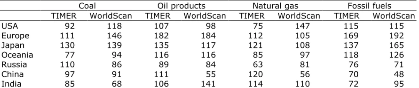
Table 2 compares fossil fuel prices in the BAU in TIMER and WorldScan between various regions. As (tax-inclusive) fuel prices substantially diverge between sectors because of differences in pre-existing taxes, we present average prices for the respective fuels as
observed in the sectors responsible for the largest share of fuel use (i.e. the power sector for coal and natural gas, transport for oil products). Moreover, to compare the overall price level of energy use between regions we also include the average price for the total of fossil fuels consumed (weighted for their volume of consumption).
Both models show relatively high average fuel prices in Europe and Japan, moderate prices in the USA and Oceania and relatively low prices in China, Russia and India. Prices in
WorldScan diverge more between Europe and Japan on the one hand and China on the other hand than prices in TIMER. This might cause more pronounced differences in the results between these regions found by WorldScan than by TIMER. Table 2 also shows more specific differences between the models. In WorldScan, oil prices are relatively low in China and relatively high in India, whereas in TIMER oil prices are somewhat above global average in both countries. For natural gas, TIMER assumes relatively low prices in the USA and relatively high gas prices in Japan and China, whereas in WorldScan the opposite holds. As WorldScan is calibrated on 2004 data and currently assumes a globally uniform development of the price of gas, recent developments in the gas market, in particular the substantial decrease in the price of gas in the USA, are not well included in the model. The differences in relative prices may to some extent contribute differences in results of the models.
Table 2 Tax inclusive fossil fuel prices in 2030 in the BAU relative to global average (= 100) for power sector (coal and natural gas), transport (oil products) and overall weighted average for total fossil fuel consumption
Coal Oil products Natural gas Fossil fuels TIMER WorldScan TIMER WorldScan TIMER WorldScan TIMER WorldScan USA 92 118 107 98 75 147 115 115 Europe 111 146 182 184 112 105 169 192 Japan 130 139 135 117 121 108 137 165 Oceania 77 94 116 116 85 97 118 126 Russia 110 86 89 84 63 81 76 71 China 97 91 111 55 120 56 70 48 India 85 68 106 141 114 110 72 95
Carbon taxes can be introduced over time in different ways. First, the carbon tax can be introduced immediately at the intended level (‘block tax’), keeping it constant afterwards. Second, the tax can be introduced more gradually over time. As WorldScan assumes more or less instantaneous adjustments, results for 2030 will be largely similar for a linearly increasing CO2 tax and a block tax. In TIMER, however, inertia in the energy system (see previous
section) induces different responses to different tax profiles (see also Van Vuuren et al., 2004). To compare the results of TIMER with the instantaneous adjustments in WorldScan, we use a block tax profile for the simulations in TIMER. By introducing the tax immediately in 2010, the energy system in TIMER starts to take into account this emission price in the investments in the energy system from 2010 onwards. By 2030 most of the changes are expected to have been implemented. The simulations by WorldScan assume the introduction of a CO2 tax at a
linearly increasing rate between 2010 and 2020, such that in 2020 the intended level is obtained, which will remain at this level until 2030. This is a pragmatic choice, to avoid WorldScan running into problems to find a numerical solution with high tax levels introduced immediately.
10 Marginal abatement cost curves
Figure 1 presents the MACs up to 100 USD/tCO2 for the year 2030 for 7 world regions: Europe,
USA, Japan, Oceania, Russia, China, and India. These were derived by plotting the incremental levels of a CO2 tax introduced in the models as described above, against the corresponding
reduction in CO2 emissions estimated by the models. The cost curves presented here give a
first impression of the agreement between TIMER and WorldScan on the costs of reducing emissions. In general, reductions tend to be larger in WorldScan than in TIMER for tax levels up to 50 USD/tCO2, which is consistent with findings from other comparison studies (see
Section 2). For higher tax levels, however, reductions in TIMER exceed those in WorldScan for several regions, indicating that further CO2 emission reductions are much more expensive in
WorldScan than in TIMER. In China and Russia, emission reduction rates are higher in WorldScan than in TIMER for the whole range of CO2 tax levels analysed.
The MACs of both TIMER and WorldScan are not strictly convex, i.e. the additional emission reduction associated with an increase in the CO2 tax level by 1 USD/tCO2 is not continuously
decreasing. This can simply be explained by the large potential becoming available at carbon prices around 40 USD/tCO2, especially due to CCS employment (see Figure 1).
Both models show important regional differences. The results of TIMER and WorldScan largely differ for Russia. According to TIMER, Russia is the region with the lowest reduction potential, whereas WorldScan finds relatively high reduction potentials. The most important reason for the low emission reduction potential according to TIMER is the large overcapacity in current coal-fired power plants. This prevents the building of new, low-carbon intensive, power plants. After 2030, most of these power plants are at the end of their lifetime. At that time, replacement of these plants offers opportunities to reduce CO2 emissions. Figure 2 shows that
by 2040 the reduction potential for Russia is much closer to those of the other countries. WorldScan shows the highest reduction potential for China (together with India), whereas according to TIMER, China’s reduction potential is much lower (similar to the average of the other regions). The reason for this lower reduction potential according to TIMER is similar to the reason for Russia: China has expanded its energy sector considerably in the past decade making replacement of or adjustments to these investments very expensive. Hence, moving to low-carbon technologies will be difficult for China. As indicated, WorldScan does not model vintages explicitly and allows for instantaneous adjustments of the energy system. Moreover, WorldScan finds high reduction potential because pre-existing taxes on energy are relatively low implying a relatively energy intensive production structure in the BAU. Hence, China and India have cheaper abatement options than, for instance, Europe, with its relatively high levels of existing taxes on energy. Moreover, with low levels of pre-existing energy taxes, the
introduction of a CO2 tax will have a comparatively large impact on energy.
Finally, TIMER shows a larger reduction potential for India than WorldScan because the energy sector in India will expand significantly in the coming decades. Introducing a carbon tax from 2010 onwards will immediately be taken into account such that the investments will be adjusted to low-carbon technologies at relatively low cost.
11
Figure 1 Marginal abatement cost curves for 2030 resulting from TIMER and WorldScan analyses
Figure 2 Marginal abatement cost curves for 2040 resulting from TIMER analyses
Reduction measures
The outcome of TIMER and WorldScan not only differs in the mitigation rates, but also in the underlying factors through which emission reductions are achieved. A comparison of the reduction measures taken at certain carbon prices provides insight in the differences in the MACs as shown above. Figures 3 to 5 present a decomposition of the emission reductions by 2030 for carbon prices at USD 20, 50 and 100 per tCO2. In the decomposition, the volume
effect refers to a reduction in emissions due to a decrease in the overall size of the economy; the structure effect refers to a reduction in emissions due to a change in the composition of
12
the economy; the efficiency effect refers to a reduction in emissions due to more efficient use of energy; the fossil switch effect refers to a reduction in emissions due to a change in the fossil fuel mix.
At 20 USD/tCO2, differences between TIMER and WorldScan are relatively small for Europe.
For the USA, Japan and Oceania the emission reduction in WorldScan is about 50% higher than in TIMER, mainly because of a larger contribution of efficiency and structure effects. For
Russia, WorldScan finds much larger reduction potential especially due to the implementation of renewable energy and biofuels and the volume and structure effects. These last two effects are not included in TIMER and the use of renewables and biofuels is limited as a result of the overcapacity in power supply. For China and India, WorldScan also finds much larger
reductions at 20 USD/tCO2, especially due to implementation of renewable energy, efficiency
improvements, and volume and structure effects. TIMER simulates a substantial emission reduction in India due to increased use of nuclear energy, whereas in WorldScan we do not model endogenous supply of nuclear energy. As already explained above, the relatively large volume, structure and efficiency effects in Russia, China and India in WorldScan come from the relatively low rates of pre-existing energy taxes.
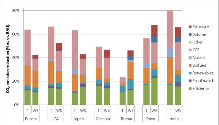
At 50 USD/tCO2, CCS becomes an important mitigation measure in both models. This is not
surprising, since the marginal cost and potential of CCS technology in WorldScan is calibrated according to TIMER results. In Europe, TIMER finds more potential for efficiency
improvements, renewables and CCS and hence a larger overall emission reduction for 50 USD/tCO2. For China, the differences between TIMER and WorldScan are smaller for 50
USD/tCO2 than for 20 USD/tCO2. For India, similar emission reductions are estimated by
TIMER and WorldScan. The contribution of an increased use of bio-energy is larger in TIMER than in WorldScan, whereas volume and structure effects and an increased use of renewables are more important in WorldScan compared to TIMER.
At an even higher carbon price of 100 USD/tCO2, a main difference is that emission
reductions by CCS contribute relatively less to total reduction in WorldScan than in TIMER. As a result, total emission reductions are also smaller in most regions. Although the marginal cost and mitigation potential of CCS in WorldScan is based on the data in TIMER, the actual use of CCS as mitigation option differs, mainly because of differences in the use of coal for electricity generation. Actually, the volume, structure and efficiency effects in WorldScan cause a
13
Figure 3 Decomposition of CO2 emission reduction in 2030 at CO2-tax of $20/ton CO2
– TIMER (T) compared with WorldScan (WS)
Figure 4 Decomposition of CO2 emission reduction in 2030 at CO2-tax of $50/ton CO2
14
Figure 5 Decomposition of CO2 emission reduction in 2030 at CO2-tax of $100/ton
CO2 – TIMER (T) compared with WorldScan (WS)
Mitigation in different coalitions
Both in WorldScan and TIMER, emission reductions in one region depend on climate policies in the rest of the world. The reasons for this dependency are, however, different between the models. In WorldScan, the reason is that the net effect on CO2 emissions as calculated for a
specific region not only reflects the primary impact of the CO2 tax through adjustments of
domestic production and consumption patterns, but also secondary effects due to changes in exports and imports and hence in international prices. In TIMER, learning-by-doing plays an important role: with smaller coalitions there is less learning-by-doing on a global scale, which negatively impacts future potential at a given carbon price. On the other hand, in a smaller coalition there is less global demand for bioenergy, which means lower feedstock prices for bioenergy (either for fuel or power).
To provide some insight into the above effects, we analysed CO2 mitigation in Europe for
international climate coalitions different from a CO2 tax introduced in all regions in the world
(Uniform, as presented above). In particular, we consider a policy case in which Europe and all other Annex 1 countries introduce a CO2 tax (Annex1), and a case in which Europe is the only
region in the world introducing a CO2 tax (Unilateral).
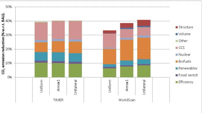
Figure 6 shows the results of WorldScan for these different cases for CO2 emission reduction
in Europe next to the results of TIMER for the Uniform case. The results show that in both WorldScan and TIMER, the Annex1 and Unilateral scenarios lead to higher emission reductions in Europe at a carbon tax of 50 USD/tCO2. In WorldScan, the main reason is that
energy-intensive activities are outsourced, as reflected by the increasing contribution of the structure and volume effects in total mitigation. A worldwide introduction of a CO2 tax (Uniform) makes
production by the energy intensive sectors in Europe more competitive and production
volumes in these sectors increase compared with the BAU. If other regions, such as China, will not introduce a similar CO2 tax, European industry will face a loss of competitiveness and
15
climate policies. Note that this outsourcing limits the effectiveness of climate policies in terms of reducing worldwide CO2 emissions, as this causes carbon leakage to other regions (see
Bollen et al., 2012). Moreover, emission reductions by efficiency improvements and the use of biofuels increases, which can be explained by the reduction in global fossil fuel prices due to climate policies, which is smaller with less countries joining the international climate coalition. In TIMER, the Annex1 and Unilateral scenarios lead to (slightly) higher reductions due to the use of biofuels induced by lower feedstock prices for bioenergy. This effect is larger than the learning-by-doing effect, which results in less emission reductions by efficiency improvements.
Figure 6 Decomposition of CO2 emission reduction in Europe in 2030 at a CO2 tax
level of 50 USD/tCO2 for different international climate coalitions (Uniform: CO2 tax
in all regions; Annex1: CO2 tax in Annex 1 regions; Unilateral: CO2 tax in Europe only)
5
Comparison of cost estimates
Different indicators can be used to analyse how policies affect social welfare. One (partial) indicator is the welfare costs of policies, i.e. the value of the resources society is willing to give up to take a given course of action, such as a predetermined reduction in CO2 emissions (see
e.g. Krupnick and McLaughlin, 2011). To evaluate overall welfare effects of emission
reductions, also the benefits of this reduction should be included. Both FAIR and WorldScan provide estimations of the welfare cost of policies. In order to allow for analyses of both the benefits and the cost of climate policies, FAIR provides estimates of the benefits of reduced global warming (Hof et al., 2008) and the direct cost of mitigation measures. FAIR also calculates consumption losses due to climate policies, based on a simple Cobb-Douglas production function (see Appendix). WorldScan only includes welfare cost of climate policies, measured by the Hicksian Equivalent Variation. This measure is usually presented as a
percentage of national income in the BAU showing the loss of welfare in terms of a reduction in national income.4 As WorldScan does not provide a measure for the benefits of emission
reduction, the model clearly provides a partial measure of the social welfare effects of policies.
4 The Hicksian Equivalent Variation of a policy case measures the amount of money by which the income of households in the
16
The focus here is only on the various measures for welfare cost provided by FAIR and WorldScan. The outcome of WorldScan calculations includes various indicators to measure the economic impact of climate policies, including the change in GDP (as a measure for overall economic activity), consumption and national income. TIMER/FAIR present direct cost of
mitigation measures as a percentage of GDP in the BAU and associated consumption losses. As these various indicators are not directly comparable, the main focus of the comparison here is on the distribution of the cost over regions according to the various measures.
As indicated, economic welfare effects are different from direct cost estimates. Indirect effects cause a redistribution of costs over economic actors and regions and may exceed the direct cost because of market failures. To analyse the relevance of this difference, in this section we compare the direct costs and consumption losses in various regions as estimated by TIMER/FAIR and the change in GDP, consumption and economic welfare of a comparable climate policy scenario as calculated by WorldScan. Note that in TIMER/FAIR the direct costs in a certain year do not take into account abatement action in previous years, in contrast to consumption losses.
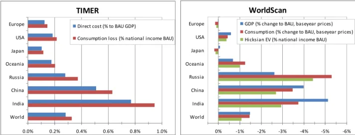
Figure 7 compares the cost estimated by FAIR and WorldScan for a globally uniform CO2 tax
of 50 USD/tCO2. Obviously, all regions face direct cost as a result of the introduction of a CO2
tax. Both in FAIR and in WorldScan a CO2 tax stimulates investments in mitigation which
involves additional cost for producers and consumers. Graphically this is the area below the MACs in Figure 1 up to the level of 50 USD/tCO2. In proportion to the level of GDP, direct costs
are particularly high in regions with relatively high levels of CO2 emissions in proportion to
GDP, such as India and China. The economic impacts as calculated by WorldScan are
somewhat different as they take into account a redistribution of the costs over regions as well as additional indirect effects (see Section 2). In terms of GDP losses, WorldScan results also show large effects in particular in India and China (5% and 4% below BAU respectively). An interesting finding of WorldScan is that GDP in Europe and Japan is hardly affected by the CO2
tax, in contrast to FAIR. This can be explained by the fact that Europe and Japan are less energy- and CO2-intensive than most other regions. As a result, the CO2 tax will have less
impact on production cost than in other regions, which makes producers EU and Japan more competitive. This results in more export of energy-intensive products, mitigating the negative pressure of the carbon tax.
Consumption losses as calculated by FAIR show a similar pattern of distribution over regions as the direct cost in relation to GDP. The change in consumption as calculated by WorldScan shows a somewhat different behaviour than change in GDP. In Russia the change in
consumption is more than double the change in GDP. This follows from the fact that Russia, as a large oil and gas exporter, experiences a deterioration in its terms-of-trade because of
decreasing fuel prices. To a lesser degree this also applies to Oceania as a major coal exporter. On the other side, Europe and Japan manage to increase their consumption, notwithstanding the CO2 tax. This can be attributed to improvements in their terms-of-trade and
competitiveness. Consumption losses as calculated by FAIR turn out to be much smaller than those found by WorldScan. Possible explanations for these differences are: (i) in FAIR,
mitigation costs are only for a small part (~20%) deducted from investments, leading to relatively small indirect cumulative effects; and (ii) FAIR does not account for climate policy making consumption more expensive, which implies a lower reduction of consumption volume compared to WorldScan.
As welfare losses are related to consumption (see Appendix), the Hicksian Equivalent Variation as determined by WorldScan shows a similar pattern as the change in consumption: welfare losses are largest in Russia, India and China, and Europe and Japan are even better off in terms of economic welfare.
17
Figure 7 Comparison of cost measures in 2030 by TIMER and WorldScan for global uniform CO2 tax of 50 USD/tCO2. TIMER: direct costs as % of BAU GDP and
consumption loss as % of BAU; WorldScan: welfare effects as Hicksian Equivalent Variation as % of BAU national income, GDP and national income as % change to BAU.
Comparison with other studies on cost of climate policies
Van Vuuren et al. (2009) found that for regimes that assume participation of developed and developing countries long-term direct abatement costs correlate strongly with macroeconomic costs for most regions. This was also shown for oil-exporting regions as in general these regions have highly carbon intensive economies leading also to high abatement costs. Still, Van Vuuren et al. (2009) acknowledge that there are economic impacts that are not included in the direct abatement costs such as the impact of income losses via changes in fuel trade.
Studies using CGE models to analyse the global impact of climate policies confirm that partial analyses based on direct cost of mitigation only, may lead to other conclusions than analyses of welfare effects in various regions using a general equilibrium framework. Böhringer et al. (2010) show climate policies in the USA and Europe only to cause large welfare losses in oil exporting regions. Other regions, including Japan and India, benefit from lower international fossil fuel prices. Morris et al. (2008) show that there is little correspondence between the marginal abatement cost and the marginal welfare cost. Moreover they show that the welfare effects in a region may largely diverge for different mitigation rates in the region and in the rest of the world. The analyses by Peterson et al. (2011), Dellink et al. (2011) and McKibbin et al. (2011) show comparable mechanisms as occur in WorldScan. As the policy cases simulated in these studies are not the same as the policy cases in this paper it is not possible to directly compare the results. This requires further analysis of welfare effects estimated by WorldScan, which was however beyond the scope of this study.
6
Conclusions and future work
Based on differences and explanation of differences between results of TIMER and WorldScan, we summarize the following:
• for CO2 tax rates up to 50 USD/tCO2 differences between estimated emission reductions
are limited for developed regions, but large in some developing regions;
• the mitigation potential in WorldScan hardly changes over time, whereas TIMER shows changes resulting from the dynamics in the energy system as well as the effects of technological change due to learning by doing;
WorldScan
-6% -5% -4% -3% -2% -1% 0% Europe USA Japan Oceania Russia China India WorldGDP (% change to BAU, baseyear prices) Consumption (% change to BAU, baseyear prices) Hicksian EV (% national income BAU)
TIMER
0.0% 0.2% 0.4% 0.6% 0.8% 1.0% Europe USA Japan Oceania Russia China India WorldDirect cost (% to BAU GDP)
18
• inertia in the energy system as included in TIMER result in emission reductions
estimated by TIMER to be substantially smaller than those estimated by WorldScan for Russia and China. In this regard, WorldScan seems to be too optimistic about mitigation potential of renewables and biofuels, particularly in regions which have substantially expanded their energy production sector recently;
• in case of a global uniform CO2 tax, emission reductions through changes in the overall
level of production and consumption in a region (volume effect) and through changes in the structure of the economy (structure effect) tend to be less important in developed economies. In regions with no or low rates of pre-existing energy taxes WorldScan estimates substantial emission reductions through volume and structure effects, which significantly contributes to mitigation rates being higher in WorldScan than in TIMER; • for higher CO2 tax rates, the use of biofuels as estimated by WorldScan is substantially
smaller than estimated by TIMER;
• the mitigation rates in a specific region depend on the international context of climate policies. For a given carbon tax level, WorldScan and TIMER project higher emission reductions in Europe with smaller coalitions, but for different reasons. The reason in WorldScan is the impact of changes in international trade and other indirect effects, while feedstock prices for bioenergy and learning-by-doing are the main reason in TIMER.;
• the distribution of the direct cost of climate policies over regions is different from the distribution of the economic welfare losses as a result of indirect effects.
Strengths and weaknesses of TIMER and WorldScan
Based on these findings, we conclude that TIMER and WorldScan have their strengths and weaknesses on different aspects, which are all relevant for the assessment of climate policies. Given the detailed modelling of the energy system in TIMER, the strengths of TIMER are in the analysis of:
- consequences of climate policies for the entire energy system;
- technology specific development, including learning by doing and physical constraints; - development of the responses to climate policies over time;
- long-term climate policies (>20 years);
- consequences of climate policies to specific economic actors;
- within the IMAGE integrated assessment framework, a combination of TIMER and FAIR allows to assess the mitigation potential and costs of GHG emissions both from the energy and land-use systems.
By taking into account indirect effects of climate policies and consequences for international trade, the strengths of WorldScan are in the analysis of:
- changes in demand for goods and services as a result of climate policies;
- redistribution of the economic welfare losses due to climate policies over sectors and regions;
- macro-economic consequences (structure of the economy, volume of production and consumption) of climate policies;
- global effectiveness of climate policies that do not encompass the whole world, by taking into account potential carbon leakage;
19
Table 3 Overview of strengths and weaknesses of TIMER/FAIR and WorldScan
TIMER/FAIR WorldScan energy system consequences of climate policies
for the entire energy system at detailed, i.e. technology specific level
consequences of climate policies for entire economy, including energy system at high level of aggregation
feasibility of mitigation options in
energy system Accounting for physical constraints and data on installed capacity in the energy system
applicability of mitigation options exogenous to the model; no information on installed capacity, instantaneous adjustment at no cost
development of response to
climate policies over time dynamics in the energy system and technological change through learning by doing, dependent on installed capacity
exogenous change in cost and potential of wind, biomass and CCS, derived from TIMER time horizon well able to analyse long-term
consequences of climate policies (> 20 years) by taking into account technological change and (physical) constraints to the energy system
best fit to analyse consequences of climate policies for global economy reaching a new equilibrium situation with time horizon of ~20 years; not able to analyse drastic changes in energy system so not very well suitable for long-term analysis of far-reaching climate policies structural changes behavioural changes due to
changes in relative prices not included
both technical measures and structural changes are considered as mitigation options; in regions with no or low rates of pre-existing energy taxes behavioural changes significantly contribute to mitigation
international climate policies effect of climate policies in other regions on mitigation rates in one region are negligible
mitigation in one region
dependent on (climate) policies in other regions through indirect effects
distribution of costs and welfare
effects TIMER/FAIR only takes into account the direct cost, i.e. the cost of mitigation that actors initially incur
by taking into account the indirect effects, WorldScan estimates a redistribution of the cost (e.g. through terms of trade effects); moreover, market distortions, such as pre-existing taxes on energy, cause welfare effects to be significantly different from the direct cost
carbon leakage effect of climate policies in one region on economic activities in the rest of the world are negligible
climate policies in one region will affect international trade and prices and hence economic activities and related emissions
In conclusion we can say that in cost assessments of climate policies, results by WorldScan complement the analyses made by TIMER, in particular with respect to the regional distribution of those costs. This effect will be even greater in analyses on climate coalitions that do not include all countries in the world. Moreover, analyses by WorldScan require a complementary assessment by TIMER on the technological aspects of the changes in the energy system. Exploiting the complementary insights of both models will provide a set of models that is very well suitable to assess the various impacts of climate change policies.
20 Future work
In addition to differences between the models that are the result of their different scope and structure, there are differences related to specific assumptions in the models that can, to some extent, be removed. Therefore, we propose a limited number of future actions to further align the models. These concern:
• tuning the data on cost and potential of biofuels use as included in WorldScan to the information in TIMER (or actually IMAGE) which not only takes into account issues with respect to the energy system, but also related to land use; given the observed
differences in biofuel use at different CO2 tax rates between TIMER and WorldScan this
is expected to bring the WorldScan results closer to TIMER. This might also require changes to the way land-use activities are modelled in WorldScan;
• WorldScan currently assumes a globally uniform development of the price of natural gas. As this does not match recent developments of substantially decreasing gas prices in the USA compared with prices in Europe and Asia, WorldScan will be adapted to reflect regional differences in the development of fossil fuel prices;
• a further investigation of the impact differences in energy prices between TIMER and WorldScan may have on the effect of a CO2 tax;
• in TIMER the lifetime of energy investments is exogenous; this causes the inertia in the energy system to be somewhat overrated, as high carbon taxes certainly will reduce the economic lifetime of carbon-intensive production facilities, such as inefficient coal-fired power plants. Considering this may result in larger reductions in emissions, in particular in Russia, and hence bring the TIMER results closer to WorldScan;
• the long-term effects of abatement costs on consumption losses are rather small in FAIR, due to default parameter settings in the economic growth module. Sensitivity analyses on these parameter settings could provide more insight into the uncertainty in long-term effects on consumption losses. Moreover, the economic growth module could be extended by, for instance, including the effects of fuel trade on consumption losses; • it might also be useful to consider the adoption of vintages in WorldScan to take into
21
References
Amann M., Rafaj P., Höhne N., 2009. GHG mitigation potentials in Annex I countries. Comparison of model estimates for 2020. IIASA Interim Report. International Institute for Applied Systems Analysis (IIASA).
Babiker M., Gurgel A., Paltsev S., Reilly J., 2009. Forward-looking versus recursive-dynamic modeling in climate policy analysis: A comparison. Economic Modelling 26, 1341-1354.
Boeters S., Koornneef J., 2011. Supply of renewable energy sources and the cost of EU climate policy. Energy Economics 33, 1024-1034.
Böhringer C., Fischer C., Rosendahl K.E., 2010. The global effects of subglobal climate policies. The B.E. Journal of Economic Analysis & Policy 10, Article 13.
Böhringer C., Rutherford T.F., 2008. Combining bottom-up and top-down. Energy Economics 30, 574-596.
Bollen J., Brink C., 2012. Air pollution policy in Europe: quantifying the interaction with greenhouse gases and climate change policies. PBL Working Paper. CPB Netherlands Bureau for Economic Policy Analysis/PBL Netherlands Environmental Assessment Agency, The Hague. Bollen J., Brink C., Koutstaal P., Veenendaal P., Vollebergh H., 2012. Trade and Climate Change: Leaking Pledges. CESifo DICE Report 10, 44-51.
Bosetti V., Carraro C., Duval R., Tavoni M., 2011. What should we expect from innovation? A model-based assessment of the environmental and mitigation cost implications of climate-related R&D. Energy Economics 33, 1313-1320.
Bouwman A.F., Kram T., Klein Goldewijk K. (Eds), 2006. Integrated modelling of global environmental change. An overview of IMAGE 2.4. Netherlands Environmental Assessment Agency (MNP), Bilthoven, The Netherlands.
Clapp C., Karousakis K., Buchner B., Chateau J., 2009. National and sectoral GHG mitigation potential: a comparison across models. COM/ENV/EPOC/IEA/SLT(2009)7. OECD/IEA, Paris. Dellink R., Briner G., Clapp C., 2011. The Copenhagen Accord/Cancún Agreements emission pledges for 2020: exploring economic and environmental impacts. Climate Change Economics 2, 53-78.
Den Elzen M.G.J., Mendoza Beltran A., Hof A.F., Van Ruijven B., Van Vliet J., 2013. Reduction targets and abatement costs of developing countries resulting from global and developed countries’ reduction targets by 2050. Mitig Adapt Strateg Glob Change 18, 491-512. Fankhauser S., Tol R.S.J., 2005. On climate change and economic growth. Resource and Energy Economics 27, 1-17.
Hayden M., Veenendaal P.J.J., Žarnić Ž., 2010. Options for international financing of climate change mitigation in developing countries. Economic Papers 406. European Commission, Directorate-General for Economic and Financial Affairs, Brussels.
Hof A.F., Den Elzen M.G.J., Van Vuuren D.P., 2008. Analysing the costs and benefits of climate policy: Value judgements and scientific uncertainties. Global Environmental Change 18, 412-424.
Klepper G., Peterson S., 2006. Marginal abatement cost curves in general equilibrium: The influence of world energy prices. Resource and Energy Economics 28, 1-23.
22
Krupnick A.J., McLaughlin D., 2011. GDP, consumption, jobs, and costs: Tracking the effects of energy policy. Issue Brief 11-08. Resources for the Future (RFF), Washington DC.
Lejour A., Veenendaal P.J.J., Verweij G., van Leeuwen N., 2006. WorldScan: a Model for International Economic Policy Analysis. CPB Document 111. CPB Netherlands Bureau for Economic Policy Analysis, Den Haag.
Manders T., Veenendaal P., 2008. Border tax adjustments and the EU-ETS. A quantitative assessment. CPB Document 171. CPB Netherlands Bureau for Economic Policy Analysis, PBL Netherlands Environmental Assessment Agency, Den Haag, The Netherlands.
Markandya A., Halsnaes K., Lanza A., Matsuoka Y., Maya S., Pan J., Shogren J.F., Seroa de Motta R., Zhang T., 2001. Costing methodologies. In: Metz B, Davidson O, Swart RJ, Pan J (Eds), Climate change 2001. Mitigation. IPCC, Working Group III. Cambridge University Press, Cambridge, UK; 2001. pp. 451-498.
McKibbin W., Morris A.C., Wilcoxen P.J., 2011. Comparing climate commitments: a model-based analysis of the Copenhagen Accord. Climate Change Economics 2, 79-103.
Messner S., Schrattenholzer L., 2000. MESSAGE–MACRO: linking an energy supply model with a macroeconomic module and solving it iteratively. Energy 25, 267-282.
Miketa A., 2004. Technical description on the growth study datasets. Environmentally Compatible Energy Strategies Program, International Institute for Applied Systems Analysis (IIASA), Laxenburg, Austria.
Morris J., Paltsev S., Reilly J.M., 2008. Marginal abatement costs and marginal welfare costs for greenhouse gas emissions reductions: results from the EPPA model. Report. MIT Joint Program on the Science and Policy of Global Change, Cambridge, USA.
Narayanan B., Walmsley T.L. (Eds), 2008. Global Trade, Assistance, and Production: The GTAP 7 Data Base. Center for Global Trade Analysis, Purdue University,
Nordhaus W.D. A question of balance: weighing the options on global warming policies. Yale University Press; 2008.
OECD, 2012. OECD Environmental Outlook to 2050: The consequences of inaction. OECD, Paris.
Paltsev S., Reilly J.M., Jacoby H.D., Tay K.H., 2007. How (and why) do climate policy costs differ among countries? In: Schlesinger M, Kheshgi H, Smith J, de la Chesnay F, Reilly JM, Wilson T, Kolstad CD (Eds), Human-Induced Climate Change: An Interdisciplinary Assessment. Cambridge University Press, Cambridge, UK; 2007. pp. pp. 282-293.
Peterson E.B., Schleich J., Duscha V., 2011. Environmental and economic effects of the Copenhagen pledges and more ambitious emission reduction targets. Energy Policy 39, 3697-3708.
Piermartini R., Teh R., 2005. Demystifying modelling methods for trade policy. WTO Discussion Papers No. 10. World Trade Organization, Geneva.
Richels R.G., Blanford G.J., 2008. The value of technological advance in decarbonizing the U.S. economy. Energy Economics 30, 2930-2946.
Richmond A., Kaufmann R.K., Myneni R.B., 2007. Valuing ecosystem services: A shadow price for net primary production. Ecological Economics 64, 454-462.
23
Van Vuuren D., Den Elzen M., Lucas P., Eickhout B., Strengers B., Van Ruijven B., Wonink S., Van Houdt R., 2007. Stabilizing greenhouse gas concentrations at low levels: an assessment of reduction strategies and costs. Climatic Change 81, 119-159.
Van Vuuren D.P., 2006. Energy systems and climate policy - Long-term scenarios for an uncertain future. PhD Thesis, Dept. of Science, Technology and Society, Faculty of Science, Utrecht University.
Van Vuuren D.P., De Vries B., Eickhout B., Kram T., 2004. Responses to technology and taxes in a simulated world. Energy Economics 26, 579-601.
Van Vuuren D.P., Hoogwijk M., Barker T., Riahi K., Boeters S., Chateau J., Scrieciu S., Van Vliet J., Masui T., Blok K., Blomen E., Kram T., 2009. Comparison of top-down and bottom-up estimates of sectoral and regional greenhouse gas emission reduction potentials. Energy Policy 37, 5125-5139.
Vollebergh H.R.J., Kemfert C., 2005. The role of technological change for a sustainable development. Ecological Economics 54, 133-147.
24
Appendix – description of the models used
TIMER and FAIR
TIMER is an energy-system simulation model, describing the demand and supply of 12 different energy carriers for a set of world regions. Its main objective is to analyse the long-term trends in energy demand and efficiency and the possible transition towards renewable energy sources. Within the context of IMAGE, the model describes energy-related GHG and air pollution emissions, along with land-use demand for energy crops. The TIMER model focuses particularly on several dynamic relationships within the energy system, such as inertia, learning-by-doing, depletion and trade among the different regions. The TIMER model is a simulation model, which means that the results depend on a single set of deterministic algorithms instead of being the result of an optimization procedure.
Model structure
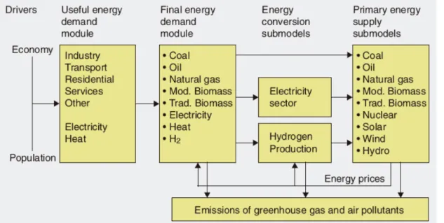
The TIMER model describes the chain from demand for energy services (useful energy) to the supply of energy by different primary energy sources and related emissions (Figure A.1). The steps are connected by demand for energy (from left to right) and by feedbacks, mainly in the form of energy prices (from right to left). The TIMER model has three types of submodels: (i) the energy demand model; (ii) models for energy conversion (electricity and hydrogen
production), and (iii) models for primary energy supply. Some of the main assumptions for the different sources and technologies are listed in Table A.1
Figure A.1 Schematic representation of the TIMER model
Energy demand submodel
Final energy demand (for five sectors and eight energy carriers) is modelled as a function of changes in population, in economic activity and in energy intensity (Figure A.1). The model distinguishes four dynamic factors: structural change, autonomous energy efficiency
improvement, price-induced energy efficiency improvement and price-based fuel substitution, which are discussed below.
25