Cumulative exposure to residues of plant protection products via food in the Netherlands | RIVM

(1)

(2)

(3)

Netherlands

RIVM Letter report 2018-0018 P.E. Boon et al.

(4)

Colophon

Parts of this publication may be reproduced, provided acknowledgement is given to: National Institute for Public Health and the Environment, along with the title and year of publication.

DOI 10.21945/RIVM-2018-0018

P.E. Boon (author), RIVM

G. van Donkersgoed (author), RIVM J.D. te Biesebeek (author), RIVM G. Wolterink (author), RIVM A.G. Rietveld (author), RIVM Contact:

Anton Rietveld

Department of Food Safety anton.rietveld@rivm.nl

This study was commissioned by the Ministry of Health, Welfare and Sports within the framework of project V/050317

This is a publication of:

National Institute for Public Health and the Environment

P.O. Box 1 | 3720 BA Bilthoven The Netherlands

(5)

Synopsis

Cumulative exposure to residues of plant protection products via food in the Netherlands

People are exposed to residues of different plant protection products via food. This can be due to the consumption of different foods which contain different residues or because more than one residue is present in a food product. RIVM has analysed this so called cumulative exposure to residues from plant protection products via food.

In this study, substances that may affect the thyroid and those that may affect the nervous system were included. The current exposure to these substances is not likely to cause a health effect on the thyroid. With regard to the substances that may affect the nervous system a risk cannot be excluded. This is because the margin between the calculated exposure and the limit that is considered safe is relatively small. The real exposure is most likely lower than the calculated exposure, due to uncertainties in the calculation.

Cumulative exposure assessment is based on the assumption that only substances that affect the same organ should be summed.

To analyse the safety of cumulative exposure to all residues of plant protection products via food, it is necessary to determine which substances should be summed for other organs than the thyroid and nervous system. The European Food Safety Authority (EFSA) is currently working on further grouping of substances. This requires analysis of all the available data on adverse effects of residues in plant protection products.

Keywords: cumulative exposure, young children, children, adults, older adults, plant protection products, probabilistic

(6)

(7)

Publiekssamenvatting

Gelijktijdige blootstelling aan residuen van

gewasbeschermingsmiddelen via voedsel in Nederland

Mensen worden via voedsel blootgesteld aan stoffen uit

gewasbeschermingsmiddelen. Dit kan door verschillende soorten voedsel te eten waar verschillende stoffen op zitten, en doordat meerdere

stoffen op één soort voedsel kunnen zitten. Het RIVM heeft een inschatting gemaakt van deze gelijktijdige blootstelling aan stoffen uit gewasbeschermingsmiddelen, zogenoemde cumulatieve blootstelling, via voedsel.

In deze studie gaat het om stoffen die effecten op de schildklier en het zenuwstelsel kunnen hebben. De huidige gelijktijdige blootstelling aan deze stoffen heeft geen schadelijke effecten op de schildklier. Voor de stoffen die effect kunnen hebben op het zenuwstelsel kan het RIVM een risico niet uitsluiten. Dat is omdat de marge tussen de hoeveelheid die we binnenkrijgen en de hoeveelheid die als veilig wordt gezien dicht bij elkaar liggen. De werkelijke blootstelling is zeer waarschijnlijk lager dan de berekende blootstelling. Dat komt door onzekerheden in de

berekeningen.

Het uitgangspunt van het onderzoek is dat de hoeveelheden van stoffen die op eenzelfde orgaan hun uitwerking hebben, bij elkaar worden opgeteld.

Het is nog niet mogelijk om een uitspraak te doen over de veiligheid van de gelijktijdige blootstelling aan alle stoffen uit

gewasbeschermingsmiddelen via voedsel. Hiervoor moet eerst worden bepaald welke stoffen effecten op andere organen dan de schildklier en het zenuwstelsel kunnen hebben. De Europese

voedselveiligheidsautoriteit EFSA werkt momenteel aan deze indeling. Hiervoor is een analyse nodig van de beschikbare gegevens over de schadelijke effecten van alle stoffen in gewasbeschermingsmiddelen. Kernwoorden: gelijktijdige blootstelling, jonge kinderen, kinderen, volwassenen, ouderen, bestrijdingsmiddelen, probabilistisch

(8)

(9)

Appendix S. Contribution of raw agricultural commodities (‘foods as measured’), substances (‘compounds’) and substance/raw agricultural commodity combinations to the upper 0.1% of the acute cumulative exposure distribution of CAG-neurochemical for the four age groups — 80

Appendix T. Contribution of raw agricultural commodities (‘foods as measured’), substances (‘compounds’) and substance/raw agricultural commodity combinations to the upper 0.1% of the chronic cumulative exposure distribution of CAG-motor division for the four age groups — 82

(12)

(13)

1 Introduction

People are exposed to different residues of plant protection products (PPPs) (or pesticides) via food, either via the consumption of different foods which contain one or more residues of PPPs and/or because more than one residue is present in single food product. This has raised the question whether simultaneous exposure to multiple residues of PPPs via food, so-called cumulative exposure, is safe for consumers.

Over the past years, the European Commission (EC) and its Member States, the European Food Safety Authority (EFSA) and independent scientists have worked on a methodology to estimate cumulative

exposure via food (EFSA, 2008; 2009; 2012; van Klaveren et al., 2010). In 2010-2013, the RIVM coordinated the EU project ACROPOLIS;

Aggregate and Cumulative Risk Of Pesticides: an On-Line Integrated Strategy1_{. A web-based model was developed to assess cumulative} exposure via food (van der Voet et al., 2015) and cumulative exposure assessments were performed for eight European countries (Boon et al., 2015). In addition, EFSA’s Panel on Plant Protection Product and their Residues (PPR Panel) has put effort into defining groups of active substances in PPPs that may cause the same toxic effects in tissues, organs and physiological systems – even if they do not share the same mode of action (EFSA, 2013). These groups of substances are called cumulative assessment groups (CAGs). To assess potential risks related to the exposure to such groups of substances via food, a cumulative dietary exposure assessment should be performed. In such an assessment, the exposure to all substances within a CAG via food is estimated. In 2013, the PPR Panel established several CAGs regarding acute and chronic effects on the nervous system and regarding chronic effects on the thyroid (EFSA, 2013).

In 2015, EFSA and RIVM established a Framework Partnership Agreement (FPA). As part of this agreement, RIVM estimated the

cumulative dietary exposure to two of the CAGs for acute effects on the nervous system (a CAG for neurochemical effects, i.e. inhibition of acetylcholinesterase activity, and a CAG for effects on the motor division) and two CAGs for chronic effects on the thyroid (one CAG for effects on the parafollicular (C-) cells or the calcitonin system and one CAG for effects on follicular cells and/or thyroid hormone

(triiodothyronine-T3 and thyroxine-T4 system). In 2016, EFSA provided an update on the composition of these four CAGs for use in that study, as well as information on the potency of the substances to produce the common effect. To estimate the cumulative exposure to these CAGs, food consumption data from different dietary surveys conducted in European countries and concentration data from European monitoring programmes were used. Data from the Netherlands were included in this study. As this assessment was commissioned by EFSA within the FPA, the results will be published on the EFSA website. Publication is foreseen

(14)

in the second half of 2018. For the other CAGs defined in 2013, no update was provided by EFSA.

In November 2017, a Dutch newspaper2_{published an item about}

multiple residues on strawberry, entitled ‘Strawberries six times more toxic than other fruit due to cocktail effect’. Questions were raised in the Dutch House of Representatives regarding the methods available for performing a cumulative risk assessment. In response, the Dutch

Ministry of Health, Welfare and Sports (VWS) has commissioned RIVM to calculate the cumulative dietary exposure of the Dutch population to the two CAGs regarding acute effects on the nervous system and the two CAGs regarding chronic effects on the thyroid. To this end, RIVM has used the most recent Dutch food consumption data and residue data of PPPs from Dutch monitoring programmes. In this report, the results of this assessment are described.

(15)

2 Exposure calculations

To calculate the exposure to substances present in food, information about the amount and types of foods consumed within the population of interest is needed, as well as information on the concentrations of these substances in the foods consumed. If substances are measured in unprocessed foods, effects of food handling (e.g. peeling and cooking) on the concentration of the substances in the foods as consumed should preferably also be included, if available. Finally, a computational tool is needed to combine these data in such a way that a meaningful

estimation of the exposure is obtained.

In this section, the input data and methodology used for assessing the cumulative exposure are described. The methodology used is consistent with the most refined exposure scenario (‘tier 2 scenario b’) used in the 2017 cumulative study, referred to as the ‘FPA study’ in the rest of this report.

2.1 Cumulative assessment groups

Cumulative exposure is only meaningful for substances that may cause the same toxic effects in tissues, organs and physiological systems (EFSA, 2013). In this report, the cumulative exposure via food to four of such cumulative assessment groups (CAGs) was calculated; two were defined as having a potential acute effect on the nervous system and two as having a potential chronic effect on the thyroid:

• The CAG covering acute neurochemical effects, i.e. inhibition of acetylcholinesterase activity (CAG-neurochemical);

• The CAG covering acute functional effects on motor division (CAG-motor division);

• The CAG covering chronic effects on parafollicular (C-)cells or the calcitonin system (CAG-calcitonin)

• The CAG covering chronic effects on follicular cells and/or the thyroid hormone (T3/T4) system (CAG-thyroid hormone).

The substances per CAG were provided by EFSA as part of the FPA study and are listed in Appendices A, B, C and D.

2.2 The relative potency factor (RPF) approach

When estimating the exposure to a group of substances, differences in the potency to produce the same toxic effect between the substances within the same group should be considered. For this, the relative potency factor (RPF) approach can be used. In this approach, the potency of the active substances (hereafter referred to as just ‘substances’) belonging to a CAG is expressed relative to that of one selected substance within the CAG, a so-called “index compound”. The potency of a substance reflects its ability to cause harm and is

expressed either as a no-observed adverse effect level (NOAEL) or lower limit of a benchmark dose (BMDL), both in mg/kg body weight (bw). The NOAEL reflects the dose at which no adverse effect is observed in an animal toxicity study. The BMDL reflects the dose at which a predefined change (e.g. 5% increase) in an effect occurs in an animal or

(16)

epidemiological study. The relative potency of a substance is expressed as a factor of the potency of the index compound. For example, the RPF of a substance is two, when the NOAEL or BMDL of the index compound is twice the NOAEL or BMDL of the substance. See Box 1 for an example of the calculation of an RPF for a substance.

Box 1: Calculation relative potency factor (RPF) for carbofuran

Carbofuran, belonging to the CAG-neurochemical, has a NOAEL of 0.015 mg/kg bw and the index compound oxamyl has a NOAEL of 0.1 mg/kg bw. This results in a RPF of 6.67 for carbofuran. In the

calculations, carbofuran is thus considered to be 6.67 times more potent than the index compound oxamyl.

The RPFs per substance are subsequently used to convert single

substance concentrations to one cumulative concentration per analysed sample. This adjusted concentration is then used as input for the cumulative exposure assessment. See Box 2 for an example of such a calculation.

Box 2: Calculation cumulative concentration of an analysed sample

A CAG consists of three substances (A, B and C). One food sample has been analysed for all three substances at following concentrations: A: 0.05 mg/kg; B: 0.10 mg/kg; C: 0.07 mg/kg

The relative potency factors of these compounds are A: 1; B: 2; C: 0.25.

Substance A is the “index compound”.

The cumulative concentration expressed in equivalents of the index compound of this food sample can then be calculated as

(0.05 × 1) + (0.10 × 2) + (0.07 × 0.25)

= 0.27 mg/kg A equivalents. In the present study, the RPF approach was used to calculate the

cumulative exposure to the four CAGs. The RPFs were provided by EFSA within the FPA study. These RPFs were based on NOAELs, using oxamyl as index compound for the CAGs regarding acute effects on the nervous system. For the CAGs regarding chronic effects on the thyroid,

fenbuconazole was used as the index compound for the CAG-calcitonin and ioxynil for the CAG-thyroid hormone. The NOAELs and RPFs per substance and per CAG are listed in Appendices A, B, C and D.

2.3 Food consumption data

To assess the exposure to substances belonging to the four CAGs, food consumption data from the Dutch National Food Consumption Survey (DNFCS) were used. Data were available for three age groups: 2 to 6 years, 7 to 69 years and 70+ years. In the FPA study, only the

consumption data of the youngest children (2 to 6 years) were included. The food consumption data for children aged 2 to 6 were obtained from the DNFCS-Young children conducted in 2005 and 2006 (Ocké et al., 2008). The data for the population aged 7 to 69 were obtained from the DNFCS 2007-2010 (van Rossum et al., 2011), and those for the

(17)

population aged 70 + from DNFCS 2010-2012 (Ocké et al., 2013). For a detailed description of the three surveys, see Appendix E.

The food consumption were coded according to the FoodEx1

classification system (EFSA, 2011). FoodEx1 is a hierarchical system based on 20 main food categories that are further divided into

subgroups up to a maximum of four levels. Level 4 is the most refined (e.g. bread) and level 1 is the least refined (e.g. grains and grain-based products). The food consumption data were coded at the most refined level as possible, most at level 4. This coding system was used to be in line with the FPA study.

2.4 Residue data

Thirty raw agricultural commodities (RACs), covering widely consumed commodities in the Netherlands were selected for the exposure

assessment. These commodities included the 28 commodities to be sampled in 2016, 2017 and 2018 within the EU-coordinated programme (EUCP)3_{(apple, aubergine, banana, beans (with pods), broccoli, carrot,} cauliflower, cucumbers, head cabbage, leek, lettuce, mandarin, olives for oil production, orange, peach, pear, peas (without pods), pepper, potato, spinach, strawberry, table grape, tomato, wine grape, oats, rice, rye and wheat) and the two commodities courgette and melon. The commodities included in the assessment were identical to those included in the FPA study.

Only samples analysed as part of EUCP were included, as well as those analysed as part of the Dutch monitoring programme that were

randomly, without prior knowledge of high residue levels, sampled. Samples that were taken as part of Regulation (EC) No 669/20094, which sets out increased levels of official import control of certain commodities, were also excluded. These commodities are expected to contain higher levels of residues of PPPs based on prior information, such as notifications received through the Rapid Alert System for Food and Feed (RASFF)5_{. Inclusion of these samples in the exposure}

assessment could potentially result in unrealistically high exposure estimates. The residue data included in the assessment were those sent to EFSA by the Netherlands for the years 2014-2016 according to Article 31 of Regulation (EC) No 396/20056_{. In the FPA study, residue} data from 27 EU Member States, including the Netherlands, and Norway and Iceland were included covering the years 2011-2013.

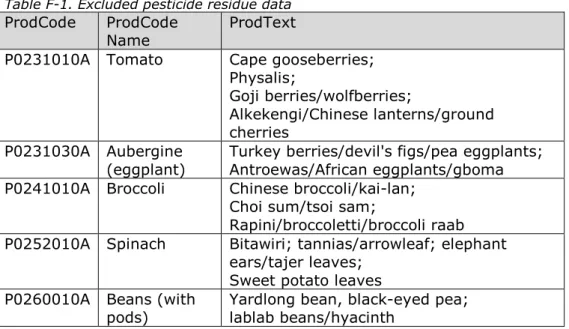
Based on additional information about the commodities analysed in the residue database, some results were excluded from the exposure 3_{Commission implementing Regulation (EU) 2015/595 of 15 April 2015 concerning a coordinated multiannual}

control programme of the Union for 2016, 2017 and 2018 to ensure compliance with maximum residue levels of pesticides and to assess the consumer exposure to pesticide residues in and on food of plant and animal origin; OJ L 99.

4_{Commission Regulation (EC) No 669/2009 of 24 July 2009 implementing Regulation (EC) No 882/2004 of the}

European Parliament and of the Council as regards the increased level of official controls on imports of certain feed and food of non-animal origin and amending Decision 2006/504/EC; OJ L 194.

5_{ec.europa.eu/food/safety/rasff_en}

6_{Regulation (EC) NO 396/2005 of the European Parliament and of the Council of 23 February 2005 on} maximum residue levels of pesticides in or on food and feed of plant and animal origin and amending Council Directive 91/414/EEC; OJ L 70.

(18)

assessment to avoid erroneous exposure results. These exclusions are described in Appendix F.

When the number of analysed samples for a substance/RAC combination with authorised use was less than 10, these samples were deemed to be too limited to represent the levels of the substance in the RAC as

available on the market. These analyses were therefore supplemented by concentration data of the same substance on another comparable RAC. This minimum number of 10 was in accordance with the FPA study. To supplement concentration data, the extrapolation principles for

treatments close to harvest were used as described in the EU guidelines on comparability, extrapolation, group tolerance and data requirements for setting maximum residue limits (MRLs) (EC, 2011). For this, it was assumed that the condition of good agricultural practice (GAP) similarity was satisfied when the MRL for the relevant substance/RAC combination was the same for the RAC(s) involved in the extrapolation. For the substance/RAC combinations for which no extrapolation could be performed, the concentration data as such were used in the exposure assessment. The extrapolations applied in this study were mainly related to the limited number of samples analysed for rye and oats. These samples were supplemented by those of wheat. For a limited number of substances, the measurements in wine grape and aubergines were supplemented by those in table grape and tomato, respectively. The residue data were expressed according to the legal residue definition for enforcement and monitoring, and used as such in the exposure assessment. Additionally, residue data of complex residue definitions covering more than one active substance were assumed to relate to the presence of the least potent of the authorised substances on the respective commodity (which can be a substance not included in the CAG) or to any eventual metabolite produced by these active substances when this metabolite is of lower potency. Footnotes per relevant substance in Appendices A, B, C and D indicate what this meant for this study.

The residue data were coded according to the Standard Sample

Description (SSD) format. According to this format, the RACs analysed are coded using the matrix code. This code is based on the coding used in Annex I of Regulation (EC) 396/2005, last amended by Regulation (EU) No 62/20187.

Appendices G, H, I and J provide an overview of the residue data of the substances belonging to the four CAGs.

2.5 Drinking water

A potential source of dietary exposure to residues of PPPs is drinking water (EFSA, 2012; Swartjes et al., 2016). This source of exposure should therefore also be considered in a cumulative exposure

assessment. As no residue data were available for drinking water, this source was considered by assuming that the five most potent

7_{Commission regulation (EC) No 2018/62 of 17 January 2018 replacing Annex I to Regulation (EC) No} 396/2005 of the European Parliament and of the Council; OJ L 18.

(19)

substances per CAG were present at a level of 0.05 µg/L. This level is equal to half the drinking water standard for individual residues of PPPs according to the Dutch Drinking Water Law8_.

One single water sample for each of the five substances per CAG was therefore added manually to the residue dataset. The substances for which this was done were

• carbofuran, methiocarb, formetanate, oxamyl and pirimicarb for the CAG-neurochemical;

• oxamyl, methiocarb, omethoate, fluquinconazole and cyfluthrin for the CAG-motor division;

• carbofuran , profenofos, ioxynil, ipconazole and fenamidone for the CAG-calcitonin;

• ioxynil, fipronil, propineb, amitrole and mepanipyrim for the CAG-thyroid hormone.

2.6 Linking foods analysed to those consumed

Residue data of PPP substances are predominantly analysed in raw agricultural commodities (RACs), whereas food consumption data are collected on foods as consumed. To link these two entities, the food conversion model delivered to EFSA in 2011 (Boon et al., Unpublished) was used. The basis for this food conversion model is the Dutch food conversion model (Boon et al., 2009; Geraets et al., 2011; van Dooren et al., 1995). This model was used because it converts foods coded at FoodEx1 (section 2.3) to RACs coded using the matrix code

(section 2.4). The food conversion model was extended to include consumed foods containing water as an ingredient (Appendix K). This was only done for consumed foods to which water was added ‘at home’, namely tea, coffee, lemonade and soup.

Some RACs (and drinking water) are consumed as such. This is, for example, the case for apples, pears and cucumbers. These RACs could therefore be linked directly to their consumed amounts as recorded in the food consumption databases. To also include the exposure via the consumption of processed and composite foods, such as apple juice, pizza and apple pie, the consumption of these foods was converted to equivalent consumptions of individual RACs. This was done based on recipe data and/or food conversion factors of processed ingredients to their raw counterparts. For example, pizza was first divided into

equivalent amounts of its ingredients, such as flour, onion and tomato, based on recipe data. These ingredients were subsequently converted to their raw counterparts (wheat, onion and tomato, respectively) using food conversion factors. Apple juice, which consists for 100% of apple, only the food conversion step was used to convert its consumption to its equivalent amount of raw apple. As part of the conversion also the processing type per RAC was identified to include possible effects of food handling on residues of PPPs in the exposure assessment (section 2.7). Apart from residue data in RACs, the residue database also contained some residue levels analysed in foods as consumed. These samples 8_{Richtlijn 98/83/EG van de Raad van 3 november 1998 betreffende de kwaliteit van voor menselijke}

(20)

could be linked directly to their consumed amounts as recorded in the food consumption survey. This was true for olive oil and wine. The consumption of foods for infants and young children (belonging to FoodEx 1 group A.17) could also be linked directly to analysed infant foods (Appendix L).

The residue database also contained concentrations of substances in fruit juices. These results were however not included in the exposure assessment, because the number of analysed samples was too limited. The exposure through the consumption of fruit juices was therefore included via the residue levels analysed in the raw fruits using the food conversion model. The same approach was followed for residues in some processed cereals which were also too limited for use in the assessment.

2.7 Effect of food handling on residue levels

RACs are typically consumed after some form of food handling, such as peeling or cooking. Concentrations of substances may be affected by this and therefore processing factors should be included in an exposure assessment when dealing with substances that are (predominantly) analysed in RACs and when the aim is to provide the most realistic exposure estimate possible. A processing factor is the ratio of the residue level in the processed commodity divided by the residue level in the raw commodity. Processing factors depend on food, processing type and substance.

In the present study, the same processing factors were used as those in the FPA study. These processing factors were exclusively collected from EFSA’s Reasoned Opinions9 covering the period until the end of July 2015. Additional processing factors were collected in this study for substance/RAC combinations that contributed largely to the cumulative exposure from EFSA conclusions on active substances, reports of the Joint FAO/WHO Meeting on Pesticide Residues (JMPR) published until September 2016 and the processing database of the German Federal Institute for Risk Assessment (BfR)10_.

Processing factors include both the effects from chemical alteration of the substance and from weight changes of the food (e.g. loss of water due to drying). However, the latter alterations relate to changes in the food itself and are already accounted for via the food conversion model (section 2.6). Processing factors were therefore corrected so that they only included the effect of processing on chemical alterations. For an example of such a correction, see Box 3.

9_{Reasoned opinions in application of Article 12 of Regulation (EC) No 396/2005 and subsequently further MRL} applications submitted for the respective active substance under Article 10 to the same regulation.

10_{Bundesinstitut für Risikobewertung (BfR) Data Collection on Processing Factors} http://www.bfr.bund.de/cm/349/bfr-compilation-of-processing-factors.xlsx

(21)

Box 3: Correction of processing factor for food conversion factor

The ratio of the presence of substance A in raisins to table grapes is 5 (= processing factor). In the food conversion model, the conversion factor of table grapes to raisins is 3.1. This means that you need 310 grams of table grapes to obtain 100 grams of raisins.

The corrected processing factor used in the exposure assessment will then equal 5

3.1 = 1.6.

An overview of the processing factors used in the present study is listed in Appendix D of the report of the FPA study.

2.8 Handling of left-censored data

Residue data of PPP substances often contain samples having an

analysed level below the limit of quantification (LOQ), the so-called left-censored samples. In these samples, it is not clear if the substance is present but at such a level that it cannot be quantified by the analytical method or that it is not present. To assign a concentration to these samples, preferably use frequency data are used. Use frequency data provide information about the expected presence of a substance on a RAC in a particular year and region, based on information about the use of PPPs by, for example, growers. Use frequency data can be used as follows. When these data suggest that a PPP containing the relevant substance may be used on 10% of the apples available on the market, 10% of the residue levels below LOQ in apple of this substance can be replaced with a specified level below the LOQ (e.g. ½LOQ), assuming that the substance is present. The remaining 90% of the residue levels below LOQ in apple can then equally be considered to not contain the substance based on these use data.

Unfortunately, use frequency data are not (readily) available. Therefore, the information available in the residue database was used to derive a ‘substitute’ use frequency per substance/RAC combination. Use

frequency was defined as the ratio of the samples having a quantifiable concentration of the substance and the total number of samples

analysed for this substance over the period of interest. Appendices M, N, O and P present an overview of the input parameters for the calculation of the use frequency per substance/RAC combination for the substances belonging to the four CAGs. Based on these use frequencies, either zero or a level equal to ½LOQ was assigned to the left-censored samples. Box 4 provides an example how this was done.

Box 4: Example of how residue levels were assigned to left-censored

samples.

Two out of the 249 analysed orange samples had a positive residue level for phosmet (Appendix E). The corresponding use frequency for this substance/RAC combination equalled therefore 0.008 (=2/249). Thus, the 247 remaining left-censored samples were assigned a zero

concentration with a probability of 99% and ½LOQ with a probability of 1%.

(22)

2.9 Missing values

Ideally, all samples analysed within a monitoring programme are

measured for all substances belonging to a CAG. In reality however, this is not true, and samples may have ‘missing values’. For example, 249 out of the 315 orange samples analysed in the period 2014-2016 were analysed for phosmet (Appendix G). To avoid underestimation of the exposure by assuming that these samples do not contain the substance, these missing values were also imputed based on the information on use frequencies (section 2.8). Imputation of the missing values was only performed for the acute CAGs: in a chronic assessment only a mean concentration per RAC/substance combination is needed (section 2.11).

2.10 Unit variability

Substances of PPPs are typically analysed in samples consisting of more than one unit of a RAC (e.g. apples are analysed in samples consisting of 12 units each). Because residue levels may vary between individual RAC units, consumers may be confronted with higher levels when consuming single units (e.g. one apple) than the average residue level analysed in a sample. To account for this possibility, unit variability factors are used in acute dietary exposure assessment. Unit variability is relevant for RACs having a unit weight larger than 25 grams (medium and large unit size). Examples of such RACs are apples, oranges, cauliflower and carrot.

To model the residue levels in individual units, information on the variability factor, unit weights of RACs and the number of units in a composite sample is needed.

Variability factors

A variability factor of 3.6 was used for all RACs having a unit weight larger than 25 grams. This variability factor is the average factor observed in market samples as reported in an opinion of EFSA’s PPR Panel on the use of the appropriate variability factor(s) for acute dietary intake assessment of pesticide residues (EFSA, 2005b).

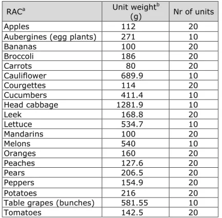
Unit weights

The unit weights of the EFSA PRIMo – Pesticide Residue Intake Model database (EFSA, 2018b), available at the EFSA website were used. Number of units in a sample

The number of units in an analysed sample was assumed to equal twice the minimum number as specified in the EU sampling Directive EC 2002/2311_{. This meant that the number of units equalled 20 for RACs} having a unit weight between 25 and 250 grams, and 10 for RACs having a unit weight above 250 grams.

For an overview of the unit weights and number of units in a sample used per RAC, see Appendix Q. Unit variability is only relevant for 11_{Commission Directive 2002/63/EC of 11 July 2002 establishingCommunity methods of sampling for the}

official control of pesticide residues in and on products of plant and animal origin and repealing Directive 79/700/EEC; OJ L 187.

(23)

calculating the exposure to the two CAGs covering acute effects on the nervous system.

2.11 Cumulative exposure assessment

Different methodologies are available to calculate the exposure to substances present in food, ranging from simple deterministic models (e.g. the EFSA Pesticide Residue Intake Model (PRIMo) used to assess the acute and chronic exposure to single residues of PPPs (EFSA, 2018b)) to probabilistic models. In deterministic models, summary statistics, such as a mean, median and/or high(est) level, of food consumption and concentration data are combined, resulting in a single estimate (typically, a mean or high level) of exposure. In probabilistic models, the whole food consumption and concentration database are used as input resulting in a distribution of exposure (Box 5). This distribution reflects the differences in exposure between individuals within a population due to differences in food consumption patterns and in residue levels within (acute) and between (acute and chronic) foods.

Box 5: Probabilistic modelling of dietary exposure

A probabilistic approach is needed to estimate the exposure to many substances via the consumption of many foods (EFSA, 2012). With this methodology, concentrations of different substances in many foods as well as correlations between concentrations of different substances in the same food sample are taken into account simultaneously. Also the consumption of many foods and correlations between foods consumed on a certain day (e.g., it is not likely that a person consumes endive and spinach on the same day, but may consume head cabbage in

combination with cucumber and tomato) are included. Deterministic models cannot consider all these input data at the same time in a meaningful way. In the EU 7th_{Framework project ACROPOLIS, a tool}

was developed to estimate cumulative exposure using a probabilistic approach (van der Voet et al, 2015), which has since been optimised further to make it suitable for assessing the cumulative exposure to large CAGs, consisting of up to a 100 substances (van der Voet et al., 2016). This tool is the Monte Carlo Risk Assessment (MCRA) software (release 8.2), which was used in this report for assessing the cumulative exposure to the four CAGs (de Boer et al., 2016; van der Voet et al., 2015; 2016).

(24)

The common toxic effects of the four CAGs included two acute effects on the nervous system and two chronic effects on the thyroid (section 2.1). Acute and chronic effects require the calculation of the acute and chronic exposure, respectively. Acute exposure relates to the exposure on an arbitrary day and, depending on the amounts of the relevant foods consumed and residue levels present in foods, can vary significantly from day to day within a person. Chronic exposure, on the other hand, relates to the average exposure over a longer period of time. In this type of assessment, variations in exposure between days within an individual are not relevant, as variations are expected to level out on the long-run.

The acute cumulative exposure was calculated by multiplying randomly drawn daily consumption patterns of foods from the food consumption database by randomly drawn sample based cumulative concentrations expressed in equivalents of the index compound (Box 2; section 2.2). This was done a 100.000 times. The resulting cumulative exposures per food per person-day were summed across foods resulting in a

distribution of 100.000 cumulative daily acute exposure estimates (Box 5).

The chronic cumulative exposure was calculated using the observed individual means (OIM) approach within MCRA. In this model, daily food consumption patterns of individuals obtained from the food consumption database were multiplied by the sample based mean cumulative residue level per food and summed over foods per day per individual.

Subsequently, the daily individual exposures were averaged over the two consumption days per individual, resulting in a distribution of two-day-average exposure levels per individual.

The exposure estimates were divided by the individual body weights. The exposure distributions of young children and persons aged 7 to 69 were furthermore weighted for small deviances in socio-demographic factors and season. The exposure distribution of this last age group was also corrected for day of the week12_{. The exposure distribution of the} persons aged 70+ were corrected for small differences in sex, age, region, level of urbanisation, day of the week and season as compared to the community-dwelling older Dutch adults. Weights were those used by Ocké et al. (2008; 2013) and van Rossum et al. (2011). For more detailed information about the cumulative exposure assessment within MCRA, see de Boer et al. (2016).

Information on use frequencies was used to assign zero or ½LOQ to left-censored samples (section 2.8), as well as to impute missing values (sections 2.9; Appendices M, N, O and P). Processing factors were included as a fixed factor by multiplying the factor by the relevant residue level per substance/RAC/processing combination (section 2.7). The effect of processing was included before calculating the cumulative concentration per analysed sample using RPFs (Box 2; section 2.2).

(25)

In the acute assessment, residue levels in single units were calculated based on the mean residue levels in analysed samples. This was done using the input data described in section 2.10, and assuming that the unit residue levels within an analysed sample follow a beta distribution. Using this distribution, it is assumed that the simulated unit residue levels are never higher than the residue level of the analysed sample times the number of units in the sample (i.e. the worst case is that one single unit contains all the substance within the sample). Unit variability was modelled for residue levels analysed in all RACs, except for those analysed in cereals, beans (with pods), olives (for oil production), peas (without pods), spinach, strawberry and wine grape. These RACs have a unit weight equal to or less than 25 grams.

The exposure was expressed in different percentiles of the cumulative exposure distribution, namely P50 (median), P90, P95, P99, P99.9 and P99.99 for four age groups: 2 to 6, 7 to 17, 18 to 69 and 70+ years. These age groups were selected to address possible differences in exposure, due to differences in food consumption patterns between age groups, and in consumption amounts per kg body weight. Young

children are, for example, known to have higher exposure levels than adults because of higher consumption levels per kg body weight. Also the contribution of the RACs, the substances and substance/RAC

combinations to the cumulative exposure were calculated per age group and CAG. In the FPA study, the exposure for the Netherlands was estimated for children aged 2 and children aged 3 to 6.

The uncertainty in the exposure due to the limited size of the food consumption and residue databases was calculated using the bootstrap approach. For more information about the bootstrap approach, see Box 6. The uncertainty was reported as the 95% confidence interval around the best estimates of the exposure percentiles. Such a

confidence interval means, considering the uncertainty addressed, that there is a 95% probability that the real exposure percentile falls within this interval, and thus that there is a 5% probability that the calculated percentiles may be outside the interval: 2.5% probability each that the real exposure percentile is lower or higher than the lower or upper limit of the confidence interval, respectively. The exposure was also

influenced by other sources of uncertainty. These are described and evaluated qualitatively according to the format proposed by EFSA (2006; 2012) in section 5.

(26)

Box 6: Bootstrap approach

To quantify the uncertainty in the exposure estimates due to the limited size of the food consumption and residue databases, the bootstrap approach can be used (Efron, 1979; Efron & Tibshirani, 1993). With this method, a bootstrap database is generated of the same size as the original database for both the food consumption and concentration database by sampling with replacement from the original datasets. These bootstrap databases are considered as databases that could have been obtained from the original population if another sample was

randomly drawn. These two bootstrap databases are then used for the exposure calculations and derivation of the relevant percentiles.

Repeating this process many times results in a bootstrap distribution for each percentile that allows for the derivation of confidence intervals around it. The bootstrap approach was used in this report by generating 100 food consumption and 100 concentration bootstrap databases and calculating the cumulative acute (with 10,000 iterations each) exposure. Of the resulting bootstrap distributions per percentile a 95% uncertainty interval was calculated by computing the 2.5% and 97.5% points of the empirical distribution.

Note that by bootstrapping both the consumption and concentration database in one analysis it is not possible to quantify which part of the uncertainty was due to a limited number of consumption or

(27)

3 Risk characterisation

To determine whether the calculated exposures could result in a potential health risk, a risk characterisation should be performed. For this, the calculated exposures are typically compared with a health-based guidance value (HBGV), such as the acceptable daily intake (ADI) for chronic exposure or acute reference dose (ARfD) for acute exposure, or a margin of exposure (MOE) is calculated. As guidance on how to perform a risk characterisation of cumulative exposure is not yet available, the MOE approach was used in this report. This approach provides a quantitative measure of the margin between a ‘safe intake level’ and the calculated exposure.

MOEs were calculated per CAG by dividing the NOAEL (‘safe intake level’) of the relevant index compound by the different percentiles of exposure (section 2.11). The NOAEL of oxamyl equalled 0.1 mg/kg bw for the CAGs covering effects on the nervous system (Appendices A and B). For the CAGs covering effects on the thyroid, the NOAELs for

fenbuconazole (CAG-calcitonin) and ioxynil (CAG-thyroid hormone) were 3 and 0.02 mg/kg bw, respectively (Appendices C and D). See Box 7 for an example how the MOE is calculated.

Box 7: Example of the calculation of a margin of exposure

The index compound of the CAG-neurchemical is oxamyl with a NOAEL of 0.1 mg/kg bw. Assuming that the P95 of exposure to this CAG equals 0.002 mg/kg bw per day, the margin of exposure (MOE) would equal

0.1

0.002= 50.

This means that the exposure to this CAG at the P95 level of the exposure distribution is 50 times lower than the NOAEL of the index compound.

The MOE can have the following outcomes: MOE = 1: the exposure equals the NOAEL

MOE < 1: the exposure is higher than the NOAEL MOE > 1: the exposure is lower than the NOAEL

The results of the exposure calculations, including the lower and upper limit of the 95% confidence interval, are expressed in MOEs.

(28)

(29)

4 Results

4.1 Two CAGs covering acute effects on the nervous system

4.1.1 CAG covering neurochemical effects

Margins of exposure

Table 1 lists the best estimates of the margins of exposure (MOEs) for the P99, P99.9 and P99.99 of dietary exposure for the CAG covering neurochemical effects, including the lower and upper limits of the 95% confidence interval. The MOEs of the percentiles of exposure up to the P95 were all higher than 500 (including those at the lower limit of the confidence interval). See Appendix R for an overview of the calculated MOEs.

The best estimates of the MOEs ranged from 31 in children aged 2 to 6 at the P99.99 to 1355 in the 70+ age group at the P99 (Table 1). Considering the quantified uncertainty in the estimated MOEs, the MOE could be as low as 280 for the P99, 54 for the P99.9 and 21 for the P99.99, all in the youngest age group (Table 1).

Table 1. Margins of exposure per exposure percentile for the CAG covering neurochemical effects

Age (years) Margins of exposure per exposure percentile

P99 P99.9 P99.99 2-6 396 (280 – 567) (54 – 181) 116 (21 -82) 31 7-17 881 (707 – 1245) (167 – 379) 254 (52 – 214) 109 18-69 1192 (998 – 1601) (166 – 571) 331 (74 – 285) 114 70+ 1355 (1058 – 1727) (89 - 536) 240 (39 – 225) 62

CAG: cumulative assessment group

Contribution RACs, substances and substance/RAC combinations to the upper 0.1% of the cumulative exposure distribution

As health risks related to the exposure to substances of PPPs

predominantly occur in the upper part of the exposure distribution, the contribution of the different parameters to the upper 0.1% of the acute cumulative exposure distribution to CAG-neurochemical was calculated. The cumulative exposure in this part of the exposure distribution was completely dominated by the consumption of spinach. The contribution of this commodity ranged from 30% in 7 to 17-year olds to up to 67% in young children and persons aged 70+. The substance contributing most to this upper part was pirimicarb in all age groups: 50 – 82%. The substance/RAC combination contributing was thus pirimicarb in spinach with contributions ranging from 30% to 67%. An important second contributor was the presence of methiocarb on beans (with pods) in the three older age groups: 24-25%. Other contributions of at least 10% were methiocarb in table grape (12%) and pirimicarb in strawberry

(30)

(11%) in children aged 7 to 17, and pirimicarb in apple (10%) in the youngest age group.

See Appendix S for an overview of the contribution of RACs, substances and substance/RAC combinations to the upper 0.1% of the exposure distribution per age group.

4.1.2 CAG covering effects on motor division

Margins of exposure

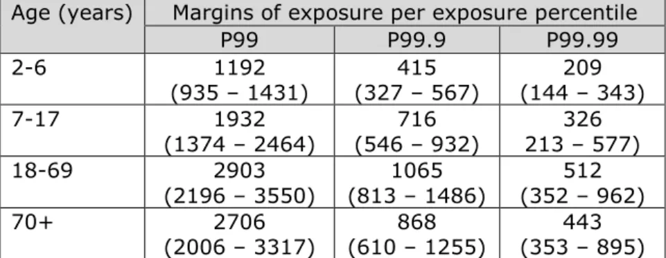
Table 2 lists the same information as Table 1, but now for the CAG covering effects on motor division. The MOEs of the percentiles of

exposure up to the P95 were all higher than 1500 (including those at the lower limit of the confidence interval). See Appendix R for an overview of the calculated MOEs.

The best estimates of the MOEs ranged from 209 in children aged 2 to 6 at the P99.99 to 2903 in the adult age group at the P99 (Table 2). Considering the quantified uncertainty in the estimated MOEs, the MOEs could be as low as 935 at the P99, 327 at the P99.9 and 144 at the P99.99, all in the youngest age group (Table 2).

Table 2. Margins of exposure per exposure percentiles for the CAG covering effects on motor division

P99 P99.9 P99.99 2-6 1192 (935 – 1431) (327 – 567) 415 (144 – 343) 209 7-17 1932 (1374 – 2464) (546 – 932) 716 213 – 577) 326 18-69 2903 (2196 – 3550) (813 – 1486) 1065 (352 – 962) 512 70+ 2706 (2006 – 3317) (610 – 1255) 868 (353 – 895) 443

Contribution RACs, substances and substance/RAC combinations to the upper 0.1% of the cumulative exposure distribution

The consumption of table grape, spinach, potato and beans (with pods) contributed more than 10% to the upper 0.1% of the acute cumulative exposure distribution in at least one of the age groups.

The dominant substance contributing to the upper 0.1% of the exposure distribution was lambda-cyhalothrin in all age groups with contributions ranging from 43% in the 7 to 17-year olds up to 66% in the oldest age group. Other substances that contributed for at least 10% were

deltamethrin (17%) and methiocarb (12%) in young children,

chlorpropham (11-25%) and methiocarb (11-13%) in children aged 7 to 17 and the adult age group, and deltamethrin (18%) in persons aged 70+.

Lambda-cyhalothrin in table grape, beans (with pods) and spinach, deltamethrin in spinach and chlorpropham in potato contributed at least 10% to the upper 0.1% of the cumulative exposure distribution in at least one of the age groups.

(31)

Appendix T provides an overview of the contribution of RACs,

substances and substance/RAC combinations to the upper 0.1% of the exposure distribution per age group.

4.2 Two CAGs covering chronic effects on the thyroid

Below we report on the MOEs of exposure for the CAGs covering chronic effects on the thyroid (Table 3). Since these MOEs were larger than 500, even at the highest calculated percentile (P99.99), contributions of the RACs to the upper part of the exposure distribution are not reported below. Also for these CAGs, the MOEs for the three highest percentiles of exposure were reported. See Appendix R for an overview of the calculated MOEs.

Table 3. Margins of exposure per exposure percentile for the CAGs covering effects on parafollicular (C-)cells or the calcitonin system on follicular cells and/or the thyroid hormone (T3/T4) system

P99 P99.9 P99.99 CAG-calcitonin 2-6 1729 (1445 – 1981) (922 – 1358) 1049 (726 – 1143) 903 7-17 3156 (2778 - 3484) (2139 – 2720) 2286 (1989 – 2597) 2092 18-69 2716 (2404 – 3045) (2004 – 2226) 2112 (1821 – 2196) 1929 70+ 3625 (3421 – 3916) (2806 – 3411) 2949 (2743 – 3264) 2791 CAG-thyroid hormone 2-6 6824 (4475 – 10270) (2151 – 5849) 3126 (2047 – 4625) 3054 7-17 12820 (9208 – 16840) (4695 – 11470) 7202 (4343 – 9369) 6043 18-69 17620 (11960 – 21590) (5410 – 15640) 10710 (3939 – 13240) 6118 70+ 17330 (11700 – 24090) (8047 – 18170) 13110 (7278 – 17180) 10580

The best estimates of the MOEs ranged from 903 at the P99.99 in the youngest age group to 3625 at the P99 in the 70+ age group for the CAG-calcitonin (Table 3). Corresponding numbers for CAG-thyroid

hormone were 3054 at the P99.99 in the youngest age group and 17620 at the P99 in the adult age group. Considering the quantified uncertainty in the estimated MOEs, the lowest MOEs for the CAG-calcitonin and CAG-thyroid hormone were 726 and 2047, respectively, for the P99.99 of exposure in the youngest age group.

(32)

(33)

5 Uncertainties in the cumulative exposure assessment

The cumulative exposure assessment of all four CAGs was influenced by different sources of uncertainty. The most important sources are

discussed in detail below.

5.1 Food consumption data

The food consumption data used in the cumulative exposure assessment were the most recent data available for the Netherlands (Appendix E). However, especially the food consumption data of children aged 2 to 6 were collected more than 10 years ago. Presently, a new food

consumption survey is being conducted among persons aged 1 to 79. Preliminary results of this survey collected in the period of 2012-2014 show that consumption patterns are changing13. A relevant change regarding this report is that the fruit consumption in children aged 7 to 18 has increased. However, the consumption of vegetables and cereals seems not to have changed since the previous food consumption survey. If the fruit consumption is indeed increased, in part or the total

population, the present estimates of exposure may underestimate the exposure to a certain extent. When the new data come available and confirm these changes in food consumption patterns, or show that also the consumption of vegetables and cereals has increased, it may be advisable to repeat the calculation. This would be most relevant for the CAG covering neurochemical effects, because the exposure to this CAG resulted in the lowest margins of exposure (Table 1).

Another important factor to take into account when estimating the exposure to substances present in food is that habitual eating patterns may be influenced or changed due to the recording process. Foods that are known to be healthy like fruits and vegetables may be eaten more on recording days than usually. If true, this may have resulted in an overestimation of the calculated exposure to residues of PPPs, which are mainly present in these healthy foods. The extent in which eating habits are changed due to the recording process and consequently the effect on calculated exposure levels is unknown. Another potential source of overestimation could have been the underreporting of body weight in the food consumption surveys. This source of overestimation is only relevant for the age group of 7 to 69: in the young children and 70+ surveys body weight was measured (Ocké et al., 2008; 2013; van Rossum et al., 2011). The extent in which body weights were underreported was not investigated (van Rossum et al., 2011).

To be in line with the FPA study, the FoodEx1 coding system was used to match foods consumed to those analysed. The FoodEx1 system is a less detailed coding system than the one of the Dutch Food Composition 13

www.rivm.nl/Onderwerpen/V/Voedselconsumptiepeiling/Overzicht_voedselconsumptiepeilingen/VCP_Basis_1_7 9_jaar_2012_2016

(34)

Database NEVO14, the food coding system that could also have been used in this study15. For vegetable products consumed as such, it is estimated that the error will be negligible as these foods are

predominantly coded at the highest (detailed) level of FoodEx1. For composite foods, this is less certain. FoodEx1 has only broad codes for composite foods and it can therefore not be ruled out that the use of the more detailed NEVO food codes would have resulted in a better match between the foods consumed and analysed. As less precise matching will typically result in more conservative estimates of exposure, because of conservative choices during linkage, the use of FoodEx1 may have resulted in an overestimation of the exposure.

5.2 Residue data

Monitoring data were used to calculate the cumulative exposure (section 2.4). By selecting only the samples that were randomly

sampled for inclusion in the exposure assessment, bias of the exposure to higher exposure levels was minimised as much as possible. However, despite this, it is generally known that monitoring data may not be representative of the foods available on the market and are likely to be biased to those commodities that are expected to contain PPP residues. Therefore, even though samples were not taken with any prior

knowledge of the presence of residues, overestimation of the exposure by using monitoring data cannot be ruled out completely. However, monitoring data are the best, and often the only data available for assessing the acute exposure, both to single and multiple substances. For acute exposure, residue levels per product are needed, making for example data of Total Diet Studies (TDS) not suitable for acute exposure assessment purposes (EFSA et al., 2011). TDS concentration data relate to foods as consumed and represent therefore potentially better the levels to which people are exposed than monitoring data. However, TDS data are average concentrations of substances in food, and therefore not suitable for use in an acute exposure assessment. For this type of

assessment, concentrations in individual foods are needed to reflect the daily variation in residue levels in foods (section 2.11). TDS data are however suitable to calculate chronic exposure, because for this type of exposure average residue levels per food are used (section 2.11). However, no TDS data on residues of PPPs were available for products available on the Dutch market.

In monitoring programmes, not all samples are analysed for all substances belonging to a CAG (section 2.9). Because this does not mean that the substance is not present, residue levels were assigned for the calculation of the cumulative sample concentration to minimise the possible underestimation of the exposure. Preferably, this should be based on knowledge about the actual use of PPPs, for example obtained from growers. As this information is not (readily) available, residue levels were assigned based on use frequency data per substance/RAC combination obtained from the residue database (section 2.8). Use frequency was defined as the number of samples with a positive residue 14_{nevo-online.rivm.nl/}

15_{The Dutch food consumption data are also coded at an ever more refined level than NEVO, namely by}

EPIC-Soft. However, these codes are not part of the Dutch food conversion model for mapping foods consumed to RACs.

(35)

level divided by the total number of samples analysed per

substance/RAC combination. As an alternative approach, it could have been assumed that residues were either not present or that they were always present at a certain positive level. This would very likely have resulted in either a very optimistic or conservative estimate of exposure, respectively. Using use frequency data, a more informed choice of presence or non-presence was possible, resulting in a better estimate of the exposure. The same was true for assigning a residue level to the samples with an analysed residue level below the limit of quantification (LOQ), the left-censored samples (section 2.8). Also here, the

assumption could have been that these samples do either not contain the residue or the residue is present at (a fraction of the) LOQ, instead of using use frequency data to assign a residue level. As PPPs are not used on all commodities available on the market, the latter option would again have resulted in a conservative exposure estimate, whereas assuming that all left-censored samples do not contain the residue would have been too optimistic. How well the use frequency data used in this study reflect the real use frequency data of PPPs in the field is very uncertain, as no information is available. This approach could have resulted in a under- or overestimation of the exposure. Availability of information about the use of PPPs by for example growers will reduce this uncertainty.

In this assessment, 30 RACs were included. These 30 RACs formed the majority of the vegetable products consumed in the Netherlands,

including for example apple, potato, wheat, cauliflower, carrot, etc. This selection is therefore judged not to have resulted in an underestimation of the cumulative exposure to all four CAGs.

Another source of uncertainty related to the residue data were the residue levels in drinking water. As no monitoring data were available for this source and exposure via drinking water cannot be excluded (EFSA, 2012; Swartjes et al., 2016), possible exposure via drinking water was considered using an assumed presence of five substances per CAG at 0.05 µg/L (section 2.5). This is equal to half the drinking water standard for single residues of PPPs according to the Dutch Drinking Water Law. The sum of the single residues should not exceed 5 µg/L according to this law. Based on a Dutch study into the presence of residues of PPPs in groundwater resources of drinking water wells (Swartjes et al., 2016), the assumption about the presence of residues in drinking water in this study has very likely resulted in an

overestimation of the exposure via drinking water. Use of analytical data will reduce this source of uncertainty.

In a cumulative risk assessment, the potential contribution of

metabolites and degradation products to the specific effects should be taken into account (EFSA, 2018a). As information of residue definitions of active substances related to the common effect is lacking, the residue definition of enforcement and monitoring was used, as in the FPA study. To assess whether this has resulted in an over- or underestimation of the cumulative exposure per CAG, the residue definitions per substance should be examined in relation to the same toxic effect in the organ. Additionally, residue data referring to complex residue definitions for enforcement and monitoring were assumed to relate to the presence of

(36)

the least potent authorised substance or metabolite produced (section 2.4). This is a potential source of underestimation of the exposure to the four CAGs like in the FPA study. As the number of substances with a complex residue definition was limited for the CAG-neurochemical and CAG-calcitonin (Appendices A and C), the effect on the exposure to these two CAGs is expected to be limited. For the other two CAGs, the number of substances with a complex residue definition was however larger (Appendices B and D). An underestimation of the exposure to these two CAGs is therefore likely.

5.3 Processing and modelling unit variability

In this assessment, the same processing factors were used as in the FPA study. The information on the effect of processing was very limited, because of the large number of possible substance/RAC/processing types combinations included in the exposure assessment of the four CAGs. For example, there was no processing information available for pirimicarb in spinach and methiocarb in beans (with pods), important contributors to the exposure to the CAG-neurochemical; the CAG with the lowest margins of exposure (section 4.1.1). For pirimicarb in apple, an important contributor to the exposure in young children for this CAG, processing factors were present for the processing types ‘sauce / puree’ (0.5) and ‘juicing’ (0.745). However, the majority of apple consumed in this age group was raw (with or without peel). As processing mainly results in a decrease of the residue levels in the processed food compared to the raw product, except for processing types in which commodities are concentrated (e.g. drying and oil extraction), including processing only to a limited extent in the assessment will have resulted in an overestimation of the exposure.

In the present assessment, a mean variability factor of 3.6 was used as observed in market samples (section 2.10). The EFSA guidance on probabilistic modelling does not give direction on which variability factor to use in an acute probabilistic exposure assessment using monitoring data (EFSA, 2012). In deterministic approaches to estimate acute exposure to single compounds, EFSA uses five and seven (EFSA, 2018b), whereas JMRR uses three (FAO/WHO, 2017). Based on the information available, a variability factor of 3.6 was estimated to reflect best the true variability within samples obtained in monitoring

programmes. Boon et al. (2015) estimated the cumulative exposure to a selected group of residues of PPPs of the triazole group for a number of European countries according to EFSA guidance on probabilistic

modelling. In that study, a variability factor of five was used, and the authors argue that because this factor is higher than the one observed in market samples, that the true proportion of single units with high residue levels was very likely overestimated.

5.4 Linking foods analysed to those consumed

The foods analysed were linked to those recorded in the food

consumption database, either via a food conversion model or directly (section 2.6).

Linking of foods is a large source of uncertainty in an exposure

(37)

consumed. Residues of PPPs are analysed in raw agricultural

commodities (RACs) within monitoring programmes to establish whether commodities comply with maximum residue limits. These analyses are performed as part of different monitoring obligations prescribed in legislation and therefore available every year. However, when using these data, a food conversion model is needed to include all relevant foods consumed (including processed and composite foods) in the assessment. Without this model, only the foods consumed as RAC can be included, resulting in an underestimation of the exposure. So for example, the exposure via apple consumption could be included, but not that via the consumption of apple pie and apple juice.

Advantage of such a model is that concentrations analysed in RACs are linked to consumed amounts of composite foods, which contain these RACs as ingredient, or of processed foods consisting of a single RAC ingredient (e.g. cooked cauliflower, frozen spinach) (section 2.6). These foods are thus included in the assessment without the need to analyse them separately. A disadvantage of this approach is that there is no direct link between analysed and consumed foods. As a result, there is always an uncertainty whether the calculated concentrations in

consumed foods via the food conversion model are representative for the concentrations in those actually consumed. The residue database contained some data in foods as consumed (section 2.6). The number of samples was however too limited for fruit juices and some processed cereals. These data were therefore not included in the assessment. The residue levels present in these foods estimated via those analysed in the corresponding RACs and the food conversion model. Increasing the number of analyses of these foods could result in a better estimate of the residue levels in these foods.

An additional uncertainty related to the use of residue levels in RACs and the use of the food conversion model is the change in the

composition of food products over time. The food conversion model was generated in 1995 and has since then only been updated by including additional food products recorded in the ensuing food consumption surveys. The composition of the already included food products has not been updated and therefore the composition may no longer be

representative for all relevant foods currently on the market.

Furthermore, recipes in the conversion table were based on information from cook books, food act, literature, label of the food, internet or manufacturer (van Dooren et al., 1995), resulting in one typical recipe per food. Variations in recipes were not addressed. This was also true for the conversion factors within the conversion model.

Considering these uncertainties, using concentrations analysed in RACs may have resulted in over- or underestimates of the exposure. However, considering the large number of foods included, overall the uncertainties may have levelled out in the final exposure estimates.

5.5 Exposure assessment

The cumulative exposure was performed largely in accordance to the 2012 EFSA guidance on the use of the probabilistic methodology for modelling dietary exposure to residues of PPPs (EFSA, 2012). In this