Space Weather Training Course

(1)

Hullie

(2)

(3)

(4)

The Sun is a star Radiating 3,84 * 1026_Watt = 1362 W/m2_{at Earth} Big 1.392.000 km (109 * D_E) Heavy 1,99 * 1030_{kg (332.980 * M} E) Closest star 149.597.870 km = 1 Astronomical Unit The solar interior:

Core (R = +/- 175.000 km)

Energy production (proton-proton cycle) Radiation zone (325.000 km)

Energy transport thru radiation Convection zone (200.000 km)

Energy transport thru convection The solar atmosphere

Photosphere

The “solar surface” ; The Sun in visible light Chromosphere (very thin)

Prominences The Corona

The Sun’s outer atmosphere, as visible during a solar eclipse Very hot!

(5)

Links

SILSO: http://sidc.oma.be/silso/ (Sunspot Index and Long-term Solar Observations) USET: http://www.sidc.be/uset/ (Uccle Solar Equatorial Table)

Catania: http://web.ct.astro.it/sun/draw.jpg

The International sunspot number is a quantity that measures the number of sunspots and groups of sunspots present on the surface of the sun.

It is computed from a number of international observers using the formula: R = k ( 10 g + s )

where

s is the number of individual spots, g is the number of sunspot groups, and

k is a factor that varies with location and instrumentation (also known as the observatory factor or the personal reduction coefficient). It is not to be computed or applied by the observer.

(6)

Links

SILSO: http://sidc.oma.be/silso/ (Sunspot Index and Long-term Solar Observations) USET: http://www.sidc.be/uset/ (Uccle Solar Equatorial Table)

Catania: http://web.ct.astro.it/sun/draw.jpg

The International sunspot number is a quantity that measures the number of sunspots and groups of sunspots present on the surface of the sun.

It is computed from a number of international observers using the formula: R = k ( 10 g + s )

where

s is the number of individual spots, g is the number of sunspot groups, and

k is a factor that varies with location and instrumentation (also known as the observatory factor or the personal reduction coefficient). It is not to be computed or applied by the observer.

(7)

(8)

More info at http://aia.lmsal.com/public/instrument.htm

(9)

Lagrangian points: https://en.wikipedia.org/wiki/Lagrangian_point

Earth orbits: https://en.wikipedia.org/wiki/List_of_orbits#Altitude_classifications_for_geocentric_orbits * GEO: GOES, SDO (inclined)

Advantages and disadvantages of SDO in GEO at https://sdo.gsfc.nasa.gov/mission/project.php

Orbit

The rapid cadence and continuous coverage required for SDO observations led to placing the satellite into an inclined geosynchronous orbit. This allows for a nearly-continuous, high-data-rate, contact with a single, dedicated, ground station.

Nearly continuous observations of the Sun can be obtained from other orbits, such as low Earth orbit (LEO). If SDO were placed into an LEO it would be necessary to store large volumes of scientific data onboard until a downlink opportunity. The large data rate of SDO, along with the difficulties in managing a large on-board storage system, resulted in a requirement of continuous contact.

The disadvantages of this orbit include higher launch and orbit acquisition costs (relative to LEO) and eclipse (Earth shadow) seasons twice annually, During these 2-3 week eclipse periods, SDO will experience a daily interruption of solar observations. There will also be three lunar shadow events each year from this orbit. This orbit is located on the outer reaches of the Earth's radiation belt where the radiation dose can be quite high. Additional shielding was added to the instruments and electronics to reduce the problems caused by exposure to radiation. Because this is a Space Weather effect, SDO is affected by the very processes it is designed to study!

(10)

(11)

(12)

(13)

(14)

Text from the CISM Summer School (Boulder, August 2013) – SW101_4_Flares https://www.bu.edu/cism/SummerSchool/summerlist.html

Right animation from ESA: http://sci.esa.int/cluster/36447-direct-observation-of-3d-magnetic-reconnection/

(15)

(16)

(17)

From the CISM Summer School (Boulder, August 2013) – SW101_4_Flares https://www.bu.edu/cism/SummerSchool/summerlist.html

Solar flares are sudden bursts of radiation lasting minutes – hours at wavelengths that can include: Gamma-rays, HXR, SXR, EUV; H-alpha, radio

A large quantity of energy is released from a small volume in a short period of time. This requires: Either a large amount of energy stored in that small volume that can be quickly transformed and released as energetic electrons and photons.

Or very efficient transport of energy into that volume where it is then converted into the observed forms.

The only viable energy source is intense solar magnetic fields.

Thus we need a very rapid means of converting stored magnetic energy into particle energy and heat – magnetic reconnection.

Magnetic energy is converted to thermal/radiative energy (flare, radio bursts) and

kinetic energy (mass movement from CMEs and SEPs).

http://solarphysics.livingreviews.org/Articles/lrsp-2011-6/ Solar Flares: Magnetohydrodynamic Processes

Kazunari Shibata and Tetsuya Magara

Solar flares are explosive phenomena observed in the solar atmosphere filled with magnetized plasma.

Flares are observed in a wide range of electromagnetic waves such as radio, visible light, X-rays, and gamma rays.

(18)

Magnetic flux emergence: X6.9 flare on 9 August 2011: http://www.stce.be/news/353/welcome.html Blue/black is negative (inward) magnetic polarity, red/white is positive (outward) polarity

(19)

http://www.stce.be/news/157/welcome.html http://www.stce.be/news/218/welcome.html

(20)

http://www.stce.be/news/362/welcome.html

Mason et al. (2016): Relationship of EUV Irradiance Coronal Dimming Slope and Depth to Coronal Mass Ejection Speed and Mass

http://adsabs.harvard.edu/abs/2016ApJ...830...20M

Large regions of temporary dimming or darkening of preexisting solar coronal emission often accompany coronal mass ejections (CMEs) and may trace field lines opened during the CME. The plasma of the solar corona responds in a number of ways to an eruptive event. Mason et al. (2014) provide details about the physics behind coronal dimming and the observational effects to be considered during analysis. Therein, the case is made for two hypotheses: that the slope of de-convolved, extreme-ultraviolet (EUV) dimming irradiance light curves should be directly proportional to CME speed, and similarly, that dimming depth should scale with CME mass. Dimming regions can be extensive, representing at least part of the “base” of a CME and the mass and magnetic flux transported outward by it.

Extensive surveys of EUV images containing coronal dimming events and their relation to CMEs have been performed by Reinard & Biesecker (2008, 2009). For their sample of 100 dimming events, Reinard & Biesecker (2008) found mean lifetimes of 8 hr, with most disappearing within a day. Reinard & Biesecker (2009) studied CMEs with and without associated dimmings, finding that those with dimmings tended to be faster and more energetic. Bewsher et al. (2008) found a 55%

association rate of dimming events with CMEs and conversely that 84% of CME events exhibited dimming.

The timescale for dimming development is typically several minutes to an hour. This is much faster than the radiative cooling time, which implies that the cause of the decreased emission is more dependent on density decrease than temperature change (Hudson et al. 1996). Studies have demonstrated that dimming regions can be a good indicator of the apparent base of the white light CME (Thompson et al. 2000; Harrison et al. 2003; Zhukov & Auchère 2004). Thus, dimmings are usually interpreted as mass depletions due to the loss or rapid expansion of the overlying corona (Hudson et al. 1998; Harrison & Lyons 2000; Zhukov & Auchère 2004).

(21)

Source: http://iopscience.iop.org/article/10.1086/304521/fulltext/36016.text.html From SWPC ’s « The Weekly » User guide

(https://www.swpc.noaa.gov/sites/default/files/images/u2/Usr_guide.pdf ; page 2)

The letter classification of solar flares used in these definitions (Table 1) was initiated on 01 January 1969. This classification ranks solar activity by its peak x-ray intensity in the 0.1-0.8 nm band as measured by the Geostationary Operational Environmental Satellites (GOES). This x-ray classification offers at least two distinct advantages compared with the standard optical classifications: it gives a better measure of the geophysical significance of a solar event, and it provides an objective means of classifying geophysically significant activity regardless of its location on the solar disk.

Table 1. The SWPC x-ray flare classification Peak Flux Range (0.1-0.8 nm)

Classification mks system (W m-2) cgs system (erg cm-2s-1)

A Φ <10-7 Φ <10-4

B 10-7 ≤ Φ <10-6 10-4 ≤ Φ <10-3 C 10-6 ≤ Φ <10-5 10-3 ≤ Φ <10-2 M 10-5 ≤ Φ <10-4 10-2 ≤ Φ <10-1

X 10-4 ≤ Φ 10-1 ≤ Φ

The letter designates the order of magnitude of the peak value and the number following the letter is the multiplicative factor. A C3.2 event for example, indicates an x-ray burst with 3.2x10-6Wm-2 peak flux. Solar flare forecasts are usually issued only in terms of the broad C, M, and X categories. Since x-ray bursts are observed as a full-Sun value, bursts below the x-ray background level are not discernible. The background drops to class A level during solar minimum; only bursts that exceed B1.0 are classified as x-ray events. During solar maximum the background is often at the class M level, therefore class A, B, or C x-ray bursts cannot be discerned. Data are measured by the NOAA GOES satellites, monitored in real time in Boulder (Grubb 1975).

---

(22)

Source: http://iopscience.iop.org/article/10.1086/304521/fulltext/36016.text.html

X-ray Background: The daily average background x-ray flux as measured by the GOES satellite. To better reflect mid day values, the average is the lower of (a) the average of 1-minute data between 0800UT to 1600UT, or (b) the average of the 0000UT to 0800UT and the 1600UT to 2400UT data. The value is given in terms of x-ray class (Donnelly 1982); (Bouwer, et al.1982). X-ray flux values below the B1 level can be erroneous because of energetic electron contamination of the x-ray sensors. At times of high electron flux at geosynchronous altitude, the x-ray measurements in the low A-class range can be in error by 20-30 percent. Measurements taken during periods of low energetic electron fluxes are much more accurate.

Barbara Poppe – Sentinels of the Sun (2006) – pp. 120

First, ¡n the mid-1960s Don Baker classified solar flares using x-ray data. The Naval Research Laboratory used German-made Vela V2 rockets, captured by the Americans after the war, to measure x-rays from the Sun. Baker, then working at the Space Disturbances Laboratory (SDL), used these data to identify the wavelengths, 1 to 8 angstroms, that best characterized a flare’s intensity. He created NOAA’s flare classification, labeled “CMX”: C, M, and X stand for

small, medium, and large flares, with a range within each category from 1 to 9 (e.g., an M1 flare is one step higher than a C9 flare). Having C represent the smallest flare left A and B open should there be observations smaller than those currently known. Similarly, Y and Z could follow X ¡f scientists discovered extremely large flares. A and B flares can now in fact be seen with improved

instrumentation and are categorized as such. Y and Z have never been used, despite the orderly progression that should have followed as scientists classified bigger and bigger Hares (an X1 to X9 would be followed by Y1 to Y9, then Z1 to Z9). Instead we have now seen an X28 flare. This classification system replaced an older one that reported flux numbers; that is, the flare is an M5 rather than flux Φ = 5 x 10^(-5) watts/m2. The improvement was obvious.

(23)

Source: https://www.swpc.noaa.gov/sites/default/files/images/u2/Usr_guide.pdf Solar Activity in SC24 (Jan 2009 - Dec 2016)

(24)

From the SWPC webpage: NOAA Space Weather Scales

The NOAA Space Weather Scales were introduced as a way to communicate to the general public the current and future space weather conditions and their possible effects on people and systems. Many of the SWPC products describe the space environment, but few have described the effects that can be experienced as the result of environmental disturbances. These scales are useful to users of our products and those who are interested in space weather effects. The scales describe the

environmental disturbances for three event types: geomagnetic storms, solar radiation storms, and radio blackouts. The scales have numbered levels, analogous to hurricanes, tornadoes, and

earthquakes that convey severity. They list possible effects at each level. They also show how often such events happen, and give a measure of the intensity of the physical causes.

The « R » stands for Radio Blackout. Note it starts only from M1 class flares and higher. More at http://www.stce.be/news/366/welcome.html

(25)

The « R » stands for Radio Blackout. Note it starts only from M1 class flares and higher. More at http://www.stce.be/news/366/welcome.html

Systematic satellite observations of the Sun started in 1976 with GOES. For each year and for each disturbance type, one can count for every level the number of events. E.g. so far for 2016, we've had only 10 R1 events (flares with intensity between M1 and M5) and 4 R2 events (intensity between M5 and X1). Data can be retrieved at resp. NGDC/NOAA, NASA/NOAA and WDC Kyoto, and run through mid-October 2016.

Each graph shows the yearly accumulation of the events, with the yearly International Sunspot Number (SILSO) superposed on it as the gray dashed line. E.g. in the chart above, for 2014 -the year of SC24 maximum-, the number of radio blackouts amounted to 222, consisting of 183 minor (R1), 23 moderate (R2), and 16 strong (R3) events. This is clearly less than during previous solar cycles such as e.g. in 1989 when there were no less than 679 radio blackouts including 59 strong or more intense events! Also, SC24 has not produced any severe or extreme event so far, i.e. X10 or stronger flare.

(26)

From Notsu et al. (2019): « Do Kepler Superflare Stars Really Include Slowly Rotating Sun-like Stars? – Results Using APO 3.5m Telescope Spectroscopic Observations and Gaia-DR2 Data » , https://iopscience.iop.org/article/10.3847/1538-4357/ab14e6 ; https://doi.org/10.3847/1538-4357/ab14e6

Figure 17. Comparison between the frequency distribution of superflares and solar flares. The red square, blue dashed line, and blue open squares indicate the occurrence frequency distributions of superflares on Sun-like stars (slowly rotating solar-type stars with Teff = 5600–6000 K). The red square corresponds to the updated frequency value of superflares on the stars with Prot = 20–40 days, which are calculated in this study and presented in Figure 16. Horizontal and vertical error bars are the same as those in Figure 16. For reference, the blue dashed line and blue open squares are the values of superflares on the stars with Prot > 10 days, which we presented in Figure 4 of Maehara et al. (2015) on the basis of original superflare data using Kepler 30-minute cadence data (Shibayama et al. 2013) and 1-minute cadence data (Maehara et al. 2015), respectively. Definitions of error bars of the blue open squares are the same as those in Figure 4 of Maehara et al. (2015). Three dashed lines on the upper left side of this figure indicate the power-law frequency distribution of solar flares observed in hard X-ray (Crosby et al. 1993), soft X-ray (Shimizu 1995), and EUV (Aschwanden et al. 2000). Occurrence frequency distributions of superflares on Sun-like stars and solar flares are roughly on the same power-law line with an index of −1.8 (black solid line) for the wide energy range between 1024 and 1035 erg.

It might be better to use only the data of stars rotating as slowly as the Sun (Prot ~ 25 days and t ~ 4.6 Gyr). Then, in Figure 17 we newly plot the frequency value of superflares on Sun-like stars with Prot = 20–40 days (t > 3.2 Gyr) taken from Figure 16, in addition to the data of solar flares and superflares shown in Figure 4 of Maehara et al. (2015). As a result, the newly added data point of superflares on Sun-like stars is roughly on the same power-law line, though the exact value of superflare frequency of stars with Prot = 20–40 days (t > 3.2 Gyr) is a bit smaller than those of stars with Prot > 10 days (t > 1 Gyr). From this figure, we can roughly remark that superflares with energy >1034 erg would be approximately once every 2000–3000 yr on old Sun-like stars with Prot ~ 25 days and t ~ 4.6 Gyr, though the error value is relatively large because of the small amount of data of slowly rotating stars.

Wikipedia (https://en.wikipedia.org/wiki/Superflare ) summarizes it as follows: An estimate based on the original Kepler photometric studies suggested a frequency on solar-type stars (early G-type and rotation period more than 10 days) of once every 800 years for an energy of 1034 erg and every 5000 years at 1035 erg. One-minute sampling provided statistics for less energetic flares and gave a frequency of one flare of energy 1033 erg every 5–600 years for a star rotating as slowly as the Sun; this would be rated as X100 on the solar flare scale. … There is no evidence for any flare greater than the Carrington event (about 1032 erg, or 1/10,000 of the largest superflares) in the last 200 years. … The more energetic superflares seem to be ruled out by energetic considerations for our sun, which suggest it is not capable of a flare of more than 1034 ergs. A calculation of the free energy in magnetic fields in active regions that could be released as flares gives a lower upper bound of around 3×1032 erg suggesting the most energetic a super flare can be is three times that of the Carrington event.

(27)

NASA: Hinode Discovers the Origin of White Light Flare (2010)

https://www.nasa.gov/centers/marshall/news/news/releases/2010/10-052.html

White light emissions were observed by the Solar Optical Telescope during an X-class flare that occurred at 22:09 UT on Dec. 14, 2006 (see Fig. 1). The RHESSI satellite simultaneously recorded hard X-ray emissions, an indicator of non-thermal electrons accelerated by solar flares. The team found that the spatial location and temporal change of white light emissions are correlated with those of hard X-ray emissions (see Fig. 2). Moreover, the energy of white light emissions is equivalent to the energy supplied by all the electrons accelerated to above 40 keV (~40 percent of the light speed). This finding strongly suggests that highly accelerated electrons are responsible for producing white light emissions.

Hard X-rays are emitted when accelerated electrons impact the dense atmosphere near the solar surface. Normally, white light emissions primarily come from the solar surface, whereas 40 keV electrons can penetrate into the atmosphere about 1,000 km above the solar surface, i.e., the chromosphere.

Fig. 1, above, White light images of solar surface observed by the Hinode Solar Optical Telescope at 22:07 UT, before the flare, and below, at 22:09 UT, during the flare on Dec. 14, 2006. Image Credit: NASA/JAXA

Fig.2: White light emission, left, taken by Hinode/SOT, and the difference image of white light emission and RHESSI hard X-ray contours at 22:09 UT. The background image is the differential white light image (the average of the images taken at 22:07 UT and 22:17 UT is subtracted). Blue contours show 40-100 keV emission. Image credit: NASA/JAXA

An overview of WLFs is at http://users.telenet.be/j.janssens/WLF/Whitelightflare.html (last update: August 2012).

(28)

Source of Figure: SWPC ’s « The Weekly » User guide

(https://www.swpc.noaa.gov/sites/default/files/images/u2/Usr_guide.pdf ; page 5)

Mind the orientation of the vertical axis! Other figures may have a reversed direction. As the frequency is proportional to the square root of the density, and the density decreases with increasing distance from the Sun, a decreasing frequency means locations higher up in the solar atmosphere.

The ionospheric cut-off frequency is around 15MHz (due to too low frequency and so reflected by ionosphere). In order to observe radio disturbances below this frequency, one has to use satellites (above the earth atmosphere) such as STEREO/SWAVES or WIND. Radio bursts at low frequencies (< 15 MHz) are of particular interest because they are associated with energetic CMEs that travel far into the interplanetary (IP) medium and affect Earth’s space environment if Earth-directed. Low frequency radio emission needs to be observed from space because of the ionospheric cutoff.

Example: https://stereo-ssc.nascom.nasa.gov/browse/2017/01/16/insitu.shtml Solar Radio Bursts and Space Weather, S.M. White

https://www.nrao.edu/astrores/gbsrbs/Pubs/AJP_07.pdf

White: Solar radio bursts at frequencies below a few hundred MHz were classified into 5 types in the 1960s (Wild et al., 1963).

Coronal Mass Ejections and solar radio emissions, N. Gopalswamy

http://citeseerx.ist.psu.edu/viewdoc/download?doi=10.1.1.708.626&rep=rep1&type=pdf

Gopalswamy: The three most relevant to space weather radio burst types are type II, III, and IV. Three types of low-frequency non-thermal radio bursts are associated with coronal mass ejections (CMEs): Type III bursts due to accelerated electrons propagating along open magnetic field lines, type II bursts due to electrons accelerated in shocks, and type IV bursts due to electrons trapped in post-eruption arcades behind CMEs.

(29)

(30)

(31)

SWPC ’s « The Weekly » User guide (https://www.swpc.noaa.gov/sites/default/files/images/u2/Usr_guide.pdf ; page 15) Proton Events

A proton event starts when the integrated proton flux (5-minute average) rises above a specific threshold for at least three points.

The two alert thresholds are (1 pfu = particle / cm-2s-1sr-1): - >10 MeV: ≥10 pfu

- >100 MeV: ≥ 1 pfu

The time of maximum is the time tag of the 5 minute averaged flux value that has the greatest value. The term « proton flare » is also commonly used. According to the SWPC glossary at

https://www.swpc.noaa.gov/content/space-weather-glossary , a proton flare is « Any flare producing significant counts of protons with energies exceeding 10 MeV in the vicinity of the Earth. »

Because proton events can originate from eruptions on the Sun’s farside, i.e. without a flare recorded by GOES, proton flares are a subset of proton events.

From: http://www.stce.be/news/232/welcome.html

The issue here is that proton flares are not considered as separate events if the proton flux (particle energies larger than 10 MeV) at the time of the event is still above the threshold of 10 protons per flux unit (pfu). Example: 6 January 2014 X1 proton flare.

From: SESC: https://umbra.nascom.nasa.gov/SEP/ (contains list of all proton events since 1976)

Please Note: Proton fluxes are integral 5-minute averages for energies >10 MeV, given in Particle Flux Units (pfu), measured by GOES spacecraft at Geosynchronous orbit: 1 pfu = 1 p / cm-2_sr-1_s-1_{. SESC defines the start of a proton event to be the first of 3} consecutive data points with fluxes greater than or equal to 10 pfu. The end of an event is the last time the flux was greater than or equal to 10 pfu. This definition, motivated by SESC customer needs, allows multiple proton flares and/or interplanetary shock proton increases to occur within one SESC proton event. Additional data may be necessary to more completely resolve any individual proton event.

SEP definition: from SWPC’s glossary

https://www.swpc.noaa.gov/content/space-weather-glossary#Solar%20Energetic%20Particles

(32)

From the SWPC webpage (https://www.swpc.noaa.gov/noaa-scales-explanation ) NOAA Space Weather Scales

The « S » stands for Solar radiation Storm. Since observations started in 1976, no S5 event has been recorded.

(33)

From the SWPC webpage (https://www.swpc.noaa.gov/noaa-scales-explanation ): NOAA Space Weather Scales

More on NOAA scales at http://www.stce.be/news/366/welcome.html More on proton intensity at http://www.stce.be/news/233/welcome.html

(34)

From the SWPC webpage (https://www.swpc.noaa.gov/noaa-scales-explanation ) NOAA Space Weather Scales

(35)

(36)

(37)

Figure to the right taken from https://ase.tufts.edu/cosmos/print_images.asp?id=27

A magnetic reconnection takes place at a current sheet (dark vertical line) beneath a prominence and above closed magnetic field lines. The coronal mass ejection, abbreviated CME, traps hot plasma below it (hatched region). The solid curve at the top is the bow shock driven by the CME. The closed field region above the prominence (center) is supposed to become a flux rope in the interplanetary medium. [Adapted from Petrus C. Martens and N. Paul Kuin (1989).]

In this model of a three-part coronal mass ejection, portrayed by Terry Forbes (2000), swept-up, compressed mass and a bow shock have been added to the eruptive-flare portrayal of Tadashi Hirayama (1974). The combined representation includes compressed material at the leading edge of a low-density, magnetic bubble or cavity, and dense prominence gas. The prominence and its surrounding cavity rise through the lower corona, followed by sequential magnetic reconnection and the formation of flare ribbons at the footpoints of a loop arcade. [Adapted from Hugh S. Hudson, Jean-Louis Bougeret and Joan Burkepile (2006).]

Figure to the left taken from Forbes (2000): A review on the genesis of coronal mass ejection http://adsabs.harvard.edu/abs/2000JGR...10523153F

http://onlinelibrary.wiley.com/doi/10.1029/2000JA000005/epdf

When CMEs were first clearly identified by Skylab in 1973, many researchers assumed that they were caused by the outward expansion of hot plasma produced by a large flare. We now know that this is not the case, for several reasons. First, less than 20% of all CMEs are associated with large flares [Gosling, 1993]. Second, CMEs that are associated with flares often appear to start before the onset of the flare [Wagner et al., 1981; Simnett and Harrison, 1985]. Finally, the thermal pressure produced by a flare is too small to blow open the strong magnetic field of the corona.

(38)

Expanding flux rope consisting of magnetic field lines and filament at bottom evolves into a CME with leading edge (pushed up by top of magnetic field lines from flux rope), cavity and core filament.

Left picture: SOHO Gallery: https://sohowww.nascom.nasa.gov/gallery/images/las02.html Right picture: STCE: http://www.stce.be/news/342/welcome.html

Coronagraph: Wiki:a telescopic attachment designed to block out the direct light from the Sun so that nearby objects – which otherwise would be hidden in the star's bright glare – can be resolved.

In short: it is an instrument to create a permanent total solar eclipse.

Coronagraph Lasco: https://lasco-www.nrl.navy.mil/index.php?p=content/handbook/hndbk_5 CMEs are mostly observed in white light by coronagraphs from space (SOHO, STEREO).

In order to make the faint CMEs better visible, difference images are used (one image subtracted from the other).

Ground-based observatories can observe CMEs very close to the Sun: MLSO (K-Cor): http://download.hao.ucar.edu/d5/www/fullres/latest/latest.kcor.gif

Ground-based observatories can also observe CMEs by using interplanetary scintillation (IPS).

* Dorrian et al. (2008): Simultaneous interplanetary scintillation and Heliospheric Imager observations of a coronal mass ejection

https://core.ac.uk/download/pdf/16283575.pdf

Interplanetary scintillation (IPS) was first described by Hewish et al. [1964]. When the raypath from a compact radio source passes through the solar wind it encounters regions of varying plasma density, inducing phase variations. As the wave continues to the receiver these phase variations are converted into amplitude variations by interference [e.g., Coles, 1978].

(39)

Figure right:

Zurbuchen et al. (2006): In-Situ Solar Wind and Magnetic Field Signatures of Interplanetary Coronal Mass Ejections

http://adsabs.harvard.edu/abs/2006SSRv..123...31Z

An interplanetary CME (ICME) is a CME of which the solar wind features are measured in situ by spacecraft at Earth or in the solar system.

Pending the mutual positions of the Earth and the CME, Earth may experience the following impacts from this (I)CMEs:

1. Nothing 2. Shock + Sheath

3. Shock + Sheath + Magnetic Cloud leg (long)

4. Shock + Sheath + Magnetic Cloud (head-on) + rarefied region 5. No shock, still magnetic cloud

These all give different signatures in the various solar wind parameters. The figure on the left was taken from:

Priest (1988): The initiation of solar coronal mass ejections by magnetic nonequilibrium http://adsabs.harvard.edu/abs/1988ApJ...328..848P (Fig. 1c, upside down)

Rodriguez et al. (2016): Typical Profiles and Distributions of Plasma and Magnetic Field Parameters in Magnetic Clouds at 1 AU

(40)

From the Sun to the Earth

https://www.nasa.gov/mission_pages/stereo/news/solarstorm-tracking.html https://svs.gsfc.nasa.gov/10809

(41)

Source file: Webb et al. (2012): Coronal Mass Ejections: Observations http://link.springer.com/article/10.12942/lrsp-2012-3

* Webb et al. (2012): Coronal Mass Ejections: Observations http://link.springer.com/article/10.12942/lrsp-2012-3 5.2 Interplanetary scintillation (IPS) observations

The IPS technique relies on measurements of the fluctuating intensity level of a large number of point-like distant meter-wavelength radio sources. They are observed with one or more ground arrays operating in the MHz–GHz range. IPS arrays detect changes to density in the (local)

interplanetary medium moving across the line of sight to the source. Disturbances are detected by either an enhancement of the scintillation level and/or an increase in velocity. When built up over a large number of radio sources a map of the density enhancement across the sky can be produced. The technique suffers from relatively poor temporal (24-hour) resolution and has a spatial resolution limited to the field of view of the radio telescope. For example, high-latitude arrays such as the long-deactivated 3.5 ha array near Cambridge in the UK could not observe sources in the mid-high latitude southern hemisphere. Scattering efficiency also poses a limitation on IPS measurements as increasing the frequency at which to measure the sources allows an observer to detect disturbances closer to the Sun. Higher frequencies means fewer sources, however, so the spatial resolution is effectively decreased. Finally, ionospheric noise limits viewing near the Sun and near the horizon, and a model-dependence for interpreting the signal as density or mass. Workers have, however,

been working with these difficulties for 50 years and a number of techniques have evolved to extract reliable CME measurements using IPS. Recent papers involving such measurements include Jones et al. (2007), Bisi et al. (2008), Jackson et al. (2010b), Tappin and Howard (2010), and Manoharan (2010).

(42)

Ecliptic: The ecliptic is the apparent path of the Sun on the celestial sphere, and is the basis for the ecliptic coordinate system. It also refers to the plane of this path, which is coplanar with the orbit of Earth around the Sun (and hence the apparent orbit of the Sun around Earth).

From Wikipedia: https://en.wikipedia.org/wiki/Ecliptic

Zhukov (2017): Predicting Geomagnetic Storms on the Base of Solar Observations https://events.oma.be/indico/event/21/

The solar wind-magnetosphere coupling is governed by the duskward electric field Ey ~ vBz. However, v varies only by a factor of 2 (maybe 5 in extreme events). Bz varies by a factor of 10 and is thus a parameter more important for predictions. To be geoeffective, the CME-associated disturbance should have a suitable magnetic field configuration: the interplanetary magnetic field (IMF) Bz component should be negative (southward), strong enough and long-lasting.

Li et al. (2018): Magnetic Clouds: Solar Cycle Dependence, Sources, and Geomagnetic Impacts https://www.ncbi.nlm.nih.gov/pmc/articles/PMC6190751/ (DOI: 10.1007/s11207-018-1356-8 ) In Solar Cycle 23 (24), the MC speeds range from 300 to 1000 (700) km s−1, the magnetic magnitudes within MCs range from 8 to 62 (40) nT, the south magnetic fields within MCs range from 0 to 45 (22) nT, and the south magnetic fields in the MC sheaths range from 0 to 42 (17) nT. The ICMEs are slower and the field strengths are much weaker in Cycle 24. In Cycle 23, the highest values of all parameters appear in the declining phase of the solar cycle between the solar maximum and the next solar minimum. Cycle 24 seems to have the same tendency, but it is less obvious, perhaps for two reasons: first, that the values are all less significant, and second, that the cycle is still not complete.

(43)

Source file: Webb et al. (2012): Coronal Mass Ejections: Observations http://link.springer.com/article/10.12942/lrsp-2012-3

CACTus automatically identified many more events than in the CDAW (manual) catalog but half of them were narrow (< 20° of apparent angular width).

Some CMEs appear as narrow jets, some arise from pre-existing coronal streamers (the so-called streamer blowouts), while others appear as wide almost global eruptions. CMEs spanning very large angular ranges are probably not really global, but rather have a large component along the Sun-observer line and so appear large by perspective. These include the so-called halo CMEs (Howard et al., 1982) – see Section 2.3. The CDAW CME catalog (Yashiro et al., 2004) defines a “partial halo” as a CME with an apparent position angle range > 120°. Hence, again, the definition of a CME is restricted by its viewing perspective.

Partial and full halo CMEs occur at a rate of about 10% that of all CMEs, but 360° halo CMEs are only detected at a rate of ∼ 4% of all CMEs.

CMEs that are aligned near the relative disk center tend to be more geoeffective while those nearer the relative solar limb are less so. The vast majority of the most intense geomagnetic storms of Cycle 23, for example, were caused by halo CMEs (Gopalswamy, 2010a).

Because of their increased sensitivity, field of view and dynamic range, the SOHO/LASCO and STEREO/COR coronagraphs now frequently observe halo CMEs, which appear as expanding, circular brightenings that

completely surround the coronagraphs’ occulting disks (Figure 4). Observations of associated activity on the solar disk are necessary to help distinguish whether a halo CME was launched from the front or backside of the Sun relative to the observer. This has had limited success, as frontsided CMEs that do not have a solar surface association can be mistaken for backsided events. In recent years several CMEs have been observed by the “three eyes” of STEREO-B, LASCO and STEREO-A by a variety of viewing points, thus reducing this latter problem.

(44)

Animation from NASA/GSFC at https://svs.gsfc.nasa.gov/4099

In this research model run, the Sun has launched three coronal mass ejections (CMEs) which may merge into a single front as it expands into the solar system. These events are sometimes called 'cannibal' CMEs.

This model run is based on estimated parameters from solar events of October 23-24, 2013 Also at https://science.nasa.gov/science-news/science-at-nasa/2001/ast27mar_1

(45)

Fast transit event

Cliver et al. (2004): The 1859 Solar-Terrestrial Disturbance And the Current Limits of Extreme Space Weather Activity

adsabs.harvard.edu/abs/2004SoPh..224..407C 2.3. SUN–EARTH TRANSIT TIME

Cliver, Feynman, and Garrett (1990a,b) compiled a list of 10 “fast transit” events occurring from 1859–1989 in which a solar flare was followed within ∼20 h by the sudden commencement of a geomagnetic storm. Table III is an update of their list through 2003. The shortest transit time

(measured from inferred/observed flare onset to geomagnetic storm sudden commencement) for the listed events is 14.6 h for the 4 August 1972 flare-storm pair. The 1859 event had the second shortest delay, 17.6 h. On average, fast transit events appear to occur 1–2 times per solar cycle, but the temporal distribution is very uneven, with 6 such events occurring from 1938–1946 and a 31-year gap between the 4 August 1972 and 28 October 2003 events followed by a one day gap between the two October 2003 events. Solar wind measurements for the three modern events on the list (4 August 1972 (Vaisberg and Zastenker, 1976; d’Uston et al., 1977) and 28 and 29 October 2003 (Skoug et al., 2004)) indicate peak speeds ∼ 2000 km/s.

A nice example of the most recent FTE can be found in the STCE News item: A CME with an Olympic Speed

This CME had a transit time of about 19 hours, but was directed towards ST-A, not Earth.

It is believed that, if the CME had been earth-directed, the space weather consequences would have been similar to the Carrington event.

Baker et al. (2013): A major solar eruptive event in July 2012: Defining extreme space weather scenarios

(46)

Description of the events at

(47)

(48)

(49)

(50)

(51)

ESA: Space weather refers to the environmental conditions in Earth’s magnetosphere, ionosphere and thermosphere due to the Sun and the solar wind that can influence the functioning and reliability of spaceborne and ground-based systems and services or endanger property or human health. http://www.esa.int/Our_Activities/Operations/Space_Situational_Awareness/Space_Weather_ -_SWE_Segment

National Space Weather Program (USA)

http://www.spaceweathercenter.org/swop/NSWP/1.html

Wall of Peace

Space weather is the physical and phenomenological state of natural space

environments. The associated discipline aims, through observation, monitoring, analysis and modelling, at understanding and predicting the state of the sun, the interplanetary and planetary environments, and the solar and non-solar driven perturbations that affect them; and also at forecasting and nowcasting the possible impacts on biological and technological systems.

(52)

(53)

Baker et al. (2016): Resource Letter SW1: Space Weather http://adsabs.harvard.edu/abs/2016AmJPh..84..166B http://aapt.scitation.org/doi/pdf/10.1119/1.4938403 Brekke (2016): AGF-216 lecture 2016: Space Weather

http://www.slideshare.net/UniSvalbard/agf216-lecture-2016-space-weather Valtonen (2004): Space Weather: Effects on Space Technology

(54)

(55)

Info at:

https://www.swpc.noaa.gov/noaa-scales-explanation

SWPC: https://www.swpc.noaa.gov/phenomena/solar-flares-radio-blackouts SWS: http://www.sws.bom.gov.au/Educational/1/3/5

Zhang et al. (2011): Impact factor for the ionospheric total electron content response to solar flare irradiation

http://onlinelibrary.wiley.com/doi/10.1029/2010JA016089/full

As one of the fastest and severest solar events, the solar flare, which is mainly classified according to the peak flux of soft X-rays in the 0.1–0.8 nm region measured on the GOES X-ray detector, has a great influence on the earth upper atmosphere and ionosphere. During a flare, the extreme ultraviolet (EUV) and X-rays emitted from the solar active region ionize the atmospheric neutral compositions in the altitudes of ionosphere to make the extra ionospheric ionization that causes many kinds of sudden ionospheric disturbance phenomenon (SID), which are generally recorded as sudden phase anomaly (SPA), sudden cosmic noise absorption (SCNA), sudden frequency deviation (SFD), shortwave fadeout (SWF), solar flare effect (SFE) or geomagnetic crochet, and sudden increase of total electron content (SITEC) [Donnelly, 1969; Mitra, 1974].

(56)

On 4 November, NOAA 2443 produced an M3.7 flare peaking at 13:39UT. This at first sight very normal flare was associated with strong radio and ionospheric disturbances that also affected radar and GPS frequencies. As a result, Swedish air traffic was halted for about an hour during the afternoon. The air traffic problems started at the most intense phase of the radio storm, and followed right on the heels of a minor geomagnetic storm caused by the high speed stream of a coronal hole. The CME associated with the M3 flare would cause a moderate (Kp = 6) geomagnetic storm during the first half of 7 November.

See also STCE news item at http://www.stce.be/news/326/welcome.html and http://www.cbc.ca/news/technology/solar-storm-sweden-1.3304271 and https://phys.org/news/2015-11-sweden-solar-flare-flight.html

During the ESWW12, it was communicated that signals from some GPS satellites were affected (degradation), but that there was always a sufficient number of satellites available to assure a properly operating GPS service. A full discussion of this event:

Opgenoorth et al. (2016): Solar activity during the space weather incident of Nov 4., 2015 - Complex data and lessons learned

adsabs.harvard.edu/abs/2016EGUGA..1812017O

During the afternoon of November 4, 2015 most southern Swedish aviation radar systems experienced heavy disturbances, which eventually forced an outing of the majority of the radars. In consequence the entire southern Swedish aerospace had to be closed for incoming and leaving air traffic for about 2 hours. Immediately after the incident space weather anomalies were made responsible for the radar disturbances, but it took a very thorough investigation to differentiate disturbances from an ongoing magnetic storm caused by earlier solar activity, which had no disturbing effects on the flight radars, from a new and, indeed, extreme radio-burst on the Sun, which caused the Swedish radar anomalies.

(57)

(58)

More info at

SWPC: https://www.swpc.noaa.gov/noaa-scales-explanation

SWPC: https://www.swpc.noaa.gov/phenomena/solar-radiation-storm Listings of proton events:

- NOAA: https://umbra.nascom.nasa.gov/SEP/

- Shea, M. A.; Smart, D. F. (1990): A summary of major solar proton events http://adsabs.harvard.edu/abs/1990SoPh..127..297S

(59)

Baker et al. (2016): Resource Letter SW1: Space Weather http://adsabs.harvard.edu/abs/2016AmJPh..84..166B http://aapt.scitation.org/doi/pdf/10.1119/1.4938403

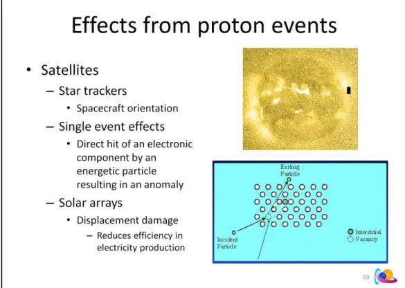
… Satellites can be oriented by the use of star sensors (and Sun sensors). For example, scientific satellites in orbit around Earth may need to know the Sun direction for use in interpreting data from on-board scientific instruments. Star sensors are used for scientific astronomical satellites, as well as for national security and other civil satellite purposes, such as communications. Charged particle radiation can produce false signals in the optical sensors, thus confusing the electronics—with resulting confusion of the orientation. In regions of intense radiation, such as during intervals of enhanced Van Allen belt radiation within Earth’s magnetosphere, and during large solar particle events outside the magnetosphere, star and Sun sensors can be severely compromised.

A good example of a proton storm induced orientation problem was on 1 September 2014 with ST-B. See the news item at http://www.stce.be/news/266/welcome.html as well as https://sohowww.nascom.nasa.gov/pickoftheweek/old/05sep2014/ Galvan et al. (2014): Satellite Anomalies

http://www.rand.org/content/dam/rand/pubs/research_reports/RR500/RR560/RAND_RR560.pdf

Single Event Effects (SEEs) - SEEs are anomalies caused not by a gradual buildup of charge over time as with surface or internal charging, but by the impact of a single high-energy charged particle into sensitive electronic components of a satellite subsystem, this single event causing ionization and an anomaly. They typically occur because of high-energy (> 2 MeV) protons and electrons striking memory devices in the spacecraft’s electronics systems, causing the spacecraft (or a subsystem) to halt operations, either temporarily or permanently (e.g., Speich and Poppe, 2000).

… Susceptibility to SEEs depends strongly on system design, and the risk is higher for satellites spending time in the Van Allen radiation belts or at GEO where there is a higher fluence of galactic cosmic rays and high-energy protons from Solar Proton Events (e.g., Mikaelian, 2001; Wertz and Larson, 1999;).

Figure taken from Valtonen (2004): Space Weather: Effects on Space Technology http://slideplayer.com/slide/3603908/ (slide 33)

Curdt et al. (2015): Solar and Galactic Cosmic Rays Observed by SOHO http://adsabs.harvard.edu/abs/2015CEAB...39..109C (Figure 5)

Fig. 5 shows the degradation of the solar array efficiency from Dec 1995 until Feb 2013. The total loss was ~22.5% during that time (and has reached 24% at the end of 2014). … a phase of several stepwise decrements that can be associated to SEP events during the maximum of cycle 23 around 2001. Here, individual proton events start to dominate the scene ...

(60)

Figure taken from http://wwwgro.sr.unh.edu/neutron_monitors/shower.gif

Perrone et al. (2004): Polar cap absorption events of November 2001 at Terra Nova Bay, Antarctica http://adsabs.harvard.edu/abs/2004AnGeo..22.1633P

The occurrence of SPE during minimum solar activity is very low, while in active Sun years, especially during the falling and rising phase of the solar cycle,

the SPEs may average one per month. It is well recognised that these solar particles have prompt and nearly complete access to the polar atmosphere via magnetic field lines interconnected between the interplanetary medium and the terrestrial field (van Allen et al., 1971). Consequently, they cause excess ionisation in the ionosphere, particularly concentrated in the polar cap, which, in turn, leads to an increase in the absorption of HF radio waves, termed polar cap absorption (PCA).

The ionisation occurs at various depths which depends on the incident particle energies, so that the ionisation in the D-region during PCA events is due mainly to protons with energy in the range of 1 to 100MeV that

corresponds to an altitude between 30–80 km (Ranta et al., 1993; Sellers et al., 1977; Collis and Rietveld, 1990; Reid, 1974). Particles with even greater energies (>500 MeV) are recorded on the ground by a cosmic-ray detector; these events are called Ground Level Enhancement (GLE) (Davies, 1990).

Thakur et al. (2014): Ground Level Enhancement in the 2014 January 6 Solar Energetic Particle Event http://adsabs.harvard.edu/abs/2014ApJ...790L..13T

Solar energetic particle (SEP) events, where particles accelerated to GeV energies are subsequently detected on the ground as a result of the air-shower process, are known as ground level enhancements (GLEs). With a typical detection rate of a dozen GLEs per cycle, an average of 16.3% SEP events were GLEs in cycles 19–23 (Cliver et al. 1982; Cliver 2006; Shea & Smart 2008; Mewaldt et al. 2012; Nitta et al. 2012; Gopalswamy et al. 2012a). In cycle 24, this fraction is much smaller (6.4%) with 2 GLEs out of 31 large SEP events (Gopalswamy et al. 2014). This is also much smaller than the ratio of 18% obtained when the first five years of cycle 23 are considered. GLEs are typically associated with intense flares (median soft X-ray intensity ∼X3.8) and fast coronal mass ejections (CMEs; average CME speed ∼2000 km s−1; see Gopalswamy et al. 2012a).

(61)

Links

Radiation dose: http://www.radiologyinfo.org/en/info.cfm?pg=safety-xray (normal yearly background: 3 mSv; chest x-ray: 0.1 mSv)

ESA career limit: http://adsabs.harvard.edu/abs/2014JSWSC...4A..20J Flight Safety: https://flightsafety.org/asw-article/flare-ups/

ESA SSA: http://swe.ssa.esa.int/nso_air

NASA: https://srag.jsc.nasa.gov/Publications/TM104782/techmemo.htm

EPCARD: http://www.helmholtz-muenchen.de/en/epcard-portal/information/determining-radiation-exposure-of-airline-staff/index.html

Space Weather index dor radiation at aviation altitudes: http://adsabs.harvard.edu/abs/2014JSWSC...4A..13M Pregnancy foetus: http://publicsafety.tufts.edu/ehs/radiation-safety/more-information/pregnancy-and-radiation/ (5mSv over entire pregnancy, 0.5 mSv/month)

From https://www.translatorscafe.com/unit-converter/en/radiation-absorbed-dose/18-25/milligray-millisievert/ Radiation. Absorbed Dose

The absorbed dose characterized the amount of damage done to the matter (especially living tissues) by ionizing radiation. The absorbed dose is more closely related to the amount of energy deposited.

The SI unit of absorbed dose is the gray (Gy), which is equal to J/kg. 1 gray represents the amount of radiation required to deposit 1 joule of energy in 1 kilogram of any kind of matter. The sievert (Sv) is the International System of Units (SI) derived unit of equivalent radiation dose, effective dose, and committed dose. One sievert is the amount of radiation necessary to produce the same effect on living tissue as one gray of high-penetration x-rays. Quantities that are measured in sieverts are designed to represent the biological effects of ionizing radiation.

1 mSv = 1 mGy = 100 mRem = 100 mRad

https://www.translatorscafe.com/unit-converter/en/radiation-absorbed-dose/18-25/milligray-millisievert/ There’s also an excellent discussion of the topic at https://hps.org/publicinformation/ate/q10540.html

(62)

(63)

Topright picture

Kataoka et al. (2006): Flux enhancement of radiation belt electrons during geomagnetic storms driven by coronal mass ejections and co-rotating interaction regions

http://adsabs.harvard.edu/abs/2006SpWea...4.9004K Topleft picture

Kilpua et al.: Unraveling the drivers of the storm time radiation belt response http://adsabs.harvard.edu/abs/2015GeoRL..42.3076K

SIR/CIR

Jian et al. (2006): Properties of Stream Interactions at One AU During 1995 2004 http://adsabs.harvard.edu/abs/2006SoPh..239..337J

Jian et al. (2010): http://www-ssg.sr.unh.edu/mag/JointMeet/Jian_SIRs.pdf More info on (C)IR and SBC in this STCE News item: SBC or CIR?

More info on associated shocks in this news item: Shocking news http://www.stce.be/news/229/welcome.html

(64)

(65)

Definition from NASA:

https://www.nasa.gov/mission_pages/sunearth/science/magnetosphere2.html Animation from https://commons.wikimedia.org/wiki/File:Animati3.gif

Created by Dr Tsyganenko (NASA)

More info and animations at http://geo.phys.spbu.ru/~tsyganenko/modeling.html

Note that planets without a (strong) intrinsic magnetic field have an “induced magnetosphere”, for which the above defintion obviously is not applicable. However, this is also not the focus of this lecture, which will consider the earth environment only.

“Induced magnetospheres” by Luhmann et al. (2004)

https://www.sciencedirect.com/science/article/pii/S0273117704000158

Induced magnetospheres occur around planetary bodies that are electrically conducting or have substantial ionospheres, and are exposed to a time-varying external magnetic field. They can also occur where a flowing plasma encounters a mass-loading region in which ions are added to the flow. In this introduction to the subject we examine induced magnetospheres of the former type. The solar wind interaction with Venus is used to illustrate the induced magnetosphere that results from the solar wind interaction with an ionosphere.

(66)

See http://sci.esa.int/cluster/51744-magnetic-reconnection-in-earth-s-magnetosphere/ for another animation

A full description of the evolution of a geomagnetic (sub)storm can be found in the SIDC SWx Forecast Guide: http://www.sidc.be/PRODEX_SIDEx/docs/Space_Weather_Forecasting_Guide_latest.pdf

(67)

Figure from Stankov et al. (2010): Local Operational Geomagnetic Index K Calculation (K-LOGIC) from digital ground-based magnetic measurements

(68)

On the K and Kp index: SWPC: https://www.swpc.noaa.gov/sites/default/files/images/u2/TheK-index.pdf Potsdam: https://www.gfz-potsdam.de/en/kp-index/

The reported values, be they updated every hour or every 3 hours, always cover the recordings of the last 3 hours. E.g. the 10UT value reported by Dourbes covers the interval 07-10UT.

The estimated Kp values are the ones that can be found at NOAA/SWPC: https://www.swpc.noaa.gov/products/planetary-k-index

The final Kp values are determined by GFZ Potsdam and can be downloaded at Kyoto WDC: http://wdc.kugi.kyoto-u.ac.jp/kp/index.html

The maps for auroral visibility can be found at https://www.swpc.noaa.gov/content/tips-viewing-aurora Left figure taken from HAO/UCAR SW103 Lecture 4: Geomagnetic indices and space weather models. https://www2.hao.ucar.edu/sites/default/files/users/whawkins/SW102_4_Indices.pdf

The nomenclature is the one mentioned in NOAA/SWPC ’ User guide. https://www.swpc.noaa.gov/sites/default/files/images/u2/Usr_guide.pdf

The 13 observatories for Kp are (currently operational: https://www.gfz-potsdam.de/en/kp-index/):

Sitka, Alaska, USA; Meanook, Canada; Ottawa, Canada; Fredericksburg, Virginia, USA; Hartland, UK; Wingst, Germany; Niemegk, Germany; Canberra, Australia; Brorfelde, Denmark; Eyerewell, New Zealand; Uppsala, Sweden; Eskdalemuir, UK; Lerwick, UK.

All these stations have geomagnetic latitudes between 35° and 60°. This zone is called the subauroral zone.

The main purpose of the standardized index Ks is to provide a basis for the global geomagnetic index Kp which is the average of a number of "Kp stations", originally 11. The Ks data for the two stations Brorfelde and Lovö/Uppsala, as well as for Eyerewell and Canberra, are combined so that their average enters into the final calculation, the divisor thus remaining 11. The Estimated 3-hour Planetary Kp-index is derived at the NOAA Space Weather Prediction Center using data from the following ground-based magnetometers: Sitka, Alaska; Meanook, Canada; Ottawa, Canada; Fredericksburg, Virginia; Hartland, UK; Wingst, Germany; Niemegk, Germany; and Canberra, Australia.

(69)

The « G » stands for Geomagnetic storms. Note it starts only from Kp =5 or higher. More at http://www.stce.be/news/366/welcome.html

(70)

More on the NOAA-scales at at http://www.stce.be/news/366/welcome.html

Each graph shows the yearly accumulation of the events, with the yearly International Sunspot Number (SILSO) superposed on it as the gray dashed line.

The plot of the geomagnetic storm days bears much less resemblance with the evolution of the sunspot number than in the previous two charts. This is because minor to strong geomagnetic disturbances can also be caused by the high speed solar wind streams (HSS) from coronal holes, hence distorting the familiar outlook of the sunspot cycle. Nonetheless, even then it is very clear that SC24 has been quite disappointing when it comes to the number and intensity of geomagnetic storms, with no extreme storms (G5) so far and precious few severe events (G4). Worse, the numbers even get depressingly low when one compares to other years such as e.g. the 120 storming days in 2003. Interestingly, the number of geomagnetic storm days is peaking in 2015-2016, so after the SC24 maximum in 2014. This is particularly due to the HSS from numerous coronal holes, and is a well-known aspect of this stage of a solar cycle.

More on SC24 geomagnetic performance at http://www.stce.be/news/243/welcome.html A quick analysis of the final Kp indices as archived at the Kyoto World Data Centre (WDC) for geomagnetism reveals that the current solar cycle (SC24) is really underperforming so far. Not only has there not been any day with extreme geomagnetic storming, SC24 also has a lot more "quiet" days compared to the average of the previous 7 solar cycles (SC17-23). Of course, most of those cycles had already passed their maximum for 1-2 years, whereas SC24 is peaking only now and at a much lower solar activity level.

(71)

From GFZ/Potsdam: https://www.gfz-potsdam.de/en/kp-index/

The three-hour index ap and the daily indices Ap, … are directly related to the Kp index. In order to obtain a linear scale from Kp, J. Bartels gave the [above] table to derive a three-hour equivalent range, named ap index. This table is made in such a way that at a station at about dipole latitude 50 degrees, ap may be regarded as the range of the most disturbed of the two horizontal field

components, expressed in the unit of 2nT.

On the aa-index: F. De Meyer (2006): The geomagnetic aa index as precursor of solar activity www.meteo.be/meteo/download/de/520427/pdf/

The availability of magnetic records from two old observatories, Greenwich (51.5° N,0.0° E) and Melbourne (37.8° S,145.0° E), which are almost antipodal, gave the possibility of obtaining a reliable long series if K scalings were made on their records (Mayaud, 1972). The two stations are nearly at the same geomagnetic latitude (one in the northern hemisphere, Greenwich: 50.1°, and one in the southern hemisphere, Melbourne: {48.9°) and about 10 h apart in longitude. The K indices from these two observatories at sub-auroral latitudes were first standardized for the corrected geomagnetic latitude of 50° in order to obtain a value identical with the one that would be obtained at a distance of 19° from the auroral zone. The converted equivalent amplitudes ak of the two stations were then averaged to provide the three-hourly index aa (expressed in units of nanotesla), which aims at monitoring the average intensity of the transient magnetic variations at sub-auroral latitudes. More information on the aa-index also at BGS:

(72)

From GFZ/Potsdam: https://www.gfz-potsdam.de/en/kp-index/

The three-hour index ap and the daily indices Ap, … are directly related to the Kp index. In order to obtain a linear scale from Kp, J. Bartels gave the [above] table to derive a three-hour equivalent range, named ap index. This table is made in such a way that at a station at about dipole latitude 50 degrees, ap may be regarded as the range of the most disturbed of the two horizontal field

components, expressed in the unit of 2nT.

On the aa-index: F. De Meyer (2006): The geomagnetic aa index as precursor of solar activity www.meteo.be/meteo/download/de/520427/pdf/

The availability of magnetic records from two old observatories, Greenwich (51.5° N,0.0° E) and Melbourne (37.8° S,145.0° E), which are almost antipodal, gave the possibility of obtaining a reliable long series if K scalings were made on their records (Mayaud, 1972). The two stations are nearly at the same geomagnetic latitude (one in the northern hemisphere, Greenwich: 50.1°, and one in the southern hemisphere, Melbourne: {48.9°) and about 10 h apart in longitude. The K indices from these two observatories at sub-auroral latitudes were first standardized for the corrected geomagnetic latitude of 50° in order to obtain a value identical with the one that would be obtained at a distance of 19° from the auroral zone. The converted equivalent amplitudes ak of the two stations were then averaged to provide the three-hourly index aa (expressed in units of nanotesla), which aims at monitoring the average intensity of the transient magnetic variations at sub-auroral latitudes. More information on the aa-index also at BGS:

(73)

Real time monitoring at http://wdc.kugi.kyoto-u.ac.jp/dst_realtime/presentmonth/index.html

Top right figure taken from HAO/UCAR SW103 Lecture 4: Geomagnetic indices and space weather models. https://www2.hao.ucar.edu/sites/default/files/users/whawkins/SW102_4_Indices.pdf

Source: Love J.J., Remick K.J. (2007) Magnetic Indices. In: Gubbins D., Herrero-Bervera E. (eds) Encyclopedia of Geomagnetism and Paleomagnetism. Springer, Dordrecht - https://doi.org/10.1007/978-1-4020-4423-6_178 ;

https://geomag.usgs.gov/downloads/publications/Magnetic_Indices.pdf

One of the most systematic effects seen in ground-based magnetometer data is a general depression of the horizontal magnetic field as recorded at near-equatorial observatories (Moos, 1910). This is often interpreted as an enhancement of a westward magnetospheric equatorial ring current, whose magnetic field at the Earth’s surface partially cancels the predominantly northerly component of the main field. The storm-time disturbance index Dst (Sugiura, 1964) is designed to measure this phenomenon. Dst is one of the most widely used indices in academic research on the magnetosphere, in part because it is well

motivated by a specific physical theory. The calculation of Dst is generally similar to that of AE, but it is more refined, since the magnetic signal of interest is quite a bit smaller. One-min resolution horizontal intensity data from low-latitude observatories are used, and diurnal and secular variation baselines are subtracted. A geometric adjustment is made to the resulting data from each observatory so that they are all normalized to the magnetic equator.

The average, then, is the Dst index. It is worth noting that, unlike the other indices summarized here, Dst is not a range index. The 4 stations are Kakioka (Japan), Hermanus (South Africa), Honolulu (Hawaii, USA), San Juan (USA).

From the SIDC SWx Forecast Guide: http://www.sidc.be/PRODEX_SIDEx/docs/Space_Weather_Forecasting_Guide_latest.pdf The Dst or disturbance storm time index is a measure of geomagnetic activity used to assess the severity of magnetic storms. It is often considered to reflect variations in the intensity of the symmetric part of the ring current that circles Earth at altitudes ranging from about 3 to 8 Earth radii (RE), and is proportional to the total energy in the drifting particles that form the ring current (Wanliss et al. 2006, and references therein). It is calculated as an hourly index from the horizontal magnetic field component (H) at four observatories located close enough to the magnetic equator that they are not strongly influenced by auroral current systems. At the same time, these stations are far enough away from the magnetic equator so that they are not significantly influenced by the equatorial electrojet current that flows in the ionosphere. They are also relatively evenly spaced in longitude … . The convolution of their magnetic variations forms the Dst index, measured in nT, which is thought to provide a reasonable global estimate of the variation of the horizontal field near the equator. So: Dst represents an induced magnetic field caused by the ring current particles, which are plasmasheet particles that are accelerated

(74)