Description of the DEPAC module : Dry deposition modelling with DEPAC_GCN2010

(1)

Report 680180001/2010 M.C. van Zanten et al.

Description of the DEPAC module

Dry deposition modelling with DEPAC_GCN2010

(2)

RIVM Report 680180001/2010

Description of the DEPAC module

Dry deposition modelling with DEPAC_GCN2010

M.C. van Zanten F.J. Sauter

R.J. Wichink Kruit J.A. van Jaarsveld, PBL W.A.J. van Pul

Contact:

Margreet van Zanten

Centrum voor Milieumonitoring margreet.van.zanten@rivm.nl

This investigation has been performed by order and for the account of the ministry of Housing, Spatial Planning and the Environment (VROM), within the framework of project M/680180/10/AG Ammonia

(3)

Parts of this publication may be reproduced, provided acknowledgement is given to the 'National Institute for Public Health and the Environment', along with the title and year of publication.

(4)

Abstract

Description of the DEPAC module

Dry deposition modelling with DEPAC_GCN2010

The process of dry deposition represents the coming down of air components like ammonia on vegetation and soils. Since dry deposition measurements are difficult and expensive, dry deposition estimates are mainly computed through modelling. New insights have led to an update of the description of the dry deposition process. This report presents a detailed description of the revised software-module DEPAC, which simulates the dry deposition process of ammonia.

Dry deposition influences the concentration of a component in the air and is an important source of components for the receiving surface. Thus it is important to estimate the amount of total nitrogen deposited on nature. When too much nitrogen is deposited, biodiversity is harmed since nitrogen-thrifty vegetation is replaced with more common species like grasses and brambles. Dry deposition of

ammonia represents the largest amount of the total nitrogen deposition. Ammonia enters the air predominantly through the process of evaporation from manure in animal stables and when liquid manure is spread over the land.

Earlier versions of the DEPAC module ignored the ammonia concentration in vegetation and soils. The current version assumes that ammonia is present in vegetation, water surfaces and soils. Thus surfaces not only adsorb ammonia but also are able to emit it under certain atmospheric conditions. Further included in the update are an improved description of the light fall in woods and other high vegetation and an improved description of the yearly cycle of the amount of leaf area of plants and trees.

Key words:

(5)

(6)

Rapport in het kort

Beschrijving van de DEPAC module

Droge depositie modellering met DEPAC_GCN2010

Droge depositie is het proces waarbij een stof uit de lucht op de bodem en vegetatie terecht komt. Metingen van het depositieproces zijn omslachtig en duur, daarom wordt de droge depositie met behulp van modellen berekend. Als gevolg van nieuwe inzichten in het droge depositieproces van ammoniak heeft het RIVM de modellering ervan verbeterd. Het rapport beschrijft gedetailleerd de aangepaste softwaremodule (DEPAC) waarmee het droge depositieproces van ammoniak wordt berekend. Droge depositie beïnvloedt de concentratie van de stof in de lucht en is een belangrijke bron van stoffen voor het ontvangende oppervlak. Zo is het van groot belang inzicht te krijgen in de hoeveelheid droge depositie van stikstof op natuurgebieden. Als teveel stikstof deponeert op natuurgebieden, neemt de soortenrijkdom af. Dat komt doordat stikstofminnende planten, zoals grassen en bramen, kwetsbare soorten verdringen. Droge depositie van ammoniak vormt de grootste bijdrage aan de totale

stikstofdepositie. Ammoniak komt voornamelijk in de atmosfeer terecht als mest in stallen verdampt of over het land wordt uitgereden.

De vorige modelversie verwaarloosde de ammoniakconcentratie in de vegetatie en de bodem. De huidige versie veronderstelt dat er ammoniak in de vegetatie, wateroppervlakken en de bodem aanwezig is. De vegetatie neemt daarom niet alleen ammoniak op, maar geeft – onder bepaalde atmosferische omstandigheden – ook ammoniak af aan de lucht. Verder is in de software de

beschrijving van zonlichtinval in bossen verbeterd, evenals het jaarlijkse verloop van het bladoppervlak van de vegetatie.

Trefwoorden:

(7)

(8)

Preface

The deposition module DEPAC (DEPosition of Acidifying Compounds) is available for the calculation of dry deposition fluxes. DEPAC is for instance implemented in the Operational Priority Substance (OPS) model for calculating the large scale deposition maps of the Netherlands (called GDN maps). This technical report describes the entire, updated DEPAC module, version number 3.11. It is mainly aimed at users who want to have a detailed description of all parameterizations in use in DEPAC. This report, however, does not contain an instruction manual.

For those readers who are mainly interested in getting an overview of the updates implemented in DEPAC version 3.11, it would suffice to read Chapter 2. Description of the various exchange pathways of dry deposition can be found in Chapters 3 till 7, while further details of various aspects of the module can be found in the Appendices.

People interested in the effect of the DEPAC update on the GDN maps are referred to Velders et al., 2010.

(9)

(10)

Summary

For many years, a difference of roughly 25% existed between the ammonia concentrations as measured by the Dutch Monitoring Network and the ammonia concentrations as modelled by the Operational Priority Substance (OPS) model (Van Jaarsveld, 2004). In Van Pul et al. (2008) the combination of factors leading to this so called ‘ammonia gap’ are described. Too high dry deposition fluxes of ammonia in OPS were one of them, leading to an underestimation of the concentration of ammonia in the air. In this report the subsequent update of the dry deposition processes is described.

Focus of the update has been on the parameterizations specifically in use for ammonia, although changes have been made that affect other components as well (if the updated version is applied to those components). The major changes are:

1. For ammonia, so called compensation points have been implemented for the stomatal, external leaf surface and soil exchange pathway.

2. The external leaf surface resistance of ammonia has been replaced by the one of Sutton and Fowler (1993), which should be used in combination with the external leaf surface

compensation point.

3. The stomatal resistance scheme of Wesely (1989) has been replaced by the more process oriented stomatal resistance scheme of Emberson (2000a, b). This change has an impact on all components.

4. The leaf area index has been taken from Emberson (2000a). This change has an impact on all components.

5. The in-canopy resistance for land use classes grass and other is set to missing. This change has an impact on all components.

6. Some changes have been made in order to make the former DEPAC versions used for LOTOS-EUROS and OPS consistent. These changes have an impact on NO and SO2.

(13)

(14)

1 Introduction

For many years, a systematic difference of roughly 25% existed between the ammonia concentrations as measured by the Dutch Monitoring Network (LML) and the ammonia concentrations as modelled by the Operational Priority Substance (OPS) model (Van Jaarsveld, 2004). In Van Pul et al. (2008) the combination of factors leading to this so called ‘ammonia gap’ are described. Too high dry deposition fluxes of ammonia in OPS were one of them, leading to an underestimation of the concentration of ammonia in the air. As a consequence, the module estimating the dry deposition flux has been revised. During the revision most attention has been paid to an update of the dry deposition of ammonia. This report describes the entire, updated DEPAC (DEPosition of Acidifying Compounds) module, version number 3.11. This report, however, does not contain an instruction manual of the module, e.g. a detailed list of recommended parameter settings etc. Furthermore, no results of sensitivity tests or validation results are presented. The report contains solely a detailed description of all

parameterizations in use in DEPAC. A concise description of an older DEPAC (version 3.3) currently still in use, is given in Appendix A. The original version of DEPAC has been documented in Erisman et al. (1994). DEPAC is implemented in OPS (Van Jaarsveld, 2004), but also in LOTOS-EUROS (Schaap, 2008).

For the calculations of the large scale concentration maps (called GCN-maps) of 2009 (released March 2010) two versions of DEPAC are in use for the various gaseous components. The updated version (version number 3.11) is applied for NH3 and the older version (version number 3.3) is applied

for the other components: HNO3, NO, NO2, O3, SO2. The shell around these two DEPAC versions is

named DEPAC_GCN2010. Implementation of the new version for the other components besides ammonia, is foreseen after more thorough testing of the update for those components. Revision of the code specific for those components might be necessary.

Due to the update of the DEPAC module, the systematic overestimation of the dry deposition velocity for ammonia above land use class grass has been reduced. This has contributed substantially towards the closure of the ammonia gap (Velders et al., 2010). Proper validation of the updated DEPAC module is hampered by the lack of dry deposition measurements. Up till now most deposition measurements are used to construct the deposition parameterization itself and as such cannot be used for validation. The uncertainty in the local dry deposition velocity is estimated to be a factor two. This is an educated guess and further research is a prerequisite to specify the uncertainty more accurately. Both a validation study as well as an uncertainty analysis is planned for the near future.

(15)

(16)

2 Overview of the DEPAC update.

Dry deposition is parameterized using the well-known resistance approach, where the deposition flux is the result of a concentration difference between atmosphere and earth surface and the resistance between them. The current DEPAC versions compute only the so called canopy resistance, Rc. The aerodynamic resistance for the turbulent layer, Ra, and the boundary-layer resistance, Rb, are calculated outside DEPAC.

Focus of the update has been on the parameterizations specifically in use for ammonia, although changes have been made that affect all components (in the case that v.3.11 is applied to those components). The major changes, either in code size or in impact, in v.3.11 compared to v.3.3 are:

1. For ammonia, so called compensation points have been implemented for the stomatal, external leaf surface and soil exchange pathway (Wichink Kruit et al., 2010).

2. The external leaf surface resistance of ammonia has been replaced by the one of Sutton and Fowler (1993), which should be used in combination with the external leaf surface

compensation point (Wichink Kruit et al., 2010).

3. The stomatal resistance scheme of Wesely (1989) has been replaced by the more process oriented stomatal resistance scheme of Emberson (2000a, b). This change has an impact on all components.

4. The leaf area index has been taken from Emberson (2000a). This change has an impact on all components.

5. The in-canopy resistance for land use classes grass and other is set to missing. This change has an impact on all components.

6. Some changes have been made in order to make the former DEPAC versions used for LOTOS-EUROS and OPS consistent. These changes have an impact on NO and SO2.

The above changes will be described in more detail below. Full details can be found in the rest of the report.

1. Compensation points. Up till now, only deposition fluxes were calculated in DEPAC and no

emission fluxes were allowed. In the current version, the flux is allowed to be bidirectional by

including compensation points in the stomatal, external leaf surface and the soil exchange pathway (see Figure 1 for a schematic picture). Compensation points are in use for all land use classes. (Chapter 3). Both the stomatal and the external leaf surface compensation point depend on temperature and ammonia concentration in the air. However, the stomatal compensation point represents the ammonia present in the vegetation and thus is tied to a fairly long timescale (e.g. the local yearly mean). Since ammonium concentrations in water layers present on leaves have a short memory, the external leaf compensation point is linked to the actual ammonia concentration in the air. Both compensation point parameterizations have been derived based on three years of measurements of ammonia fluxes over a grassland canopy (Wichink Kruit et al., 2010). (Chapter 6 and chapter 4).

For the soil compensation point not enough information is known to implement a parameterization, so this variable is currently set to zero. Only for land use class water a simple water compensation point parameterization with a dependency on water temperature is derived, based on five years of

measurements at several locations in fresh water bodies and the North Sea. This parameterization is in first instance valid for Dutch locations only. (Chapter 5).

(17)

2. External leaf surface resistance. The external leaf surface resistance for ammonia is based on Sutton

and Fowler (1993) and is dependent on ambient relative humidity only. This parameterization is representative for clean air; the influence of pollution is accounted for in the external leaf surface compensation point value. The Sutton and Fowler parameterization should always be used in combination with a compensation point, since neglecting this compensation point would lead to an overestimation of ammonia deposition through the external leaf exchange pathway. (Chapter 4).

3. Stomatal resistance. The stomatal resistance scheme of Emberson (2000a,b) has been implemented;

this scheme is also in use in the European Modelling and Evaluation Programme (EMEP) model. In this scheme, several factors are used to scale a minimal resistance value. One factor takes into account the availability of light; in this factor a difference is made between direct and diffuse sunlight on sunlit and shaded leaves. Other environmental factors accounted for are temperature and water vapour deficit. The phenological factor of the Emberson scheme is not implemented, since this factor is negligible for the land use classes used in DEPAC. The effect of a deficit of soil moisture is not implemented either. (Chapter 6).

4. Leaf area index. The monthly changing Leaf Area Index (LAI) values have been replaced by ones

with a dependency on the day of year to ensure a better representation of the growing season (Emberson, 2000a). A latitude dependent effect on the length of the growing season is now also included. The LAI is used in the upscaling of the leaf stomatal resistance to a stomatal resistance valid for the whole canopy. A Surface Area Index (SAI) has been introduced for the upscaling of the external leaf resistance from leaf to canopy scale. SAI is commonly larger than LAI due to the presence of branches and stems. (Appendix B.

5. In-canopy resistance. The in-canopy resistance for land use class grass (and other since this class is

modelled identically to grass) is set to missing instead of zero. This shuts off the soil exchange path completely. (Chapter 5).

6. Changes for consistency. Before this DEPAC update, a few differences existed between the OPS

DEPAC version and the LOTOS-EUROS version with regard to SO2 and NO. In version 3.11 these

(18)

3 Dry deposition using a compensation point model

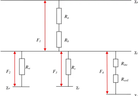
In the dry deposition module DEPAC, dry deposition is parameterized using the well-known resistance approach, where the deposition flux is the result of a concentration difference between atmosphere and earth surface and the resistance between them. Several pathways exist for the deposition flux, each with its own resistance and concentration. In DEPAC three pathways are taken into account:

• through the stomata (subscript s);

• through the external leaf surface (water layer or cuticular waxes, subscript w); and • through the soil (subscript soil).

The concentration in the stomata, at the external leaf surface or at the soil surface is for historic reasons called a compensation point.

A schematic representation of concentrations χ, resistances R and fluxes F is given in Figure 1.

Figure 1. Schematic representation of resistance approach with compensation points.

χw F4 F3 F2 F1 Ra Rb Rs χa χs χc Rw Rinc Rsoil χsoil

(19)

name of parameter

unit name in DEPAC

explanation

χa µg/m3 catm concentration in air

χc µg/m3 concentration at canopy top

χw µg/m3 cw concentration at external leaf surface

χsoil µg/m3 csoil concentration at soil surface

χs µg/m3 cstom concentration in stomata

Ra s/m ra aerodynamic resistance

Rb s/m rb quasi-laminar layer resistance

Rw s/m rw external leaf surface or water layer resistance, also called

cuticular resistance

Rs s/m rstom stomatal resistance

Rinc s/m rinc in canopy resistance

Rsoil s/m rsoil soil resistance

Rsoil,eff s/m rsoil_eff effective soil resistance = Rinc + Rsoil

Rc s/m rc_tot canopy resistance

In the text below, we distinguish between upper case and lower case characters:

r: leaf resistance;

R: canopy averaged resistance;

g: leaf conductance = 1/r;

G: canopy averaged conductance G = 1/R.

For the external leaf conductance, G = SAI g, with SAI = surface area index (i.e. the area of leaves, branches and stems per unit area of ground surface).

For the stomatal conductance, G = LAI g, with LAI = leaf area index (i.e. the area of leaves per unit area of ground surface).

More information on LAI and SAI can be found in Appendix B. The fluxes F over the different pathways in Figure 1 are:

(

)

(

)

s s c eff soil soil c w w c b a c a

R

F

R

F

R

F

R

F

(

)

,

₄

(

)

, 3 2 1

χ

₌

₋

−

₌

₋

−

₌

₋

−

+

−

=

. (1)

We define the canopy resistance

1 ,

1

−













+

=

s eff soil w c

R

, (2)

the exchange velocity

c b a e

R

V

+

=

1

(3)

and the total compensation point













+

=

s s c soil eff soil c w w c tot

R

_χ

χ

, . (4)

(20)

(

)

.

1

V

e a tot

F

=

−

χ

−

χ

. (5)

The mass balance in a layer with height H is:

)

(

1 e a tot a

_F

_V

t

H

χ

=

−

⋅

χ

−

χ

∂

. (6)

If we assume a constant value of

χ

_tot(large reservoir) on a time interval

[

t

,

t

+

∆

t

]

, we get as solution:

(

)

(

)

exp(

t

)

H

V

t

e tot a tot a

+

∆

=

χ

+

χ

−

χ

⋅

−

⋅

∆

χ

. (7)

An alternative method (Asman, 1994), that puts the compensation point into an effective resistance, is presented in Appendix G.

In the following sections, we will describe the parameterizations of the different resistances that contribute tot the canopy resistance Rc for dry deposition of NH3. Parameterizations of Ra and Rb can be

found in Van Jaarsveld (2004).

Resistance parameterizations are different for different land use types. In DEPAC the following land use types are used:

1 = grass 2 = arable land 3 = permanent crops 4 = coniferous forest 5 = deciduous forest 6 = water 7 = urban 8 = other 9 = desert

In the text we will use ‘forest’ for both coniferous and deciduous forest. For more information on land use classes, see Appendix B.

(21)

(22)

4 External leaf surface exchange

In DEPAC, we use the following parameterization for the canopy averaged external leaf surface resistance:













−

⋅

=

β

α

RH

SAI

R

_w Haarweg

exp

100

, (8)

with RH the relative humidity in %, α = 2 s/m, β = 12, SAI = surface area index (i.e. the area of leaves, branches and stems per unit area of ground surface) and SAIHaarweg = surface area index at the Haarweg measuring site (estimated to be 3.5).

The parameterization

_











−

⋅

β

α

exp

100 RH

,

represents the minimum external leaf surface resistance, Rw,min (Sutton and Fowler, 1993) that only accounts for the relative humidity response and is valid for clean conditions (this assumption is supported by the findings of Milford et al., 2001b). The higher Rw values at 100% relative humidity found in literature (Nemitz et al., 2001) reflect different air pollution climates, as well as potential variation in NH3 supply from the canopy itself, which will be accounted for in

χ

w.

The scaling factor

SAI

_Haarweg

,

takes into account that for a different vegetation type, the surface area index of the vegetation may be different from that of the measuring site, for which the parameterization of

χ

w was derived.

At the external leaf surface water interface, the gaseous NH3 concentration,

χ

w, may be considered as

being in equilibrium with the dissolved NH4 +

concentration. The theoretical relationship between the gaseous ammonia concentration, leaf surface temperature (Ts), ammonium concentration and pH, can be derived from the temperature response of the Henry equilibrium for ammonia, NH3(g) ↔ NH3(aq),

and the ammonium-ammonia dissociation equilibrium, NH3(aq) + H +

(aq) ↔ NH4 +

(aq). The theoretical atmospheric NH3 concentration at the leaf surface water interface,

χ

w, can be calculated analogous to

the stomatal compensation point (following the formulation of Nemitz et al., 2001, and Wichink Kruit et al., 2007): w s s w

T



_

⋅

Γ









+

⋅

−

+

⋅

=

15 .

273

10

04 .

1 exp

15 .

273

10

75 .

2

15 4

χ

(9)

where

χ

w is the gaseous NH3 concentration at the external leaf surface (µg m -3

), Ts is the leaf surface temperature (°C) and Γw is the dimensionless molar ratio between the NH4

+

and H+ concentrations in the external leaf surface water.

An empirical relation for Γw is derived for grassland by Wichink Kruit et al. (2010):

(

0 .

11 )

850 exp

10

84 .

1 ⋅

3

⋅

_,₄

⋅

−

⋅

−

=

Γ

_w

χ

_a _m

T

_s (10)

(23)

where

χ

a,4m is the actual atmospheric ammonia concentration at 4 m height in μg m-3 and Ts is the leaf surface temperature in °C.

The functional behaviour of

χ

w

and

Γ

wis shown in Appendix F. As can be seen from this appendix,

the external leaf compensation point is always smaller than the atmospheric concentration and thus emissions from plant to atmosphere will not take place. Models that do not have the actual atmospheric concentration available may use a long-term averaged concentration. In this case, emission might occur in certain circumstances.

Here, we assume that the parameterization for Γw is also valid for other vegetation types, as it is not supposed to be a plant property. Or formulated alternatively, we expect concentration and temperature dependencies to be more important than the dependency on vegetation type.

(24)

5 Soil exchange

The soil resistance (s/m) is given as follows (Erisman et al 1994, note that here 0 is interpreted as 'negligible' and the corresponding resistance is set to 10 s/m):

Frozen soil :

R

_soil= 1000 s m-1.

non-frozen soil, dry :

R

_soil= 10 s m-1 , water. (11)

R

_soil= 100 s m-1 , all other DEPAC land use classes. non-frozen soil, wet :

R

_soil= 10 s m-1.

The in-canopy resistance is parameterized as (Van Pul and Jacobs, 1994):

*

u

SAI

h

b

R

inc

⋅

=

,

u

*

>

0

, arable land, permanent crops, forest. inc

R

= 1000 s m-1,

u

*

≤

0

, arable land, permanent crops, forest. (12) inc

R

= 0 s m-1, water, urban, desert. inc

R

= ∞ s m-1, grass, other.

with b an empirical constant (14 m-1), h vegetation height (m), SAI surface area index (-) and u* the friction velocity (m/s).

The resistance used for the soil pathway is the effective soil resistance: soil

inc eff

soil

R

,

=

+

. (13)

A soil compensation point

χ

soil is added, analogous to the stomatal compensation point. However, since it is unknown what the best value or best parameterization of

χ

soil should be, its value is currently set to zero. Only for land use class water, a parameterization for

χ

soil (named

χ

water in the text below for clarity) has been added, similar as for

χ

w:

water water water water

T



_

⋅

Γ









+

⋅

−

+

⋅

=

15 .

273

10

04 .

1 exp

15 .

273

10

75 .

2

15 4

χ

(14)

The necessary Γwater and temperature value are based on five recent years of data from the Waterbase data of Rijkswaterstaat. Based on NH4

+

and pH data of seventy stations a representative value for Γwater was derived:

Γwater = 430. (15)

This value is representative for the large water bodies in the Netherlands and the coastal waters, but overestimates

χ

water further away at sea and underestimates

χ

water in polluted rivers and lakes. At 25 of these 70 sites temperature has been measured as well. Based on this data, the following representative yearly cycle of water temperature has been derived:

Twater = 13.05 + 8.3 sin(DOY – 113.5) ºC (16)

with DOY = day of year. More detail about the derivation of the parameterization and figures of measurements and parameterized values of

χ

water at several sites are given in Appendix F.

(25)

(26)

6 Stomatal exchange

In the parameterization of the stomatal resistance we follow Emberson (2000a,b). The parameterization shown here is formulated in terms of conductance G = 1/R. With a lower case g we denote leaf

conductance, upper case G is used for a canopy averaged conductance.

Emberson uses a maximal stomatal conductance (for certain optimal conditions) that is reduced by different correction factors (between 0 and 1):

PAR T vpd phen s s

G

f

G

=

max

⋅

, (17) with s

G

: canopy averaged stomatal conductance (m/s);

max

s

G

: canopy averaged stomatal conductance for optimal conditions (m/s); phen

f

: correction factor for phenology (-); vpd

f

: correction factor for vapour pressure deficit (-); T

f

: correction factor for temperature (-); PAR

f

: correction factor for photoactive radiation (-).

Emberson provides values for the maximal leaf conductance

g

_smax_,reffor a reference gas (ozone), which has to be multiplied by the leaf area index LAI to obtain a canopy conductance:

max , max ,ref sref s

LAI

g

G

=

⋅

. (18)

More information on the leaf area index can be found in Appendix B.

In order to obtain the maximal stomatal conductance for another gas than the reference, we multiply with the ratio of the diffusion coefficients:

max , max ref s ref s

G

D

G

=

, (19)

D : diffusion coefficient of gas (m2/s);

(27)

6.1 Correction for light

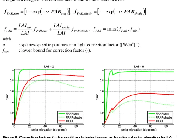
The correction factor fPAR for the influence of the sun's radiation on the stomatal resistance is a weighted average of the corrections for sunlit and shaded leaves:

(

)

[

sun

]

sun

PAR

PAR

f

_,

=

1 −

exp

−

α

,

f

_PAR_,_shade

=

[

1 −

exp

(

−

α

PAR

_shade

)

]

(20) shade PAR shade sun PAR sun PAR

f

LAI

f

LAI

f

=

,

+

, ,

f

PAR

=

max(

f

PAR

,

f

min

)

(21)

with

PAR : photoactive radiation (W/m2);

LAI : leaf area index (m2 leaf /m2 surface);

α : vegetation-specific parameter in light correction factor ([W/m2]-1);

fmin : minimal correction factor (-);

sun : sunlit leaves;

shade : shaded leaves.

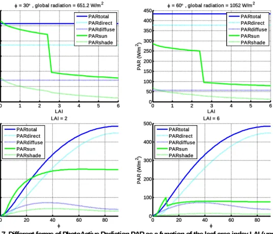
The parameterization of PAR and LAI for sunlit and shaded leaves is described in Appendices C. and D.

6.2 Correction for temperature

The correction factor for temperature fT is taken from Jarvis, 1976. Note that the publication of Jarvis contains an error in the definition of bT ; the correct form is listed below (see also Baldocchi et al.,

1987, p. 97). It is a bell-shaped curve, which indicates that stomata are closed due to low temperatures and to very high temperatures:

T b opt opt T

T

f

_













−













−

=

max max min min _,













−

=

min max

T

b

opt opt T ,

f

T

=

max(

f

T

,

f

min

)

, (22) T : temperature (°C);

Tmin : minimal temperature for open stomata (°C);

Tmax : maximal temperature for open stomata (°C);

bT : factor (-).

(28)

6.3 Correction for vapour pressure deficit

The vapour pressure deficit is parameterized following Monteith (1973):

5 6 4 5 3 4 2 3 2 1

T

a

T

a

T

a

T

a

T

a

T

a

P

sat

=

+

,











 −

⋅

=

100

1 RH

P

vpd

sat , (23)

Psat : saturation vapour pressure (kPa) ;

T : temperature (°C) ;

ai : coefficient (kPa/°Ci ), a1 = 6.113718e-1, a2 = 4.43839e-2, a3 = 1.39817e-3, a4 = 2.9295e-5, a5 = 2.16e-7, a6 = 3.0e-9;

RH : relative humidity (%);

vpd : vapour pressure deficit (kPa).

The correction factor for vapour pressure deficit is

(

)

min max min min min

1 f

vpd

f

_vpd

_

+











−

=

,

f

_vpd

=

max(min(

f

_vpd

,

1 ),

f

_min

)

, (24) with

vpdmin : vapour pressure deficit with minimal conductance (kPa)  fvpd = fmin;

vpdmax : vapour pressure deficit with maximal conductance (kPa)  fvpd = 1.

6.4 Correction for soil water potential

No correction for soil water potential is applied; fswp = 1. We expect that in North-Western Europe, this factor will be of limited influence; in Southern European countries it may be important, but there is not very much information available to compute this correction factor, see Emberson (2000a).

6.5 Correction for phenology

The influence of phenology on stomatal conductance is ignored for now in DEPAC v3.11, since the influence of the functions proposed by Emberson for the land use classes in use in DEPAC is negligible (see appendix B.). When other classes are used (e.g. Mediterranean broadleaf), fphen might be too important to ignore.

(29)

The following table lists the parameters involved in the Emberson parameterization. Values in gray-shaded cells are not used in DEPAC, they are included only for comparison with Simpson (2008).

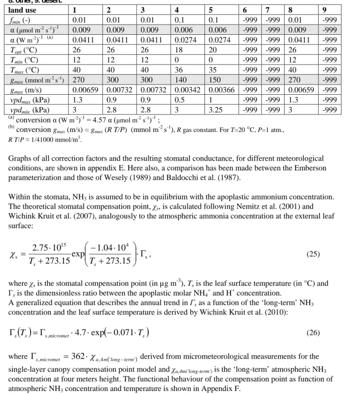
Table 1. parameters for stomatal conductance from Simpson (2008); -999 in case there is no stomatal exchange. 1: grass, 2: arable land, 3: permanent crops, 4: coniferous forest, 5: deciduous forest, 6: water, 7: urban, 8: other, 9: desert. land use 1 2 3 4 5 6 7 8 9 fmin (-) 0.01 0.01 0.01 0.1 0.1 -999 -999 0.01 -999 α (μmol m-2_s-1₎-1 _0.009 _0.009 _0.009 _0.006 _0.006 _{-999 -999 0.009} _-999 α (W m-2₎-1(a) _0.0411 _0.0411 _0.0411 _0.0274 _0.0274 _{-999 -999 0.0411} _-999 Topt (°C) 26 26 26 18 20 -999 -999 26 -999 Tmin (°C) 12 12 12 0 0 -999 -999 12 -999 Tmax (°C) 40 40 40 36 35 -999 -999 40 -999 gmax (mmol m-2 s-1) 270 300 300 140 150 -999 -999 270 -999 gmax (m/s) 0.00659 0.00732 0.00732 0.00342 0.00366 -999 -999 0.00659 -999 vpdmax (kPa) 1.3 0.9 0.9 0.5 1 -999 -999 1.3 -999 vpdmin (kPa) 3 2.8 2.8 3 3.25 -999 -999 3 -999 (a) conversion α (W m-2₎-1_{= 4.57 α (}_{μmol m}-2_s-1₎-1_; (b)

conversion gmax (m/s) = gmax (R T/P) (mmol m-2 s-1), R gas constant. For T=20 °C, P=1 atm.,

R T/P ≈ 1/41000 mmol/m3.

Graphs of all correction factors and the resulting stomatal conductance, for different meteorological conditions, are shown in appendix E. Here also, a comparison has been made between the Emberson parameterization and those of Wesely (1989) and Baldocchi et al. (1987).

Within the stomata, NH3 is assumed to be in equilibrium with the apoplastic ammonium concentration.

The theoretical stomatal compensation point, χs, is calculated following Nemitz et al. (2001) and Wichink Kruit et al. (2007), analogously to the atmospheric ammonia concentration at the external leaf surface: s 4 15 s

15 .

273

10

04 .

1 exp

15 .

273

10

75 .

2 Γ

⋅













+

⋅

−

+

⋅

=

s s

T

χ

, (25)

where χs is the stomatal compensation point (in µg m-3), Ts is the leaf surface temperature (in °C) and Γs is the dimensionless ratio between the apoplastic molar NH4

+

and H+ concentration.

A generalized equation that describes the annual trend in Γs as a function of the ‘long-term’ NH3

concentration and the leaf surface temperature is derived by Wichink Kruit et al. (2010):

( )

s smicromet

(

s

)

s

T

=

Γ

⋅

−

⋅

T

Γ

,

4 .

7 exp

0 .

071

(26)

where

Γ

_s_,_micromet

=

362 ⋅

χ

_a_,₄_m₍_'_long₋_term_'₎ derived from micrometeorological measurements for the single-layer canopy compensation point model and χa,4m('long-term') is the ‘long-term’ atmospheric NH3

concentration at four meters height. The functional behaviour of the compensation point as function of atmospheric NH3 concentration and temperature is shown in Appendix F.

(30)

7 Exchange in case of snow

In case of snow, the above parameterizations are not used; instead there is one overall canopy resistance: c

R

= 500 s m-1 , T < -1 °C ; c

R

= 70 (2-T) s m-1 , -1 °C ≤ T ≤ 1 °C (27) ; c

R

= 70 s m-1 , T > 1 °C.

(31)

(32)

References

Asman, W.A.H. (1994) Emission and deposition of ammonia and ammonium. Nova Acta Leopoldina NF 70, Nr. 288: 263-297.

Baldocchi, D.D., B.B. Hicks and P. Camara (1987) A canopy stomatal resistance model for gaseous deposition to vegetated surfaces. Atmospheric Environment 21: 91-101.

Boer, M. de, J. de Vente, C.A. Mücher, W. Nijenhuis and H.A.M. Thunnissen (2000) An approach towards pan-European land cover classification and change detection, NRSP-2, Report 00-18, Delft. EEA, 2000. Documentation about the Corine landcover 2000 dataset is available from:

http://reports.eea.europa.eu/COR0-landcover.

Emberson, L.D., M.R. Ashmore, D. Simpson, J.-P. Tuovinen and H.M. Cambridge (2000a) Towards a model of ozone deposition and stomatal uptake over Europe. EMEP/MSC-W 6/2000, Norwegian Meteorological Institute, Oslo.

Emberson, L.D., M.R. Ashmore, D. Simpson, J.-P. Tuovinen and H.M. Cambridge (2000b) Modelling stomatal ozone flux across Europe. Water, Air and Soil Pollution 109: 403-413.

Erisman, J.W. and W.A.J. van Pul (1994) Parameterization of surface resistance for the quantification of atmospheric deposition of acidifying pollutants and ozone. Atmospheric Environment 16: 2595-2607.

Jaarsveld, J.A. van (2004) The Operational Priority Substances model. Description and validation of OPS-Pro 4.1. Report 500045001. RIVM, Bilthoven.

Jarvis, P.G. (1976) The interpretation of the variations in leaf water potential and stomata1 conductance found in canopies in the field. Philosophical Transactions of the Royal Society of London, Series B, 273: 593- 610.

Milford, C., K.J. Hargreaves and M.A. Sutton (2001b) Fluxes of NH3 and CO2 over upland moorland

in the vicinity of agricultural land. Journal of Geophysical Research 106: 24169-24181. Monteith, J.L. (1973) Principles of Environmental Physics. Edward Arnold, London.

Nemitz, E., C. Milford C. and M.A. Sutton (2001) A two-layer canopy compensation point model for describing bi-directional biosphere-atmosphere exchange of ammonia. Quarterly Journal of the Royal Meteorological Society 127: 815-833.

Norman, J.M. (1982) Simulation of microclimates. In: Hatfield, J.L. and I.J. Thomason (Eds.), Biometeorology in Integrated Pest Management. Academic Press, New York, pp. 65-99.

Pul, W.A.J. van and A.F.G. Jacobs (1994) The conductance of a maize crop and the underlying soil to ozone under various environmental conditions. Boundary Layer Meteorology 69: 83-99.

(33)

Pul, W.A.J. van, M.M.P. van den Broek, H. Volten, A. van der Meulen, A.J.C. Berkhout, K.W. van der Hoek, R.J. Wichink Kruit, J.F.M. Huijsmans, J.A. van Jaarsveld, B.J. de Haan en R.B.A. Koelemeijer (2008) Het ammoniakgat: onderzoek en duiding. Report 680150002. RIVM, Bilthoven.

Schaap, M., R.M.A. Timmermans, M. Roemer, G.A.C. Boersen, P.J.H. Builtjes, F.J. Sauter, G.J.M. Velders and J.P. Beck (2008) The LOTOS–EUROS model: description, validation and latest developments, Int. J. Environment and Pollution, Vol. 32, No. 2: 270–290.

Simpson, D., H. Fagerli, J.E. Jonson, S. Tsyro, P. Wind and J.P. Tuovinen (2003) Transboundary acidification, eutrophication and ground level ozone in Europe, Part I, EMEP status report.

Simpson, D. (2008) Data from input files for EMEP model: Inputs_DO3SE.csv, Inputs_LandDefs.csv (parameters for land use and stomatal resistance modelling), originally based upon ideas/data in Emberson (2000a); updated to take account of forest-group meeting of Rome, 6-7th Dec. 2007 (L. Emberson, Chair) and of Revisions to Mapping Manual, 2007 (http://www.icpmapping.org/) Sutton, M.A. and D. Fowler D. (1993) A model for inferring bi-directional fluxes of ammonia over plant canopies. Proceedings of the WMO Conference on the Measurement and Modelling of

Atmospheric Composition Changes Including Pollution Transport. WMO/GAW-91, WMO Geneva, pp 179-182.

Sutton, M. A., J.K. Burkhardt, D.Guerin, E. Nemitz and D. Fowler (1998) Development of resistance models to describe measurements of bi-directional ammonia surface-atmosphere exchange,

Atmospheric Environment 32: 473-480.

Velders, G.J.M., J.M.M. Aben, J.A. van Jaarsveld, W.A.J. van Pul, W.J. de Vries, M.C. van Zanten (2010) Grootschalige stikstofdepositie in Nederland. Analyse bronbijdragen op provinciaal niveau. Report 500088007. RIVM, Bilthoven.

Weiss, A. and J.M. Norman (1985) Partitioning solar radiation into direct and diffuse, visible and near-infrared components. Agric. Forest Meteorol. 34: 205-213.

Wesely, M.L. (1989) Parameterization of surface resistances to gaseous dry deposition in regional scale numerical models. Atmospheric Environment 23: 1293-1304.

Wichink Kruit, R.J., W.A.J. van Pul, R.P. Otjes, P. Hofschreuder, A.F.G. Jacobs and A.A.M. Holtslag (2007) Ammonia fluxes and derived canopy compensation points over non-fertilized agricultural grassland in The Netherlands using the new gradient ammonia - high accuracy - monitor (GRAHAM). Atmospheric Environment 41: 1275-1287.

Wichink Kruit, R.J., W.AJ. van Pul, F.J. Sauter, M. van den Broek, E. Nemitz, M.A. Sutton, M. Krol and A.A.M. Holtslag (2010) Modeling the surface-atmosphere exchange of ammonia. Atmospheric Environment, Vol. 44, 7: 877-1004.

Zhang L., M.D. Moran and J.R. Brook (2001) A comparison of models to estimate in-canopy photosynthetically active radiation and their influence on canopy stomatal resistance Atmospheric Environment 35: 4463–4470.

(34)

Appendix A. Description of DEPAC v3.3

Version 3.3 of DEPAC contains the original parameterizations for calculating the canopy resistance Rc as described in Erisman et al. (1994) and Appendix I in Van Jaarsveld (2004). Compared to the original DEPAC, the code of version 3.3 has been restructured and better documented. The text below is an integral copy of the relevant sections of this appendix, for the full text we refer the reader to Van Jaarsveld (2004). A few differences exist between the description and the actual code; those are added in the text.

The canopy resistance

The canopy resistance

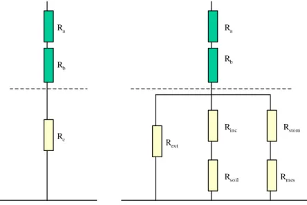
R

_c may be considered as the result of a number of sub-resistances representing different processes in and at the canopy. The general model with the canopy resistance split up in sub-resistances is given in Figure 2.

Figure 2. Resistance model with sub-resistances for the canopy resistance Rc.

In this model Rstom and Rmes represent the stomatal and mesophyll resistances of leaves respectively. Rinc and Rsoil are resistances representing in-canopy vertical transport to the soil, which bypasses leaves and branches. Rext is an external resistance, which represents transport via leaf and stem surfaces, especially when these surfaces are wet. The (effective) canopy resistance Rc can be calculated as:

ext soil inc mes stom c

R

1

1 +

+

=

A.1. Rsoil R_inc Rext R_stom Rmes R_b Ra Ra R_b Rc

Resistance model for acidifying compounds Basic resistance model

(35)

The DEPAC module contains parameters for each of the resistances given in Figure 2 for various land-use types and for each of the gaseous components. Furthermore, a seasonal distinction is made in the values of some of the resistances. In a number of cases the general resistance model reduces to its most basic form, that is, when detailed information is lacking (e.g. for HNO3) or when the surface is

non-vegetative such as for bare soil, water surfaces, buildings or when there is a snow-cover. In these cases only Rsoil determines the effective canopy resistance, because Rext and Rstom are set to (near) infinity. Water surface:

R

_c

=

R

_soil

=

R

_water;

Bare soil:

R

_c

=

R

_soil;

Snow cover:

R

_c

=

R

_soil

=

R

_snow;

HNO3

R

c

=

R

soil.

Stomatal resistance

stom

R

is calculated according to Wesely (1989):

)

40 (

400

1 .

0

200

1

2 , 2 s s i O H stom

T

Q

R

−

⋅

























+

⋅

=

A.2. and x O H O H stom x stom

D

R

2 2 , ,

=

⋅

A.3.

where Q is the global radiation in

W

m

-2,

T

_s the surface temperature in

°

C

,

D

_H_O

2 the molecular

heat diffusivity of water vapour and

D

_xthe molecular heat diffusivity of the substance, both in m2 s-1. i

R

values are given in Table 2. Values of -999 in this and further tables indicate that the resistance is near infinity and plays no role under the given conditions.

Table 2. Ri values at different conditions according to Wesely (1989) (in s m-1).

Season Grass land Arable land Permanent crops Coniferous forest Deciduous forest

Water Urban Other grassy area Desert Summer 60 60 60 130 70 -999 -999 60 -999 Autumn -999 -999 -999 250 -999 -999 -999 -999 -999 Winter -999 -999 -999 400 -999 -999 -999 -999 -999 Spring 120 120 120 250 140 -999 -999 120 -999 Mesophyll resistance

The mesophyll resistance

R

_m is set at 0

s

m

-1 for all circumstances because there are indications that it is low for substances as SO2, O3 and NH3 and because of lack of relevant data to justify other values

(36)

In-canopy resistance

inc

R

represents the resistance against turbulent transport within the canopy and is calculated according to Van Pul and Jacobs (1994):

*

u

h

LAI

b

R

_inc

=

⋅

A.4.

+ where b is an empirical constant (14 m-1

), h the height of the vegetation in m (1 m for arable land and 20 m for forests) and LAI the Leaf Area Index (dimensionless). The authors themselves qualify Equation A.4. as still preliminary. DEPAC uses LAI as a function of the time of the year according to Table 3. The calculation of Rinc according to Eq. A.4. is only carried out for arable land and forest. For all other land-use classes Rinc is set at 0. Note, in current code version 3.3 is Rinc not only calculated for arable land and forests, but for permanent crops as well.

Table 3. Leaf Area Indexes for some land-use classes.

Grass Arable land Perm. Crops* Conif. forest Decid. Forest

Water Urban Other grassy area$

Desert

May and October 6 1.25 1.25 5 1.25 N/A N/A 6 N/A

June and September 6 2.5 2.5 5 2.5 N/A N/A 6 N/A

July and August 6 5 5 5 5 N/A N/A 6 N/A

November - April 6 0.5 0.5 5 0.5 N/A N/A 6 N/A

* The LAI of permanent crops is taken equal to the LAI of arable land. In the original Table in Van Jaarsveld (2004) LAI values were given as N/A.

$ The LAI of other grassy area is taken equal to the LAI of grass. In the original Table in Van Jaarveld (2004) LAI values were given as N/A.

Soil resistance

DEPAC uses

R

_soil values as given in Table 4. The general effect is that wet surfaces enhance the uptake of (soluble) gases. If the soil is frozen and/or covered with snow then the uptake is much less.

Table 4. Soil resistances in s m-1_{for various substances. The values apply to all land-use types including urban}

areas.

Rsoil_wet Rsoil_dry R_soil_frozen& Rwater Rsnow

SO2 10 1000 500 10 70(2-T) $ NO2 2000 1000 2000 2000 2000 NO -999 -999** -999 2000 2000 HNO3 10 10 10 10 50 # NH3 10 100** 1000 10 70(2-T)$ & if T < -1oC. #

only if T < -5 oC, otherwise Rsnow = 10 s m-1. $

minimal value = 70; if T< -10C, Rsnow = 500 s m-1.

(37)

External resistance

The external resistance

R

_ext represents a sink for gases through external leaf uptake and is especially important for soluble gases at wet surfaces. Under some conditions the external leaf sink can be much larger than the stomatal uptake. Rext is only calculated for grass, arable land and forest land-use types.

SO2

The following empirical expressions fromErisman et al. (1994) are used for SO2:

During or just after precipitation (wet = true):

1

10

−

=

s

m

R

_ext

In all other cases:

if T > -1

°

C

:

R

_ext

=

25000

⋅

e

−0.0693rh if rh < 81.3 % rh 278 . 0 12

e

10

58 .

0

10 +

⋅

−

=

ext

R

if rh > 81.3 % if –1 > T > -5

°

C

:

R

_ext

=

200 s

m

−1 if T < -5

°

C

:

R

_ext

=

500 s

m

−1. Here, rh expresses the relative humidity in %.

NO2

Under all conditions Rext = 2000 s m-1.

NO

Under all conditions Rext = 10000 s m-1.

HNO3

(38)

Appendix B. Land use and leaf area index

The deposition module DEPAC uses nine land use classes:

1. rass 2. arable land 3. permanent crops 4. coniferous forest 5. deciduous forest 6. water 7. urban

8. other, i.e. short grassy area 9. desert.

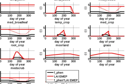
The leaf area index (LAI) is the one-sided leaf area per m2 earth surface. Since the choice of LAI-parameterization in DEPAC v.3.3 (Van Jaarsveld, 2004) was not well documented, it was decided to compare these parameterizations to those used in the EMEP model (Emberson, 2000a):

0 100 200 300 0 5 day of y ear (-) tem p_conif 0 100 200 300 0 5 day of y ear (-) tem p_decid 0 100 200 300 0 5 day of y ear (-) m ed_needle 0 100 200 300 0 5 day of y ear (-) m ed_broadleaf 0 100 200 300 0 5 day of y ear (-) tem p_crop 0 100 200 300 0 5 day of y ear (-) m ed_crop 0 100 200 300 0 5 day of y ear (-) root_crop 0 100 200 300 0 5 day of y ear (-) m oorland 0 100 200 300 0 5 day of y ear (-) grass 0 100 200 300 0 5 day of y ear (-) m edscrub latitude = 52 degrees f_phen LAI EMEP f_phen*LAI EMEP

Figure 3. Leaf area index and correction factor for phenology (reducing the stomatal conductance) during a year for EMEP land use types.

It was decided to use EMEP's parameterization for LAI in the updated DEPAC module for several reasons:

• it looks more realistic;

• it is better supported by literature;

• it has a better representation of the growing season (e.g. latitude dependent start and end of growing season).

(39)

From the above figure, we see that the growing season for temp_crop (wheat or barley) and med_crop (maize) is very short and it was decided to use the LAI for root_crop for both arable land and

permanent crop. Other parameters for the stomatal conductance are used as in temp_crop. The DEPAC land use class other uses the LAI and stomatal parameters from land use class grass.

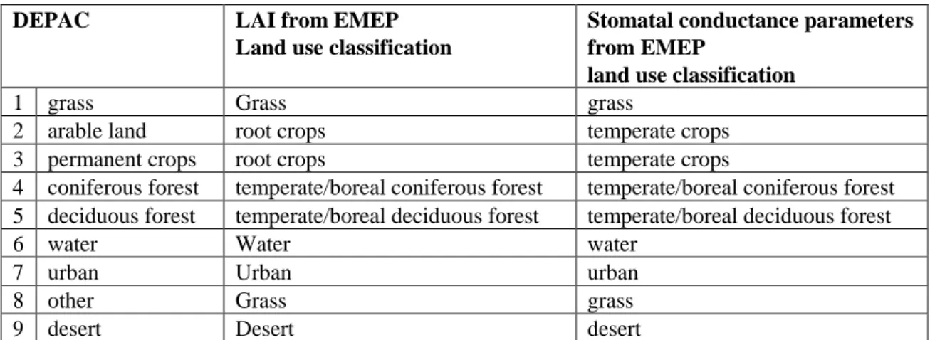
Table 5. Translation from DEPAC land use classes to EMEP.

DEPAC LAI from EMEP

Land use classification

Stomatal conductance parameters from EMEP

land use classification

1 grass Grass grass

2 arable land root crops temperate crops

3 permanent crops root crops temperate crops

4 coniferous forest temperate/boreal coniferous forest temperate/boreal coniferous forest 5 deciduous forest temperate/boreal deciduous forest temperate/boreal deciduous forest

6 water Water water

7 urban Urban urban

8 other Grass grass

9 desert Desert desert

DEPAC v.3.11 makes a distinction between the leaf area index, which is used for the stomatal resistance and the surface area index, (SAI = LAI + area index of stems and branches), which is used for the external resistance.

The following function is used to describe the temporal behavior of the leaf area index:

SGS SGS+SLEN EGS-ELEN EGS

LA I LAI_min LAI max time

Figure 4. Leaf area index as function of time. SGS: start growing season; EGS: end growing season; SLEN: length of starting phase of growing season; ELEN: length of end phase of growing season.

The start and end of growing season (SGS and EGS resp.) are dependent of the latitude λ (in degrees):

SGS(λ) = SGS(50) + ΔSGS (λ-50.0)

EGS(λ) = EGS(50) + ΔEGS (λ-50.0).

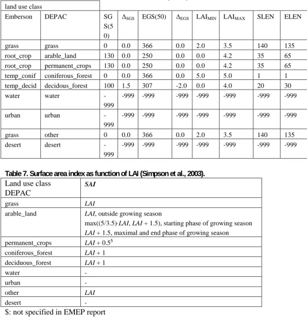
Values of SGS(50), EGS(50), ΔEGS, ΔSGS, SLEN and ELEN are given in Table 6. The surface area index

(40)

Table 6. Parameters for leaf area index from Emberson (2000a).

land use class

Emberson DEPAC SG

S(5 0)

ΔSGS EGS(50) ΔEGS LAIMIN LAIMAX SLEN ELEN

grass grass 0 0.0 366 0.0 2.0 3.5 140 135 root_crop arable_land 130 0.0 250 0.0 0.0 4.2 35 65 root_crop permanent_crops 130 0.0 250 0.0 0.0 4.2 35 65 temp_conif coniferous_forest 0 0.0 366 0.0 5.0 5.0 1 1 temp_decid decidous_forest 100 1.5 307 -2.0 0.0 4.0 20 30 water water -999 -999 -999 -999 -999 -999 -999 -999 urban urban -999 -999 -999 -999 -999 -999 -999 -999 grass other 0 0.0 366 0.0 2.0 3.5 140 135 desert desert -999 -999 -999 -999 -999 -999 -999 -999

Table 7. Surface area index as function of LAI (Simpson et al., 2003).

Land use class DEPAC

SAI

grass LAI

arable_land LAI, outside growing season

max((5/3.5)⋅LAI, LAI + 1.5), starting phase of growing season

LAI + 1.5, maximal and end phase of growing season

permanent_crops LAI + 0.5$ coniferous_forest LAI + 1 deciduous_forest LAI + 1 water - urban - other LAI desert -

$: not specified in EMEP report

In Figure 5, a comparison has been made between the EMEP and DEPAC v.3.3 parameterizations for LAI using Table 5. In the same figure, the surface area index SAI and the phenology correction factor

(41)

0 100 200 300 0 5 day of year (-) grass 0 100 200 300 0 5 day of year (-) arable land 0 100 200 300 0 5 day of year (-) permanent crops 0 100 200 300 0 5 day of year (-) coniferous forest 0 100 200 300 0 5 day of year (-) deciduous forest latitude = 52 degrees f_phen LAI EMEP SAI EMEP LAI old DEPAC f_phen*LAI EMEP f_phen*LAI old DEPAC

Figure 5. Leaf area index LAI, surface area index SAI and phenology factor fphen during a year for different land

use types, latitude = 52 degrees North. EMEP’s parameterization compared to DEPAC v.3.3. For coniferous forest, the LAI for EMEP and DEPAC v.3.3 is the same.

Since the factor fphen does not have much influence for the land use types currently used in DEPAC, it

was decided to ignore this factor. The extra factor available in the EMEP code that reduces LAI for latitudes above 60° North, has also not been included.

(42)

Appendix C. Radiation model Weiss and Norman

In order to compute the influence of solar radiation on the stomata, a simple radiation model has been employed. First we repeat some definitions from the American Meteorological Society

(http://amsglossary.allenpress.com/glossary):

solar radiation—The total electromagnetic radiation emitted by the sun. ... About one-half of the total

energy in the solar beam is contained within the visible spectrum from 0.4 to 0.7 μm, and most of the other half lies in the near-infrared, a small additional portion lying in the ultraviolet.

global radiation—Solar radiation, direct and diffuse, received from a solid angle of 2π steradians on a

horizontal surface.

direct solar radiation—Solar radiation that has not been scattered or absorbed.

In practice, solar radiation that has been scattered through only a few degrees, characteristic of the diffraction peak of the scattering function, is unavoidably included in the operational measurement of direct solar radiation by a pyrheliometer.

diffuse sky radiation—Solar radiation that is scattered at least once before it reaches the surface.

As a percentage of the global radiation, diffuse radiation is a minimum, less than 10% of the total, under clear sky conditions and overhead sun. The percentage rises with increasing solar zenith angle and reaches 100% for twilight, overcast, or highly turbid conditions. It is measured by a shadow band pyranometer.

total solar irradiance—(Abbreviated TSI.) The amount of solar radiation received outside the earth's

atmosphere on a surface normal to the incident radiation, and at the earth's mean distance from the sun. Reliable measurements of solar radiation can only be made from space and the precise record extends back only to 1978. The generally accepted value is 1368 W m−2 with an accuracy of about 0.2%. Variations of a few tenths of a percent are common, usually associated with the passage of sunspots across the solar disk. The solar cycle variation of TSI is on the order of 0.1%.

We follow Weiss and Norman (1985), the notation is however somewhat different. Characters Q, R and S are used for the radiation parameters in the radiation model:

Q : solar irradiance, on a surface normal to the incoming sun beams (W/m2);

R : potential radiation on a horizontal surface (W/m2); potential means that it occurs only in clear sky conditions;

S : actually occurring (measured) radiation on a horizontal surface; this type of radiation includes the influence of clouds (W/m2).

The following subscripts are used:

vis : visual;

ni : near-infrared;

dir : direct;

diff : diffuse.

(43)

QTSI : total solar irradiance = 1320 W/m2. C.1. The solar irradiance is split into a part in the visible wave band and a part in the near-infrared (the ultra-violet part is neglected):

TSI vis

vis

Q

=

α

,

Q

_ni

=

α

_ni

Q

_TSI , C.2.

αvis : fraction of radiation in the visible wave band = 0.46;

αni : fraction of radiation in the near-infrared wave band = 1- αvis.

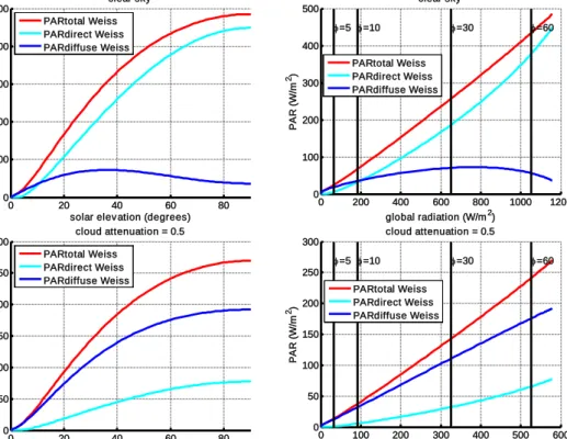
Weiss and Norman give the following parameterizations for direct and diffuse parts of visible radiation

Rvis,dir and Rvis,diff :

θ

cos

)

exp(

0 ,

m

P

K

Q

R

visdir

=

vis

−

vis C.3.

(

)

cos

θ

4 .

0

,

,diff vis visdir

vis

Q

R

=

−

C.4.

with

θ : zenith angle;

Kvis : extinction coefficient for visible radiation = 0.185;

P : pressure;

P0 : pressure at sea level (same dimension as P);

m : optical air mass,

m

=

(

cos

θ

)

−1.

The 0.4 is the fraction of intercepted visible beam radiation that is converted to downward diffuse radiation at the surface.

For near-infrared radiation:

θ

cos

)

0 exp(

,

m

w

P

K

Q

R

_ni_dir

=

_ni

−

_ni

−

C.5.

(

)

cos

θ

6 .

0

, ,

Q

R

w

R

nidiff

=

ni

−

nidir

−

C.6.

Kni : extinction coefficient for near-infrared radiation = 0.06;

w : water absorption in the near infrared for 10 mm of precipitable water

[ ]

[

2

]

10 10( )-0.0345log ( ) log 0.4459 1.1950

-10

m m TSI

Q

w

=

+ .

Adding direct and diffuse parts:

R

_vis

=

R

_vis,_dir

+

R

_vis,_diff ,

R

ni

=

R

ni,dir

+

R

ni,diff and defining ni

vis

total

R

=

+

, we have expressed all forms of potential radiation R in terms of known parameters and zenith angle θ.

It is assumed that the ratio of visible and total radiation is the same for the potential radiation and for the actually occurring radiation. Total radiation Stotal (in Weiss and Norman RT) is a quantity that is generally available as measurement or as a model result. The actually occurring visible radiation Svis can now be estimated from the total radiation by:

Description of the DEPAC module : Dry deposition modelling with DEPAC_GCN2010