Guidance for summarising earthworm field studies

Guidance for summarising earthworm field studies

F.M.W. de Jong, P. van Beelen, C.E. Smit, M.H.M.M. Montforts Corresponding author: frank.de.jong@rivm.nl

©RIVM 2006

Parts of this publication may be reproduced, provided acknowledgement is given to the ‘National Institute for Public Health and the Environment, along with the title and year of publication’.

Published by the

National Institute for Public Health and the Environment P.O. Box 1

3720 BA Bilthoven The Netherlands

This publication can be found at www.rivm.nl/bibliotheek/601506006.pdf RIVM report number 601506006/2006

ISBN 90-6960-254-0

Abstract

Guidance for summarising earthworm field studies

In order to increase the uniformity of evaluation reports, the Dutch Platform for the Assessment of Higher Tier Studies developed guidance for the evaluation of field stud-ies with earthworms.

In the framework of pesticide registration, reports of field studies (higher tier studies) with earthworms are delivered to the Competent Authorities. In the Netherlands these reports are evaluated by different Evaluating Institutes on account of the Dutch Board for the Authorisation of Pesticides (CTB). Because of the complexity of these studies, large differences occur between the evaluation reports of different institutes.

The guidance distinguishes between summarising and evaluating the study, and the use of the results in risk assessment. For summarising and evaluation a detailed guid-ance is proposed, including elaborated examples. No detailed guidguid-ance is provided here for the use of the results in risk assessment, but suggestions are given and discus-sion points are raised.

Rapport in het kort

Richtsnoer voor het samenvatten van veldstudies met regenwormen

Om de eenvormigheid van evaluaties te vergroten, en daarmee ook de inzichtelijkheid in eventuele verschillen, is door het Nederlandse Platform voor de Beoordeling van Higher Tier Studies een handleiding ontwikkeld voor het samenvatten van veldstudies met regenwormen.

Bij de registratieprocedure van bestrijdingsmiddelen worden onder meer veldstud-ies (een belangrijk voorbeeld van ‘higher tier studveldstud-ies’) aangeleverd met regenwor-men. Deze studies worden in opdracht van het College voor de Toelating van Bestrij-dingsmiddelen (CTB) geëvalueerd door verschillende experts van diverse instanties. De complexiteit van deze studies kan er toe leiden dat er grote verschillen bestaan in de vorm van de evaluaties van de verschillende instanties.

In dit rapport wordt de handleiding voor het samenvatten van deze veldstudies weerge-geven. Hierbij maakt de handleiding onderscheid tussen het samenvatten en evalu-eren van de studie zelf, naast het gebruik van de uitkomst in de risicobeoordeling. Voor het samenvatten en evalueren wordt een concrete handleiding gegeven, inclusief uitgewerkte voorbeelden. Voor het gebruik van de resultaten bij de risicobeoordeling worden slechts suggesties gegeven en discussiepunten aangereikt.

Trefwoorden: bestrijdingsmiddelen, toelating

Preface

The present guidance document is an initiative of the Dutch Platform for the Assess-ment of Higher Tier Studies. This work has been commissioned and funded by the Netherlands Ministry of Housing, Spatial Planning and the Environment in response to a request from the Board for the Authorisation of Pesticides (CTB). The aim of the Platform is to improve and harmonise the assessment of higher tier studies. The guid-ance document was drafted by a working group of the Platform. The draft report has been discussed and approved in plenary platform meetings and was finally sent out for public consultation to European experts and stakeholders. We would like to acknowl-edge Dr. A. Dintel (ECPA), Dr. A. Alix (INRA), Dr. F. Heimbach (BayerCropscience) and Dr. ir. C.A.M. van Gestel (VU-Amsterdam) for their comments on the draft report. The guidance document has been approved for publication by the plenary platform meet-ing of September 12, 2006.

For this guidance document use has been made, among others, of the technical rec-ommendations of a meeting in 2005 of experts in Lille, France (Kula et al., 2006). In this guidance document validity criteria are used in line with these recent discussions. Older studies, conducted according to guidance available at that time, cannot be ex-pected to fulfil the more recent criteria. Whether or not these studies are useful for risk assessment remains to be assessed on a case-by-case basis.

The guidance document has been presented to the Ministry of Housing, Spatial Plan-ning and the Environment, and to the Board for the Authorisation of Pesticides.

The Dutch Platform for the Assessment of Higher Tier Studies publishes practical and easy to use guidance documents for the evaluation of field effect studies and other higher tier studies. Guidance documents for summarising aquatic higher tier studies and higher tier studies on non-target arthropods are expected soon.

Bilthoven, September 2006 Dr. Mark H.M.M. Montforts Chair

Contents

Abstract ... 3

Rapport in het kort ... 5

Preface ... 7

1. Introduction ... 9

2. Guidance on summarising of test reports ... 10

3. Comments to the use of test results in risk assessment ... 18

References ... 22

1.

INTRODUCTION

In several regulatory frameworks for the authorisation of chemicals and chemical prod-ucts, such as plant protection prodprod-ucts, biocides, and veterinary medicines, higher tier studies on earthworms may be part of the dossier. These studies may be required, if the first tier risk assessment shows that the use of the product leads to an unacceptable risk for the soil compartment.

The function of a higher tier study is quite comparable in all authorisation frameworks. As an example, the Uniform Principles of EU Directive 91/414/EEC on the registration of plant protection products, appendix VI, part C paragraph 2.5.2.5 (EU, 1997) states that ‘Where there is a possibility of earthworms being exposed, no authorisation shall be granted if the acute toxicity/exposure ratio for earthworms is less than 10 or the long term toxicity/exposure ratio is less than 5, unless it is clearly established through an appropriate risk assessment that under field conditions earthworm populations are not at risk after the use of the plant protection product according to the proposed conditions of use’.

Higher tier studies on earthworms comprise mainly field studies in agricultural soil or grassland that investigate abundance and species diversity after application of the product of interest. In the EU guidance document for Terrestrial Ecotoxicology (SANCO, 2002) it is stated that an ISO method (ISO guideline 11268-3 (ISO, 1999) is available for conducting a field study, and that further information is available, with reference to Greig-Smith et al. (1992) and Sheppard et al. (1998). The described methods are not obligatory, so studies conducted according to other protocols might be acceptable as well.

Field study reports that are submitted as part of an authorisation dossier to a regula-tory authority, will be summarised and the relevant information will be presented for use in the risk assessment. This stage of dossier evaluation is performed both by industry in preparation of a monograph as part of the registration procedure under Directive 91/414/EEC, and by national authorities for national registration. This guid-ance document primarily aims to provide guidguid-ance for summarising test reports on earthworm field studies, as an integral part of the dossier evaluation process.

The purpose of the guidance is to develop a common language for summarising earth-worm field studies and for reporting those pieces of information that are relevant to decision making. This common language can be used by the scientific society dispersed over industry, academia, and authorities. The guidance also provides comments on the usefulness of these field studies for risk assessment. Therefore, a distinction is made between the assessment of the intrinsic scientific reliability of the field study and the usefulness for risk assessment.

2.

GUIDANCE ON SUMMARISING OF TEST REPORTS

The ISO guideline 11268-3 gives detailed and internationally accepted criteria for the test design. The guideline in a draft form has been used routinely (Heimbach, 1998). The last page of the ISO guideline 11268-3 states what kind of information should be available in the test reports. The current guidance document is based on the informa-tion of the ISO guideline, amended with practical experience with summarising field studies. Moreover, in May 2005, specialists from industry, registration authorities and academia met to discuss the need for updating or amending the ISO guideline (see Kula et al., 2006). The results of this discussion are incorporated in the present docu-ment. The guidance document was further discussed with Dutch experts in the Dutch Platform for the Assessment of Higher Tier Studies, and sent out to European experts for consultation. The reactions of the experts were elaborated which resulted in this final document.

When an earthworm field study is provided together with all relevant lower-tier test results, the risk assessor must verify the information presented. To that end, an evalua-tion report should be made in which the data are summarised to reach a decision in a transparent and concise way. The evaluation report has the following structure:

1. Header table or abstract, containing the decision making information on the test result and the conclusions.

2. Extended summary of the study, including test design and results, reflecting the view of the authors of the report to be evaluated.

3. Evaluation (critical comments on the test, made by the reviewer) consisting of the evaluation of the scientific reliability of the field study and the evaluation of the results of the study.

As an example, two earthworm field studies are summarised and added to the docu-ment (Annex 1), with the kind permission of the owners of the study. Because the evaluation still involves expert judgement, the discussion of the validity is not to be taken as such, but as and example how the validity should be discussed in a transpar-ent way.

The reliability is assessed by assigning a Reliability Index (Ri) to a particular test: Ri1 stands for a reliable test, Ri2 for a less reliable, and Ri3 for an unreliable test (see Table 1). The definition of reliability is: the intrinsic quality of a test with respect to the meth-odology and the description (EC, 2004). Ri3 tests are not used for risk assessment.

Table 1 Definition of the three values of the reliability index RELIABILITY

INDEX (RI)

DEFINITION DESCRIPTION

1 reliable All data are reported, the methodology and the description are in accordance with internationally accepted test guidelines and/or the instructions in this report, all other requirements fulfilled

2 less reliable Not all data reported, the methodology and/or the description are less in accordance with internationally accepted test guidelines and/or the instructions, not all other requirements fulfilled

3 not reliable Essential data missing, the methodology and/or the description are not in accordance with internationally accepted test guidelines and/or the instructions, or not reported, or important other requirements are not fulfilled

Both Ri1 and Ri2 tests can be used for risk assessment, but it depends on the overall data availability, whether only Ri1 tests should be used, or whether Ri2 tests can be used as well.

An increasing number of field studies are conducted under the principles of Good Laboratory Practice (GLP). The application of GLP puts high demands on especially the procedural aspects, and the way of reporting. This does not mean however, that studies without GLP should by definition not be used for risk assessment, or that studies under GLP can always be used.

Below a summarising table for field studies with earthworms is presented (Table 2), followed by an explanation and specification. In Appendix 1 examples of summaries of two field tests are given. The summary table is a list of items to be checked in order to reach a decision on reliability. In Table 2, an ‘E’ indicates that expert judgement should be applied to judge the impact of the shortcoming on the reliability. A ‘Y’ indicates that the shortcoming renders the test less reliable (Ri2). A combination of more Ri2 qualifications may give rise to an overall qualification as Ri3, ‘unreliable’. Some items are deemed so important for the interpretation of the test results, that a lack of such item alone renders the test not reliable (Ri3). A number of items (e.g. 2.1, 2.4) in Table 2 refer to usefulness rather than to reliability. Here it is not meant to judge the useful-ness at this point, but the items are listed to indicate that the information needed to judge the usefulness at a later stage should be reported in de summary. A reliable field study (Ri1) is not per definition useful for risk assessment. The usefulness depends on a number of other aspects, like the similarity between the test situation and the situation of the actual application, the application regime. It is also possible that a perfectly reli-able field study does not answer the particular concerns raised in the lower tiers.

Table 2 Summarising table for long-term field study with earthworms, Y = Yes, E = Expert Judgement needed

TEST ITEM NOTES RELIABILITY

LOWER?

DESCRIPTION

1. Substance improperly characterised or reported? Y [→ Ri 3]

1.1 Purity [identity and % of impurities?] Y

1.2 Formulation [formulation under consideration? identity? how much?] Y [→ Ri 3] 1.3 Vehicle [in case a vehicle – other than the formulation – is used,

identity and concentration?]

Y

2. Test site not reported Y [→ Ri 3]

2.1 Location [described in detail?] E

2.2 Field history [pesticide use, cropping system, tillage, fertilization etc.] E 2.3 Soil

type/substrate

[not reported? Organic carbon content. Field capacity, pH, particle size, profile]

Y

2.4 Crop [crop system reported?] Y

2.5 General cli-matic conditions

[not reported? necessary to make a link between the ef-fects and local climatic conditions]

E 3. Application

3.1 Mode of application

[not reported] Y [→ Ri 3]

3.2 Dosage [dosage, e.g. kg.ha-1_{] [not reported?] Y [→ Ri 3]} 3.3 Application

scheme

[not properly reported?] Y

3.4 (Micro) climate

[weather conditions before, during, and after application, rain, temperature? Irrigation?] [not reported?]

Y

4. Test design ISO 11268-3? E

4.1 Type & size [not properly reported?; plot size 10 x 10 m] Y 4.2 Test date and

duration

[duration ≥ 1 year to assess recovery] Y

4.3 Pre-treatment [pesticide use, tillage, irrigation etc shortly before treatment?] E 4.4 Negative control [if invalid] Y [→ Ri 3] 4.5 Positive control

[positive control not included (carbendazim)] Y

4.6 Replications [improper for statistical analyses] E

4.7 Statistics [improper for interpretation of results] Y [→ Ri 3] 4.8 Dose-response [not properly indicated and reported?] E 5. Biological system

5.1 Test organisms

[insufficient individuals present; adults and juveniles?] Y

TEST ITEM NOTES RELIABILITY LOWER?

6. Sampling 6.1 General features

[properties during test not properly monitored? E.g. ad-ditional pesticide treatment, tillage, fertilising, climate, irrigation]

Y

6.2 Actual concentration

[no application control, no analysis of concentration in soil?]

Y 6.3 Biological

sampling

[improper method, species, number, frequency, repli-cates, monitoring < 2 weeks before application, 1, 4 to 6 and 12 month after application]

Y

6.4 (Micro) climate

[weather conditions before and during sampling, rain, temperature? Irrigation? Soil humidity] [not reported?]

Y RESULTS

7. Application 7.1 Actual concentrations

[compound in soil not found in expected concentration] Y 7.2 Condition of

application

[no additional technical data, route under consideration] Y 7.3 Weather [extreme conditions such as long periods of drought after

application]

Y 8. Endpoint

8.1 Type [no list of earthworm species and aggregations made?] Y 8.2 Value [no list of numbers incl. s.d.; juveniles and adults,

bio-mass, all per year c.q. sampling date]

Y 8.3 Verification of

endpoint

[impossible?] E

8.4 Pre-treatment [pre-treatment variation, not limited and random?] Y 8.5 Negative

control

[low numbers? extinction] Y [→ Ri 3]

8.6 Positive control

[no or unclear effects? at least 50% effect at at least one

sample date] Y [→ Ri 3]

8.7 Weather [extreme conditions such as long periods of drought before sampling] Y 9. Elaboration of results 9.1 Statistical comparison

[improper method? Confidence level 95%, significance? Statistical power compared to results]

Y 9.2 Presentation

of results

[a graphical presentation of the results expressed as absolute and relative data is preferred]

E 9.3 Dose effect relationship [not present?] Y 9.4 Community level impact

[if given; improper method?] Y

10. Classification of effects

[not derivable?] Y

REMARKS

Item 1. Data about the substance applied and the toxic standard have to be reported in detail. For the toxic standard, the chemical analyses is not a demand.

Item 2. The history of the test site should be known (e.g. application of pesticides, mineral fertilisers, sewage sludge, etc.). Expert judgement is needed to dis-cover inconsistencies or to assess whether the field history influences the re-sult of the field study. According to ISO 11268-3, the description of the test site should include: soil profile, particle-size distribution, organic-carbon content, pH-value, moisture content at field capacity in the A-horizon and description of vegetation. General climatic conditions of the area should be presented for a number of years before the test (temperature, rainfall).

Item 3. It is important that the timing, levels and routes of exposure reflect, as far as possible, those of the proposed use of the product. Data about application are necessary for indications about exposure and extrapolation to other situ-ations. Climatic conditions in the period before, during and after the applica-tion are of importance to assess the exposure of the earthworms. A dry period might cause the earthworms to move to deeper soil layers, and might hamper the penetration of the substance into the soil. Related to this, also information about artificial irrigation should be presented. When a product is proposed to be used in autumn, the product should also be applied in autumn and the sampling scheme has to be adapted (see Item 4).

Item 4. The ISO guidance describes a number of details: a random plot design, plots of at least on hundred m2 (10 m x 10 m), with a treated 1-2 m edge strip. Four replicates should be used at least per test variant. A reference substance (posi-tive control, toxic standard) is necessary to obtain information on the effect of a test substance under the specific experimental conditions. A field applica-tion of 6 kg to 10 kg per ha of carbendazim is suitable in order to achieve sig-nificant effects of > 50% (Kula et al., 2006). According to ISO, the duration of a test should be at least 1 year, in order to assess the recovery of the earthworm community. When a compound is applied in autumn, however it is proposed to assess the recovery at the start of the next cropping season.

Item 5. A suitable test area should have an earthworm density of at least 60 indi-viduals per square metre before application. The plots should have a mixed community of species. In agricultural areas, Lumbricus spp. and Aporrectodea caliginosa or other dominant species representative for the area under study should be present at a sufficiently high density.

Item 6. When other pesticides are used before or during the test, the test results can only be used when the untreated control is treated with the same pesticides (of course not the compound under study) and shows an undisturbed develop-ment of the earthworm community, and clear effects are found in the posi-tive controls. In case the side-effects of a herbicide are studied, the untreated

control should be made free as well, for instance by mechanical weed-ing. During a recent meeting of experts (Kula et al., 2006) it was proposed to have a minimum of 60 individuals per square metre on any soil, to increase the possibility of finding statistically significant effects. The sample area for biological samples is 0.25 m2. On grassland the vegetation at the sampling area should be cut before sampling. Sampling should take place 1 month after application, 4 to 6 months after application and 12 months after application. Given the (sometimes) large variability, the pre-treatment monitoring should be conducted not too long before treatment (preferably < 2 weeks). For sam-pling of the earthworms the formaldehyde extraction method, the mustard extraction method or the electrical extraction method can be used. In all cases the efficiency of the extraction method should be checked at the beginning of each sampling period on at least three sampling areas by hand sorting. The chosen extraction method should isolate at least 60% of the hand sorted earth-worms on every sampling date. Per replicate four random samples should be taken. Adult and juvenile worms should be counted separately. Adults should be identified to the species level; juvenile worms should at least be classified as Tanylobous or Epilobous species. For enhancing the interpretation of the results a classification in epigeic (living in the superficial soil layers), endogeic (living below the soil surface in horizontal, branching burrows) and anecic (building permanent, vertical burrows) is necessary. Weather conditions in the period before sampling should be recorded. Longer periods of drought might cause the earthworms to withdraw to deeper soil layers. Key effect endpoints include (EPPO, 2003):

- Number of all earthworms and numbers of tanylobous and epilobous indi-viduals (juveniles and adults separately).

- Total biomass of all earthworms and biomass of tanylobous and epilobous individuals (juveniles and adults separately).

- Numbers of at least the two most abundant species (if possible juveniles and adults separately).

- Biomass of at least the two most abundant species (if possible juveniles and adults separately).

- Species diversity.

Concerning the species diversity it is questionable whether this is a useful pa-rameter, given the generally low number of species and individuals.

Item 7. Chemical analysis is not obligatory in the ISO guideline. However, chemical analysis of the compound in soil increases the reliability by verifying the expo-sure concentration in soil. The meaexpo-surements also facilitate the extrapolation of the results of the particular field study to other situations.

Item 8. Statistical tests can be used to determine how many replicates are actually needed given the standard error of the experiment. In some cases the varia-tion is so large that more than 4 replicates would be needed to be sure that the effect is determined with sufficient significance; in practice, an experiment has

to be planned carefully, and it is not possible to change the design on a short term. What significance level is sufficient is not clearly described. Normally a p = 0.05 is used. If the effect analysis is hampered by a given small sample size, the acceptability of a certain risk for Type I errors could be increased to for example p = 0.1 instead of p = 0.05, or the effect level of interest could be increased. Concerning the power of the test, a power of 90% respectively 95% would be logical, in analogy of the significance level. However, the traditional choice for the power is 80%. This implies that missing a relevant effect in 20% of the experiments is accepted. For both errors no values are defined in the case of field studies with earthworms. In the test report, these values should be reported explicitly.

To analyse the power of the field test, it is proposed to use the one-sided Dun-nett test (DunDun-nett, 1955, 1964, 1985). This test is the appro-priate multiple comparison method for comparing one control with several treatments if the data are normally distributed and the variance at all treatments is identical. If the number of replicas is identical in the control and in each of the treat-ments, the necessary number of replicates to reach a power P at a difference of δ is

where Φ-1 is the inverse of the cumulative standard normal distribution, σ the a priori avail-able estimate of the standard deviation and U_a,n,k the ap-propriate one-sided critical value for a test with ν degrees of freedom and k comparisons between a treatment and the control at significance level α (see Van der Hoeven, 1998).

The minimum effect level that could be determined at the given statistic sig-nificance and the control variability should be reported.

Data should be tested on normality and variance homogeneity (using Kol-mogoroff-Smirnov and Bartlett tests, respectively). Data can be logarithmically transformed to convert the Poisson distribution of the earthworm counts into a normal distribution. With normal distribution and homogeneous data, mul-tiple t-tests like Dunnett’s or William’s test should be performed. When data are not normal distributed, a multiple U-test, e.g. Bonferroni U-test, is recom-mended.

When the pre-treatment variation is large (or even significant) a comparison between treatments might be disturbed by the pre-treatment variation. In this case a correction should be made, for instance taking the pre-treatment

varia-(

)













•

Φ

•

≥

δ

σ

α, ν, k 2 -1

_(P

₎

2

+

U

2

n

tion into account as co-variate, or comparing the increase (or decrease) of the measured parameters as compared to the start between treatments.

A visual presentation in figures, plotting the numbers and biomass during time, as absolute number, or compared to the control and or the numbers present at the start of the experiment, can be of great help for interpretation of the results.

Results of the negative [untreated] control should always be regarded in detail. Due to desiccation, for instance, numbers can be very low during summer. In that case it will hardly be possible to find significant differences with treated plots. This phenomenon should not be confused with recovery, however. Clear effects should be found in the positive control, at least 50% effect at at least one sampling date. The acceptability of tests without a positive control depends on whether effects are found in the highest treatments of the com-pound under study. When no significant effects are found the test is not reli-able.

Item 9. The possible occurrence of pre-treatment variation, and large variations in time renders it necessary to present the results in different ways. As a start ab-solute differences between treatment and control should be presented. In the case of large pre-treatment variation, the presentation of relative difference (increase or decrease compared to pre-treatment) can help to get insight into the influence of pre-treatment differences.

3.

COMMENTS TO THE USE OF TEST RESULTS IN

RISK ASSESSMENT

A review showed that the relationship between laboratory toxicity and field effects is highly variable (Jones and Hart, 1998). Acute toxic effects in the field have been found both at higher and at lower concentrations than in laboratory studies. In the same re-view, a negative correlation between recovery and the persistency of the applied com-pounds was found. A field test as described in the ISO guideline 11268-3 can therefore be an important part of the higher tier risk assessment for earthworms.

However, there are a number of drawbacks that hamper the interpretation of field studies with a view to ascertain that no unacceptable effects occur under relevant field conditions. Field tests on toxicity to earthworms are very laborious since a large number of 100 m2 plots have to be monitored for a year and the earthworms have to be extracted, counted and identified down to the species level. Natural variation and low abundance in arable fields place a special effort on test design. Also variability in soil characteristics, plant cover, and humidity necessitate a considerable degree of plot replication. Converting grassland to arable land before testing superposes the effect of changing habitats on the effect of the applied compound on the earthworms. Apart from this, more limitations have been reported for field experiments (Edwards, 1998). Variability in climatic conditions can make it almost impossible to compare toxicity data on the effects of chemicals on earthworms between different seasons or regions. Currently no guidance is available concerning characteristics of the test site that should be observed, such as the organic matter content of the soil. Large differences between test conditions and the actual conditions when the product is used might result in large differences in bioavailability of the compound. Further guidance for normalisation or extrapolation of study results to realistic conditions should be developed. Therefore a single well designed field test performed according to the ISO guideline is only suf-ficient to ensure that under field conditions earthworm communities are not at risk, if additional information is presented to assess whether the field test was performed under conditions which represent a reasonable worst case estimate for the specific application at the appropriate moment in the growing season of the crop in a specific region. The same goes for persistent plant protection products. Here it depends on the dosage present in the soil during a field study whether the study can be used to assess the effects of a plateau concentration. A reference product will help determine the study validity. A thorough analyses of the exposure under test conditions and the conditions of the proposed application will also be helpful for the extrapolation of the test results.

The next question is: how much effect can be accepted, even when all conditions for this reasonable worst case situation have been fulfilled? The ISO guideline 11268-3 gives no clues how to interpret the test results in terms of unacceptable effects. In practice, even a well-performed field study according to ISO 11268-3 is not expected

to measure effects smaller than 50% with sufficient statistical confidence, although in practice some field tests with significant effects at 35% have been performed. This tech-nical restriction does not follow from a regulatory decision on acceptable effects. In the EPPO standards however some criteria are given on acceptability of effects (EPPO, 2003). The criteria given in the EPPO standard are:

“Do the results indicate that in the field, there are likely to be:

No effects > 30–50%: Categorize as low risk1

Effects > 50% observed during a study, but with full recovery within 1 year:

Categorize as medium risk

Effects > 50% without full recovery after 1 year: Categorize as high risk All other cases: Categorize as medium risk”

The EPPO documents have no formal status however, and the acceptability of 50% ef-fect, was acknowledged to be based on the limitations of the test rather then on other considerations2_{. The full recovery after 1 year is probably based on a cropping system} with a new crop in a new year. In situations where more crops are grown within one year, or where crops enter a rotation program a recovery period of one year might not be satisfactory.

To understand the implications of these boundaries of testing, it is perhaps useful to consider what actually constitutes an effect. ‘Effects’ can be defined as a statistically significant deviation from the control for any one or more of the before mentioned parameters at any time point. Whether or not one decides that a certain deviation is an effect relies upon the level of significance that can be achieved. The answer to our question of how much effect can be accepted is hence hampered beforehand by the power of the test.

Statistical confidence is a function of the desired protection against Type I and Type II errors. The Type I error occurs when an observed normal variation is classified as an effect; and the Type II error occurs when an effect is not detected. Effect size, sample size, sample variability, and accepted probabilities of Type I and Type II errors depend on each other (Sanderson and Petersen, 2002). A given small sample size automatically restricts the amount of effect that can be detected. If the lowest effect value is above the level of acceptability one prefers, the acceptability of a certain risk for Type I errors could be increased (e.g. p = 0.1 instead of p=0.05), instead of the solution that the ef-fect level of interest should be increased.

Effects at any single time point may define a short-term effect, however, the potential for recovery also needs to be considered. Based on the current test guideline ‘recovery’

1 _{Interpreted as: effects less than 30-50% represent low risk}

is indicated if significant effects compared with the control are no longer observed af-ter 1 year. There are two aspects of recovery to be considered: one is the time-frame (of 1 year), and the other is the definition of effects. Full recovery in this test type, accord-ing to EPPO criteria, means that after 1 year the effects are less than 50%, or that the effects are even above 50%, but they are not statistically significant. The EU-guidance document on Terrestrial Ecotoxicology (SANCO, 2002) does not give criteria for accept-able effects in higher tier studies. This leaves the assessor essentially with no bench-mark to determine whether no unacceptable effects will occur under field conditions. Given all uncertainties, a possible alternative solution based on the available informa-tion could be to accept the technical difficulties, and create a margin of safety:

- if effects at a dosage that is tenfold the intended field dosage are <50%: acceptable risk;

- else: unacceptable risk.

In the field trials it is much easier to measure 50% effect at 10 times the prescribed dose than finding 10% reduction at field dosage. This factor is based on field trials with benomyl where 50% reduction occurred at dosages of about 7 mg/kg dry weight soil whereas the field concentration without effect was about 10 times lower (Heimbach, 1998). This factor of 10 between the LC₅₀ and the NOEC has also been observed more often (Slooff et al., 1986; Van Gestel, 1992). Therefore the measurement of 50% inhibi-tion at 10 times the prescribed dose is considered to be a valid alternative to the NOEC at field dosage. When an effect is found, however, the applicant still has the possibility to demonstrate that the standard dose does not have unacceptable effects. Concerning recovery, inside the treated area some effects could be acceptable, meaning that recov-ery could be part of the assessment. In line with EPPO guidance in this case, earthworm community on the treated plots should be recovered one year after last application. The alternative approach proposed above is one out of more options, and should be filled in with more detail. Of course, such alternatives should only be applied when the industry foresees some favour or reduction of the workload. The intention is to show that other possibilities exist to deal with uncertainty. Recently other options like the use of TMEs (Terrestrial Model Ecosystems) are proposed, which could form a valuable intermediate between laboratory and field studies (Spurgeon et al., 2003; Weyers et al., 2004). In any case, it should be clear that the higher tier study is related to the concern that rose in the first tier, and is performed in order to lower the uncertainty factors. The discussion about effect type, acceptable effect size, sample size, and sample vari-ability, accepted probabilities of Type I and Type II errors, and the integration of dif-ferent methodologies in the decision making scheme, is however not a strict scientific one. In reaching an expert judgement on the question whether it has been demon-strated that earthworms are not at risk under field conditions, all considerations on these aspects should be worded in a transparent reasoning.

From the structure of the procedure it can be derived that the in-crop exposure and ef-fects are assessed. Whether results can be used for the assessment of off-crop exposure,

depends on the protection goals for off-crop territory. The absence of effects within the treated area (using the highest recommended dose rate) could suggest that no-effects have to be expected in off-crop area, where lower exposure is to be expected. If the absence of effects is defined as less than 50% effect, this will normally not be an accept-able effect in the off-crop situation. In field trials to assess the effects on off-crop earth-worm communities, at least the concentration to be expected should be tested, and the magnitude of the effects has to be defined. A systematic measurement of exposure in field tests should also make it easier to calculate TER values for the off-crop situation. Further work on these topics, with equal contributions from regulatory, scientific, industrial and other parties is needed.

References

Dunnett, C.W. 1955. A multiple comparison procedure for comparing several treat-ments with a control. J. Amer. Statist. Assoc. 50, 1096-1121.

Dunnett, C.W. 1964. New tables for multiple comparison with a control. Biometrics 20, 482-491.

Dunnett, C.W. 1985. Multiple comparison between several treatments and a specified treat-ment. In: Linear Statistical Inference (ed. T. Calinski & W. Klonecki), Lecture Notes in Statistics, Vol 35: 39-47.

EC. 2004. European Union System for the Evaluation of Substances 2.0 (EUSES 2.0). Prepared for the European Chemicals Bureau by the National Institute for Public Health and the Environment (RIVM), Bilthoven, The Netherlands. Available via the ECB, http://ecb.jrc.it,

Edwards, C.A. 1998. Principles for the design of flexible earthworm field toxicity exper-iments and interpretation of results. In: Sheppard, S.C., Bembridge, J.D., Holmstrup, M. and Posthuma, L. (Eds.) Advances in earthworm ecotoxicology. Proceedings from the second international workshop on earthworm ecotoxicology, 313-326. Amster-dam, SETAC press, SETAC, Pensacola, FL.

EPPO. 2003. Environmental risk assessment scheme of plant protection products. Chap-ter 8: Soil organisms and functions. EPPO Bulletin 33, 195-209.

EU. 1997. Doc. 397L0057. Council Directive 97/57/EC of 22 September 1997 establish-ing Annex VI to Directive 91/414/EEC concernestablish-ing the placestablish-ing of plant protection products on the market. Official Journal L265, 0087-0109.

Greig-Smith, P.W., Becker, H., Edwards, P.J. and Heimbach, F. 1992. Ecotoxicology of earthworms, Hants, United Kingdom: Intercept Ltd.

Heimbach, F. 1998. Comparison of the sensitivities of an earthworm (Eisenia fetida) reproduction test and a standardised field test on grassland. In: Sheppard, S.C., Bembridge, J.D., Holmstrup, M. and Posthuma, L. (Eds.) Advances in earthworm ecotoxicology. Proceedings from the second international workshop on earthworm ecotoxicology, 235-245. Amsterdam, SETAC press, SETAC, Pensacola, FL.

ISO. 1999. ISO 11268-3. Soil quality - effects of pollutants on earthworms. Part 3: Guid-ance on the determination of effects in field situations.

Jones, A. and Hart, A.D.M. 1998. Comparison of laboratory toxicity tests for pesticides with field effects on earthworm populations: a review. In: Sheppard, S.C., Bembridge, J.D., Holmstrup, M. and Posthuma, L. (Eds.) Advances in earthworm ecotoxicology. Proceedings from the Second International Workshop on Earthworm Ecotoxicology, Amsterdam, p. 247-267. SETAC, Pensacola FL.

Kula, C., Heimbach, F., Riepert, F. and Römbke, J. 2006. Technical recommendations fort he update of the ISO earthworm field test guideline (ISO 11268-3). Journal of Soils and Sediments 6, 182-186.

SANCO. 2002. Guidance document on terrestrial ecotoxicology under council directive 91/414. Draft Working Document. EU (DG Health and Consumer Protection), Brus-sels, Belgium. SANCO/1039/2002 rev 2 final.

Sanderson, H. and Petersen, S. 2002. Power analysis as a reflexive scientific tool for inter-pretation and implementation of the precautionary principle in the European Union. Environmental Science and Pollution Research 9, 221-226.

Sheppard, S.C., Bembridge, J.D., Holmstrup, M. , and Posthuma, L. 1998. Advances in earthworm ecotoxicology. Proceedings from the Second International Workshop on Earthworm Ecotoxicology, Amsterdam, SETAC Press. SETAC, Pensacola FL.

Slooff, W., Van Oers, J.A.M. and De Zwart, D. 1986. Margins of Uncertainty in Ecotoxico-logical Hazard Assessment. Environmental Toxicology and Chemistry 5, 841-852. Spurgeon, D.J., Week, J.M. and Van Gestel, C.A.M. 2003. A summary of eleven years

progress in earthworm ecotoxicology. Pedobiologia 47, 558-606.

Van der Hoeven, N. 1998. Power analysis for the NOEC: What is the probalility of de-tecting small toxic effects on three different species using the appropriate standard-ized test protocols? Ecotoxicology 7, 355-361.

Van Gestel, C.A.M. 1992. Validation of earthworm toxicity tests by comparison with field studies: a review of benomyl, carbendazim, carbofuran, and carbaryl. Ecotoxi-cology and Environmental Safety 23, 221-236.

Weyers, A., Sokull-Klüttgen, B., Knacker, T., Martin, S. and Van Gestel, C.A.M. 2004. Use of terrestrial model ecosystem data in environmental risk assessment for industrial chemicals, biocides and plant protection products in the EU. Ecotoxicology 13, 163-176.

ANNEX 1. EXAMPLES OF SUMMARIES

Disclaimer: the summaries of the field studies as presented below are examples of summa-ries following the guidance presented in this book. The studies were used and rendered anonymous with kind permission of the owner of the studies. No rights can be founded on the conclusions of these evaluations presented here.

Earthworm field study 1

1.

Header Table

reference : XXXX GLP statement : Yes

type of study : Earthworm field study guideline : in accordance BBA VI (1994) and ISO 11628-3, 1999 year of execution : 2002-2003 acceptability : Acceptable

test substance : formulation

Sub-stance Species Lo- ca-tion Soil type OM [%] Dose [g as/ ha] Time of appli-cation Duration [months] Criterion Signifi-cant effects > 50 % Y/N Recovery after 1 year Y/N Ri XXXX earthworm field fauna xxxx, D loamy sand 2.3 – 2.7 N 7 June 2002 12 abundance biomass N N - 2 2.3 – 2.7 2N 7 June 2002 12 abundance biomass N N - 2 2.3 – 2.7 4N 7 June 2002 12 abundance biomass N N - 2 2.3 – 2.7 8N 7 June 2002 12 abundance biomass Y Y N N 2 Reference XXXX

2.

Extended summary

Guidelines BBA VI (1994), ISO 11628-3, 1999. Test substance

Test site and maintenance

The test was performed from June 2002 until June 2003 on a red fescue field near XXXX, Germany. The soil type was loamy sand (USDA), OM content 2.3 – 2.7 %, pH-CaCl₂ 5.5 – 5.7, CEC reported as 69 mmol/kg (see Remarks), WHC 30.6 – 37.1 %. The field had a cultivation history of winter barley in 1999, winter wheat in 2000, triticale in 2001 and spring barley in 2002. Previously applied pesticides include diflufenican, isoproturon, carbendazim, flusiolazole and azoxystrobin in 1999, diflufenican, isoproturon, chlormequat, trinexa-pac, fenpropimorph, epoxiconazole, kresoxim-methyl en fenpropidin in 2000, diflufeni-can, isoproturon, azoxystrobin, chlormequat and trinexapac in 2001 and dichlorprop-P and tribenuron in 2002. NP(K)-fertilisers were applied each year. No pesticides or fertilis-ers were applied since the start of the study. Red fescue was sown in September 2002. On 8 and 9 June 2002 (1 – 2 days after application), the site was irrigated with a total of 18 and 18.5 mm. Additional irrigation (75 mm total) was applied before the last sampling in June 2003.

Application, replicates

Application took place on 7 June 2002, using a tractor mounted field sprayer with a spray-ing boom of 9.5 m and a total of 19 Lechler LU120-05 nozzles (spacspray-ing 0.5 m). Control, nominal application rates 1N, 2N, 4N and 8N (where N = normal application rate) as/ha and a toxic reference (carbendazim, 4 kg as/ha) were sprayed with a water volume of 300 L/ha. Four replicate plots (15 x 19 m2_{) per treatment. Weather conditions during} applica-tion were 15 – 16 °C, wind speed 0.3 – 1.3 m/s.

Earthworm sampling

Sampling of earthworms took place 1 to 2 days before treatment and after ca. 2, 4, 6, 10 and 13 months (53, 109, 179, 312 and 381 days). On each sampling occasion, four sub-plots of 0.25 m2 _{per plot were sampled by a combination of hand-sorting and formalin} extraction. Efficiency was checked by hand sampling on every sampling occasion and was between 79 and 87 %, 42.5 % efficiency was recorded at the last sampling date. Sub-samples were combined and worms were identified to the species level (some juveniles to the genus level) and numbers and weight were recorded. Additional surface searching was carried out within four 1 m2 _{quadrates in each plot on days 1 to 9 after application,} the same area was used each day.

Analytical verification

Soil. Soil samples were collected 3, 5 and 6 days after application. Soil cores (2.5 cm ø, 20

cm deep) were collected, 20 cores per plot. Cores were frozen and cut into 0 – 1, 1 – 3, 3 – 5, 5 – 10 and 10 – 20 cm layers or into 0 – 5, 5 – 10 and 10 – 20 cm segments, corresponding segments were pooled and homogenised. Soil was extracted by shaking with acetone:0.1 M HCl (75:25 v/v), aliquots of the extracts were diluted with ultrapure water and analysed with HPLC-MS-MS. LOQ was 0.01 mg/kg, recovery of fortified samples 78 - 111 %.

Earthworms. Earthworms found on the surface of the treated plots were collected 3 to 11

days after treatment. Worms were frozen and stored until analysis. Control worms were obtained from a breeding culture because no control worms from the test site were sup-plied. Extraction and analysis of worms was as described above for soil, with addition of

filtration over 0.45 µm filter discs after extraction. LOQ 0.1 mg/kg, recovery of fortified samples was 65 – 88 % (mean 73 and 79 %).

Statistical evaluation

Mean numbers and abundance were analysed by ANOVA (pre-application) or by ANCOVA with F-test (post-treatment) using the pre-treatment results as a co-variate. If the co-vari-ate was not significant, ANOVA was used. The pooled estimco-vari-ate of residual error variance was used to compare each treatment to the control using a two-sided Dunnett’s t-test. Abundance data were log (n +1) transformed before analysis. P was < 0.05.

Results

Environmental conditions

Total natural precipitation fluctuated and relatively wet months alternated with dry peri-ods. A summary of rainfall and temperature data is given in Table 1.

Table 1. Rainfall and temperature during study

Month Rainfall at site [mm] Long-term average [mm] Rainfall at site relative to long-term average [%] Average air tempera-ture [°C] Long-term average [°C] June 2002 (application 7/6) 90.2 74 +22 16.1 15.5 July 2002 (sampling 30-31/7) 175.8 82 +114 17.3 16.8 August 2002 80.2 70 +15 19.9 16.6 September 2002 (sampling 24-25/9) 23.4 70 -67 14.5 13.5 October 2002 132.4 63 +110 7.7 9.7 November 2002 79.6 71 +12 4.6 5.1 December 2002 (sampling 34/12) 34.8 72 -52 -0.9 1.9 January 2003 77.2 61 +27 0.0 0.5 February 2003 16.2 41 -60 -1.0 1.1 March 2003 40.8 56 -27 4.9 3.7 April 2003 (sampling 15-16/4) 51.7 51 +1 8.6 7.3 May 2003 92.4 57 +62 13.0 12.2 June 2003 (sampling 23-24/6) 8.4 74 -89 17.5 15.5

Volumetric water content at 20 cm depth was between 8 % in June 2003 and 44 % in November 2002. Average daily soil temperature ranged from -1.3 to 22.4 °C.

Residue analysis

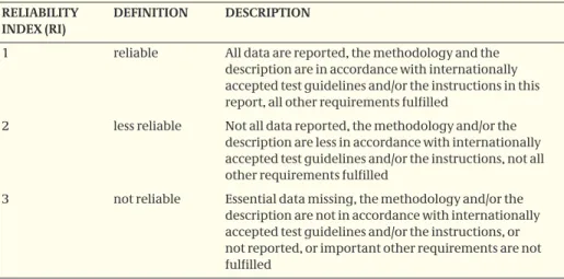
Soil. Soil analysis data are summarised in the Table 2 below, all values were corrected for

recovery when mean concurrent recovery was < 100 %. Table 2. Mean residues of YYYY in soil

Treat-ment [g as/ha]

Time [DAT]1 Soil_layer

[cm] Residue [mg/kg dwt] Residue [% of nomi-nal]2 Treat-ment [g as/ha] Time [DAT]1 Soil_layer

[cm] Residue [mg/kg dwt] Residue [% of nomi-nal]2 control 2 0 - 10 < 0.01 4N 2 0 – 5 0.18 54 N 2 0 – 1 0.18 41 5 – 10 0.02 4 1 – 3 0.02 7 4 0 – 5 0.19 58 > 3 < 0.01 5 – 10 < 0.01 4 0 – 5 0.04 50 6 0 – 5 0.19 54 5 – 10 < 0.01 5 – 10 < 0.01 6 0 – 1 0.13 29 8N 2 0 – 5 0.32 45 1 – 3 0.02 8 5 – 10 0.01 2 > 3 < 0.01 4 0 – 5 0.36 53 2N 3 0 – 1 0.36 40 5 – 10 0.02 3 1 – 3 0.04 8 6 0 – 1 1.54 37 > 3 < 0.01 1 – 3 0.20 11 4 0 – 5 0.11 62 3 – 5 0.05 3 5 – 10 < 0.01 5 – 10 0.02 4 6 0 – 1 0.33 35 1 – 3 0.05 10 3 – 5 0.02 3 > 5 < 0.01 1: Days After Treatment

2: Nominal is based on total amount applied on the surface of 20 cores and the dry weight of the respective soil layers

Earthworms. Mean residues are shown in Table 3 below.

Table 3. Mean residues of YYYY in dead earthworms

Treatment Residue in earthworms [mg/kg wwt] at each sampling interval [DAT]1

2 3 4 5 6 7 8 control < 0.12 1N 2.2 2.4 1.6 - - - -2N 2.7 2.0 1.6 1.3 - - -4N 2.9 2.2 2.4 2.3 1.1 1.6 -8N 4.8 3.2 2.5 2.6 1.5 3.5 3.1

1: Days After Treatment 2: combined sample

Biological system

A total of nine taxa was identified; adults were classified as anecic (Lumbricus terrestris) and endogeic (Aporrectodea caliginosa, A. rosea, Allolobophora chlorotica and Octalosion cyaneum). Juveniles were identified as A. caliginosa, A. chlorotica, Lumbricus spp., Octalo-sion spp. and epilobous species being mainly Aporrectodea. In the pre-treatment samples, total numbers of worms per m2 _{were between 69 and 74, the majority being juveniles and} adults of A. caliginosa, A. chlorotica and L. terrestris.

Surface searching. The cumulative mean number of earthworm found dead or dying at

the surface over the first 9 days after application increased from 4.0 per m2 _{at N as/ha to} 18 per m2 _{at 8N as/ha. Expressed as percentage of the pre-treatment abundance, the} cu-mulative effect percentage at 8N as/ha was 25.4 %. Lumbricus was relatively most sensitive (42 % mortality of adults and juveniles as compared to pre-treatment numbers), endogeic species were less sensitive (20 % mortality). Juvenile mortality was 29 % as compared to pre-treatment numbers.

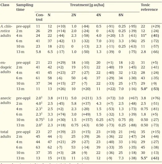
Table 4. Abundance of adult earthworms over time, values represent mean number of worms/m2_.

Values between parentheses are relative differences to the control in % Class Sampling

time

Treatment [g as/ha] Toxic

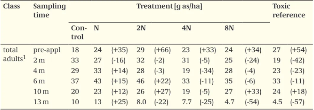
reference Con-trol N 2N 4N 8N A. chlo-rotica adults pre-appl 2 m 4 m 11 26 24 12 29 22 (+10) (+14) (-44) 1.0 2.0 2.3 (-84) (-24) (-58) 0.5 0 4.0 (-91) (-63) (+20) 0.25 0.25 1.5 (-95) (-39) (-61) 22 12 11* (+29) (-24) (-81) 6 m 41 37 (-42) 13 (-32) 7.0 (-31) 3.3 (-56) 25 (-72) 10 m 23 18 (-21) 0 (-13) 2.3 (-11) 0.25 (-63) 11 (-57) 13 m 5.8 6.5 (-17) 1.0 (-50) 1.3 (-39) 0 (-75) 2.8 (-66) en-dogeic adults pre-appl 2 m 21 41 23 42 (+29) (+2) 18 19 (-10) (-51) 20 22 (+1) (-40) 18 19 (-2) (-45) 31 22 (+5) (-41) 4 m 41 45 (+23) 27 (-27) 22 (-40) 32 (-12) 28 (-24) 6 m 61 58 (-6) 50 (-4) 37 (-29) 34 (-30) 43 (-35) 10 m 37 34 (+15) 27 (-7) 22 (-33) 25 (-17) 29 (-9) anecic adults 13 m pre-appl 11 2.01 13 3.8 (+26) (+111) 10 5.0 (+20) (+211) 11 3.5 (+22) (+72) 7.0 3.0 (-16) (+67) 5.0* 3.8 (-53) (+76) 2 m 4.01 _{2.5 (-45) 5.8 (+37) 4.3 (+7) 2.5 (-48) 2.5 (-51)} 4 m 2.31 _{2.5 (+2) 2.3 (-20) 1.5 (-53) 1.3 (-73) 0.75 (-81)} 6 m 2.31 _{3.3 (+74) 3.0 (+49) 1.5 (-32) 1.3 (-39) 1.8 (+5)} 10 m 0.751 _{1.0 (+30) 1.5 (+157) 0.25 (-67) 0.75 (0) 0.50 (-27)} 13 m 2.01 _{2.3 (+18) 0.75 (-63) 0.50 (-73) 0.25 (-88) 0.50 (-73)} total adults pre-appl 2 m 23 45 27 44 (+39) (-1) 23 25 (+15) (-39) 23 26 (+10) (-36) 21 22 (+6) (-47) 35 24 (+15) (-44) 4 m 44 47 (+21) 29 (-27) 23 (-40) 33 (-16) 29 (-27) 6 m 63 62 (-7) 53 (-14) 39 (-33) 35 (-35) 45 (-38) 10 m 37 35 (+3) 28 (-9) 22 (-36) 25 (-18) 30 (-13) 13 m 13 15 (+13) 11 (-12) 12 (-9) 7.3 (-38) 5.5* (-61)

1: numbers in control too low for statistical analysis

Abundance. Mean numbers of earthworms per sampling date are given in Tables 4 to

6 for adults and juveniles and the total earthworm community. Significant differences from the control are indicated by asterisks, statistical analysis was only performed when mean abundance in the control was > 5/m2_{. Relative differences to the control are given} between parentheses, percentages are based on back-transformed numbers and adjust-ed for pre-treatment differences when appropriate.

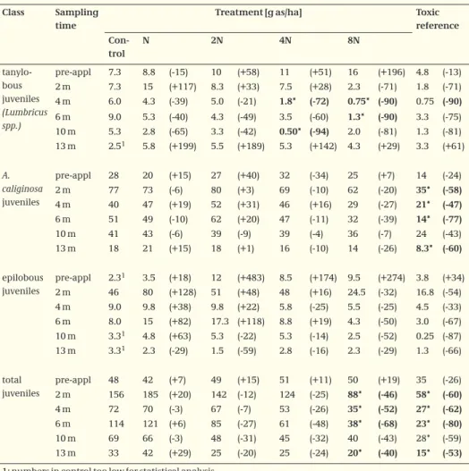
Table 5. Abundance of juvenile earthworms over time, values represent mean number of worms/m2_.

Values between parentheses are relative differences to the control in %

Class Sampling time

Treatment [g as/ha] Toxic reference Con-trol N 2N 4N 8N tanylo-bous juveniles (Lumbricus spp.) pre-appl 7.3 8.8 (-15) 10 (+58) 11 (+51) 16 (+196) 4.8 (-13) 2 m 7.3 15 (+117) 8.3 (+33) 7.5 (+28) 2.3 (-71) 1.8 (-71) 4 m 6.0 4.3 (-39) 5.0 (-21) 1.8* (-72) 0.75* (-90) 0.75 (-90) 6 m 9.0 5.3 (-40) 4.3 (-49) 3.5 (-60) 1.3* (-90) 3.3 (-75) 10 m 5.3 2.8 (-65) 3.3 (-42) 0.50* (-94) 2.0 (-81) 1.3 (-81) 13 m 2.51 _{5.8 (+199) 5.5 (+189) 5.3 (+142) 4.3 (+29) 3.3 (+61)} A. caliginosa juveniles pre-appl 28 20 (+15) 27 (+40) 32 (-34) 25 (+7) 14 (-24) 2 m 77 73 (-6) 80 (+3) 69 (-10) 62 (-20) 35* (-58) 4 m 40 47 (+19) 52 (+31) 46 (+16) 29 (-27) 21* (-47) 6 m 51 49 (-10) 62 (+20) 47 (-11) 32 (-39) 14* (-77) 10 m 41 43 (-6) 39 (-9) 39 (-4) 36 (-7) 24 (-43) 13 m 18 21 (+15) 18 (+1) 16 (-10) 14 (-26) 8.3* (-60) epilobous juveniles pre-appl 2.31 _{3.5 (+18) 12 (+483) 8.5 (+174) 9.5 (+274) 3.8 (+34)} 2 m 46 80 (+128) 51 (+48) 48 (+16) 24.5 (-32) 16.8 (-54) 4 m 9.0 9.8 (+38) 9.8 (+22) 5.8 (-25) 5.5 (-25) 4.5 (-33) 6 m 8.0 15 (+82) 17.3 (+118) 8.8 (+19) 4.3 (-50) 3.0 (-67) 10 m 3.31 _{4.8 (+63) 5.3 (-22) 5.3 (-14) 2.5 (-52) 0.25 (-87)} 13 m 3.31 _{2.3 (-29) 1.5 (-59) 2.8 (-16) 2.3 (-29) 1.3 (-66)} total juveniles pre-appl 48 42 (+7) 49 (+15) 51 (+11) 50 (+19) 35 (-26) 2 m 156 185 (+20) 142 (-12) 124 (-25) 88* (-46) 58* (-60) 4 m 72 70 (-3) 67 (-7) 53 (-26) 35* (-52) 27* (-62) 6 m 114 121 (+6) 85 (-27) 61 (-48) 38* (-68) 23* (-80) 10 m 69 66 (-3) 48 (-31) 45 (-32) 40 (-43) 28* (-59) 13 m 33 42 (+29) 25 (-20) 25 (-24) 20* (-40) 15* (-53)

1: numbers in control too low for statistical analysis

Table 6. Abundance of total earthworms over time, values represent mean number of worms/m2_{. Values}

between parentheses are relative differences to the control in % Class Sampling

time

Treatment [g as/ha] Toxic

reference Con-trol N 2N 4N 8N all worms pre-appl 71 69 (+18) 71 (+16) 74 (+10) 71 (+15) 69 (-12) 2 m 201 230 (+12) 167 (-8) 150 (-27) 110* (-46) 82* (-59) 4 m 116 117 (+4) 95 (-15) 76* (-32) 68* (-40) 56* (-51) 6 m 178 183 (0) 137 (-20) 99* (-43) 72* (-58) 68* (-65) 10 m 106 101 (-3) 76 (-26) 67 (-35) 66 (-37) 58* (-42) 13 m 45 56 (+26) 36 (-17) 36 (-20) 27* (-39) 20* (-54)

*: Significantly different from control (analysis performed with transformed data)

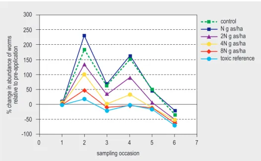
Changes in abundance of the total earthworm community over time are presented in Figure 1, based on absolute numbers (Fig. 1a), change relative to pre-treatment sampling (Fig. 1b) and change relative to control (Fig. 1c). Figures are prepared by evaluator, based on absolute numbers from Table 6.

Figure 1a. Total abundance of earthworms on the different sampling occasions. (occasion 1 is pre-treatment sampling).

total # of worms/m 2 100 0 0 1 150 200 250 50 7 6 5 4 3 2 sampling occasion control N g as/ha 2N g as/ha 4N g as/ha 8N g as/ha toxic reference

Figure 1b. Total abundance of earthworms on the different sampling occasions, relative to pre-treatment sampling (sampling occasion 1).

Figure 1c. Total abundance of earthworms on the different sampling occasions, relative to control (X-axis).

0 1 2 3 4 5 6 7

sampling occasion

% change in abundance of worms

relative to pre-application 50 -100 150 100 250 300 200 -50 0 control N g as/ha 2N g as/ha 4N g as/ha 8N g as/ha toxic reference 0 1 2 3 4 5 6 7 sampling occasion % di

fference in abundance of worm

s relative to control -40 -80 -20 20 40 -60 0 0 N g as/ha 2N g as/ha 4N g as/ha 8N g as/ha toxic reference

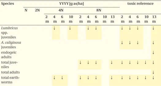
A summary of significant differences in abundance of the identified species and classes is given in Table 7.

Table 7. Significant differences in abundance of earthworms, ↓ indicates decrease, ↑ indicates increase.

Species YYYY [g as/ha] toxic reference

N 2N 4N 8N 2 m 4 m 6 m 10 m 2 m 4 m 6 m 10 m 13 m 2 m 4 m 6 m 10 m 13 m Lumbricus spp. juveniles ↓ ↓ ↓ ↓ ↓ ↓ ↓ ↓ A. caliginosa juveniles ↓ ↓ ↓ ↓ endogeic adults ↓ total juve-niles ↓ ↓ ↓ ↓ ↓ ↓ ↓ ↓ ↓ total adults ↓ total earth-worms ↓ ↓ ↓ ↓ ↓ ↓ ↓ ↓ ↓ ↓ ↓

Biomass. Mean biomass of earthworms per sampling date are given in Tables 8 to 10 for

adults and juveniles and the total earthworm community. Significant differences are indicated by asterisks. Relative differences to the control, after adjustment for pre-treat-ment differences when appropriate, are given between parentheses.

Table 8. Mean biomass of adult earthworms over time, values represent g/m2_{. Values between}

parenthe-ses are relative differences to the control in %. Class Sampling

time

Treatment [g as/ha] Toxic

reference Con-trol N 2N 4N 8N en-dogeic adults pre-appl 9.0 12 (+29) 12 (+36) 13 (+41) 14 (+54) 12 (+33) 2 m 18 17 (-6) 13 (-29) 17 (-8) 16 (-13) 11 (-41) 4 m 20 24 (+23) 20 (+1) 14 (-27) 25 (+27) 20 (+1) 6 m 30 30 (+2) 35 (+19) 28 (-6) 31 (+3) 27 (-9) 10 m 17 18 (+11) 21 (+28) 18 (+9) 23 (+39) 21 (+29) 13 m 3.3 4.0 (+19) 4.8 (+44) 5.7 (+72) 3.8 (+14) 1.9 (-44) anecic adults pre-appl 2 m 8.5 14 12 10 (+41) -28) 17 19 (2) (+32) 11 14 (+24) (-2) 9.6 8.8 (+13) (-38) 15 8.2 (+75) (-42) 4 m 9.7 9.3 (-5) 8.6 (-12) 5.2 (-46) 3.2 (-67) 2.8 (-71) 6 m 7.8 13 (+67) 10 (+30) 5.3 (-31) 4.7 (-40) 6.2 (-20) 10 m 3.7 4.4 (+18) 4.6 (-23) 1.1 (-69) 3.8 (+3) 2.5 (-33) 13 m 6.9 8.8 (+27) 3.2 (-54 2.0 (-71) 0.89 (-83) 2.6 (-67)

Table 8. Mean biomass of adult earthworms over time, values represent g/m2_{. Values between}

parentheses are relative differences to the control in %. Class Sampling

time

Treatment [g as/ha] Toxic

reference Con-trol N 2N 4N 8N total adults1 pre-appl_{2 m} 18₃₃ 24₂₇ (+35)_(-16) 29_{32 (-2)}(+66) ₃₁23 _(-5)(+33) ₂₅24 _(-24)(+34) ₁₉27 (+54)_(-42) 4 m 29 33 (+14) 28 (-3) 19 (-34) 28 (-4) 23 (-23) 6 m 37 43 (+15) 46 (+22) 33 (-11) 35 (-6) 33 (-11) 10 m 20 23 (+12) 26 (+27) 19 (-5) 27 (+33) 24 (+18) 13 m 10 13 (+25) 8.0 (-22) 7.7 (-25) 4.7 (-54) 4.5 (-57)

1: differences due to rounding off

Table 9. Mean biomass of juvenile earthworms over time, values represent g/m2_{. Values between}

parentheses are relative differences to the control in %.

Class Sampling time

Treatment [g as/ha] Toxic

reference Con-trol N 2N 4N 8N tany-lobous juveniles (Lumbri-cus spp.) pre-appl 7.5 11 (+43) 7.6 (+1 13 (+79) 16 (+116) 4.1 (-46) 2 m 4.0 10 (+163) 7.2 (+81) 7.9 (+97) 1.8 (-55) 1.6 (-59) 4 m 4.9 4.2 (-14) 6.0 (+22) 2.2 (-55) 0.96 (-81) 0.63 (-87) 6 m 3.3 4.9 (+48) 1.6 (-52) 1.9 (-64) 0.40 (-88) 1.4 (-52) 10 m 1.4 0.49 (-65) 1.4 (+) 0.08 (-94) 0.72 (-49) 0.47 (-67) 13 m 1.6 3.9 (+138) 4.1 (+148) 1.8 (+8) 1.4 (-14) 2.4 (+49) epilo-bous juveniles pre-appl 0.24 0.35 (+49) 2.6 (+986) 1.4 (+512) 1.4 (+504) 0.64 (+169) 2 m 2.7 5.0 (+86) 4.8 (+79) 4.3 (+59) 2.6 (-3) 1.6 (-42) 4 m 1.5 1.5 (-6) 1.5 (-6) 0.67 (-53) 0.90 (-42) 1.0 (-32) 6 m 1.1 1.5 (+44) 2.2 (+108) 0.72 (-32) 0.43 (-60) 0.49 (-54) 10 m 0.28 0.59 (+110) 0.92 (+227) 0.86 (+203) 0.20 (-30) 0.01 (-95) 13 m 0.30 0.20 (-32) 0.10 (-67) 0.29 (-3) 0.19 (-38) 0.02 (-92) total ju-veniles1 pre-appl 16 17 (+7) 17 (+9) 23 (+49) 25 (+60) 10 (-36) 2 m 29 39 (+29) 38 (+29) 38 (+28) 27 (-8) 17 (-41) 4 m 17 18 (+7) 22 (+26) 16 (-9) 8.0* (-53) 8.5 (-50) 6 m 25 26 (+5) 25 (-2) 17 (-34) 11* (-57) 7.8* (-69) 10 m 17 17 (+1) 16 (-5) 15 (-14) 13 (-26) 9.4 (-45) 13 m 6.0 9.4 (+57) 8.1 (+36) 5.8 (-2) 4.7 (-22) 4.2 (-30)

1: differences due to rounding off *: Significantly different from control

Table 10. Mean biomass of total earthworms over time, values represent g/m2_{. Values between}

parentheses are relative differences to the control in %. Class Sampling

time

Treatment [g as/ha] Toxic

reference Con-trol N 2N 4N 8N all worms pre-appl 33 40 (+22) 46 (+39) 47 (+40) 48 (+46) 37 (+11) 2 m 62 65 (0) 70 (+1) 68 (0) 52 (-27) 36* (-42) 4 m 47 52 (+11) 50 (+8) 35 (-25) 36 (-22) 31 (-33) 6 m 63 69 (+11) 70 (+12) 50 (-20) 46 (-26) 41 (-34) 10 m 38 40 (+70 42 (+12) 34 (-9) 40 (+6) 33 (-11) 13 m 16 22 (+37) 16 (-1) 14 (-17) 9.4 (-42) 8.6 (-47)

*: Significantly different from control

Changes in biomass of total earthworms over time are presented in Figure 2, based on absolute weights (Fig. 2a), change relative to pre-treatment sampling (Fig. 2b) and change relative to control (Fig. 2c). Figures are prepared by evaluator, based on absolute data in Table 10.

Figure 2a. Total biomass of earthworms on the different sampling occasions (occasion 1 is pre-treatment sampling).

total biomass of worms [g/m

2] 40 0 0 1 60 70 80 100 90 50 20 30 10 7 6 5 4 3 2 sampling occasion control N g as/ha 2N g as/ha 4N g as/ha 8N g as/ha toxic reference

Figure 2b. Total biomass of earthworms on the different sampling occasions, relative to pre-treatment sampling (sampling occasion 1)

Figure 2c. Total biomass of earthworms on the different sampling occasions, relative to control (X-axis).

A summary of significant differences in biomass of the identified species and classes is given in Table 11.

% change in biomass of worms relative to pre-application -40

-100 40 20 80 100 60 -60 -20 -80 0 control N g as/ha 2N g as/ha 4N g as/ha 8N g as/ha toxic reference 0 1 2 3 4 5 6 7 sampling occasion % dif

ference in biomass of worms relative to control -20

-60 0 40 60 -40 20 N g as/ha 2N g as/ha 4N g as/ha 8N g as/ha toxic reference 0 1 2 3 4 5 6 7 sampling occasion

Table 11. Significant differences in biomass of earthworms, ↓ indicates decrease

Species YYYY [g as/ha] toxic reference

N 2N 4N 8N 2 m 4 m 6 m 2 m 4 m A. caliginosa juveniles ↓ total juveniles ↓ ↓ ↓ total earthworms ↓

Authors conclude that a single application of 4N and 8N g as/ha results in initial signifi-cant effects on the earthworm field fauna. Signifisignifi-cant effects > 50 % were observed at 8N g as/ha, and full recovery was not observed within a year (40 % reduction after 13 months). At the last sampling date, sampling efficiency was only 42.5 %, which may have affected the results.

3.

Evaluation

Average CEC was reported as 6.9 cmol/kg (69 mmol/kg), values from individual samples ranged from 17 to 167 mmol/kg (n = 6). Other soil characteristics that may influence CEC (OM- and clay content, pH) do not show such a large variation, and the reported CEC val-ues may be incorrect. This is not considered to have influenced the outcome of the study. Residue levels in worms on treated plots were compared with residue levels of the breed-ing culture rather than worms from the control plot. Therefore the validity of the analysis in worms is questionable.

A. chlorotica was found in high numbers in some plots, while the species was not present in others. It appears that the plots where A. chlorotica was present are all located in the same corner of the test field. The absence of this species in the other plots may be due to previous cultivation practices, including the use of pesticides that are known to be harm-ful to earthworms (e.g. carbendazim).

Short term effects are only assessed by looking for dead earthworms at the surface, and the first full biological assessment is two months after application. Nevertheless, there is a clear trend towards a decrease in abundance at application rates of 2N as/ha and higher, although differences at 2N as/ha are not significant. Reductions at 4N as/ha are significant, but < 50 %. Changes in biomass are less apparent, significant differences were only found at 8N as/ha. Full recovery at 8N as/ha after 13 months is not demonstrated, although no significant reductions were present at the preceding sampling data after 10 months in April 2003. The latter may be due to the relatively dry conditions in February and March 2003, causing a generally lower abundance and thereby a higher variability between the plots. From the results of the study it can be concluded that application of 8N as/ha causes > 50 % effect on the earthworm field fauna without full recovery being demonstrated within a year. Significant effects < 50 % are observed at 4N as/ha, with full recovery within a year. These results can be used for risk assessment.