A mechanistic view of biological invasions: the common waxbill as a case study

(1)

Biology Department

Research Group Terrestrial Ecology

_____________________________________________________________________________

A MECHANISTIC VIEW OF BIOLOGICAL

INVASIONS: THE COMMON WAXBILL

AS A CASE STUDY

Michaël Goedertier

Student number: 01303412

Supervisor:

Dr. Diederik Strubbe

Counsellor:

Prof. Dr. Luc Lens

Master’s dissertation submitted to obtain the degree of Master of Science in Biology Academic year: 2019 - 2020

(2)

2

All rights reserved. This thesis contains confidential information and confidential research results that are property to the UGent. The contents of this master thesis may under no circumstances be made public, nor complete or partial, without the explicit and preceding permission of the UGent representative, i.e. the supervisor. The thesis may under no circumstances be copied or duplicated in any form, unless permission granted in written form. Any violation of the confidential nature of this thesis may impose irreparable damage to the UGent. In case of a dispute that may arise within the context of this declaration, the Judicial Court of Gent only is competent to be notified.

(3)

3

1. Introduction

1.1. Global change and biological invasions

Global change is one of the most prevalent ecological research subjects to date. Global change refers to the planetary-wide changes happening on Earth human induced or not. These changes include planetary scale changes to economy, population, climate, globalization and technology such as energy development and transport (Vitousek 1994). Global change has several important ecological consequences such as the increase of atmospheric carbon dioxide by technological and industrial developments from 280 to 407,4 ppm since 1800, which is higher than any point in the past 800 000 years (Lindsey 2020). Carbon dioxide, being a greenhouse gas, increases the worldwide temperature which can change the climate of several regions. Besides the change in carbon dioxide, global change also has a substantial impact on the biogeochemical cycles, altering important cycles like the nitrogen cycle which in turn alters the chemistry of the atmosphere (Vitousek 1994). Another important factor of global change is the change in human land use which results in several fragmented habitats. All these factors combined have many implications for the world, one of which is the change in species distributions. Species will have to adapt to these new changing conditions, immigrate to new environments which are better suited for their needs or risk extinction. These altered climates of many regions increase the risk of another very important consequence of global change: the biological invasion of alien species (Dukes et al. 1999, Bellard et al. 2013).

Biological invasions occur when an organism arrives somewhere beyond its previous range and it is dispersed widely, successfully colonizing the natural ecosystems of this new region. These biological invasions often do not happen naturally, as species need some outside aid to break through their natural dispersion barriers to arrive in these new regions. This help is often intentionally or unintentionally provided by humans (Williamson et al. 1996). An example of such an introduction of a species outside its native range is the eastern gray squirrel (Scurius carolinensis). These grey squirrels are native to North America but were introduces to England by humans in 1876 as fashionable additions to estates. They quickly spread throughout the entirety of Great Britain and in 1948 arrived in continental Europe. Nowadays, introduced populations exist worldwide in several regions including Hawaii, South Africa, Bermuda, Ireland, United Kingdom and Italy. Especially in Europe these grey squirrels pose a serious threat because they are actively replacing the native red squirrel (Scurius vulgaris) in these regions. The Italian populations have been predicted to expand into Switzerland and France in the near future and then continuing throughout the rest of Europe which could mean the extinction of the red squirrel in these regions (Lawton et al. 2010).

Some introduced species have positive effects, for example, in Denmark, the red macroalgae Gracilaria vermiculophylla has positive effects on the native invertebrates by increasing the available habitats (Thomsen 2010). However there are some invading species that have clear negative effects on biodiversity, human health, wealth and the structure and functioning of ecosystems. Introduced species, such as the Asian tiger mosquito (Aedes albopictus) in North America, can be vectors for several infectious diseases, in this case arboviruses, for example dengue fever, which negatively impact human health (Vitousek et al. 1997, Craven et al. 1988).

(5)

5

Another example is the Old world screwworm fly (Chrysmya bezziana), which is an insect parasite of cattle and wildlife. Due to the increasing number of annual tourism in Australia, the species’ spreading in this area has become a major concern. The Queensland State Department of Primary Industries developed a bioeconomic model which estimated annual producer losses of an uneradicated invasion of these flies to be around 282 million Australian dollars (Anaman et al. 1994). In the US it has been estimated that the annual damage cost of invasive species is $122,639 million (Perrings 2001). Additionally, it is also widely known that invaders affect the functioning of ecosystems, for example seeds of the invasive nitrogen-fixing tree Myrica faya in Hawaii are dispersed by birds and reach young sites created by volcanic eruptions. Plants in these sites are normally limited by low nitrogen availability but because Myrica faya increases the available nitrogen by more than four times, the community composition of plant species and soil organisms are altered dramatically (Vitousek et al. 1997, Vitousek et al. 1989). Illustrating how invasive species have a clear impact on biodiversity around the globe, it has even been argued that invasive species are the second largest cause of recent extinctions and thus the largest threat to biodiversity around the world (Bellard et al. 2015, Wilcove et al. 1998).

The increase of globalisation over the past century has also resulted in a substantial increase in introduced species in areas beyond their natural distribution ranges, such as the eastern gray squirrel (Hulme et al. 2009). The new climatic conditions that result from global change and globalisation might favour alien species, making it easier for them to settle in their newly discovered habitat (Moran et al. 2014, Stiels et al. 2011, Hellman et al. 2008). However, some regions could also lose a significant number of invasive species, creating opportunities for ecosystem restoration (Bellard et al. 2013). As these alien species become more prevalent, they start altering several ecosystem processes and properties which interact with global change (Vitousek et al. 1997, Hulme 1999). However, most biological invasions are mere consequences of other changes caused by global change and not drivers of change themselves. For example, invading plants that only occupy roadside areas cannot be considered serious threats to the native biodiversity but are consequences of the land-use change (Vitousek et al. 1997). As previously stated, a lot of invading species do pose serious threats to their new range and should be considered among the greatest threats to biodiversity across the globe.

Because of their global importance, invasive species have been a fascinating research subject for many ecologists in order to better understand the mechanisms and processes that are in play when such invasions occur. These invasions are often interesting and unplanned experiments that ecologists use to learn more about the ecology of these species. Several researches have illustrated that the prevention of invasive species, e.g. by means of a full-time manned inspection station, would be more cost-efficient than the management of those species. For example, it would be beneficial for society to spend up to $324 000/year to prevent invasions of zebra mussels (Dreissena polymorpha) in a single lake with a power plant as opposed to dealing with the consequences of these invasions. However, implementing prevention strategies can only be beneficial if it is known which species should be prevented from settling and which species probably would not form a threat to the region (Leung et al. 2002). Predicting this risk of invasion can be done by risk assessment systems. These risk assessment systems use information on a taxon’s current status in other parts of the world, climate, environmental preferences and biological attributes (Pheloung et al. 1999). When the invasive risk of a species has been

(6)

6

assessed and the species might pose an invasive threat, the next step in prevention would be to predict its possible invasive distribution in a given region (Stiels et al. 2011).

1.2. Species Distribution Models

To predict the invasive distribution of these alien species, several species distribution models (SDM) can be used. Mostly correlative models are used for this purpose: these SDMs develop mathematical relationships between the observed presences and absences of a species and environmental variables (Guisan et al. 2013). These models can then be used to predict the expected distribution of that species in a given location and time. However, because these models only rely on the current distribution of the species and are often based on the extrapolation of the native niche-characteristics, they can only predict the realised niche of the introduced species and thus often fail to predict the invasive distribution (Kearney et al. 2009, Jarnevich et al. 2015, Parravicini et al. 2015). So while most correlative SDMs are trained on the native range of the species, increasing evidence points towards those models being unable to predict the full extent of an invasion. A case study on the Asian hornet (Vespa velutina nigrithorax), which is highly invasive in Europe, has shown that while SDMs based on native data were able to adequately predict the invasive spread of the Asian hornet, this predictive accuracy was significantly better when only using invasive data and excluding the native data. This might suggest that the invasive Asian hornets rely on a different niche in Europe than the native Asian hornets in Asia (Barbet-Massin et al. 2018).

The resulting mismatch between the native and invasive range of a species is often misinterpreted as evidence for niche-shifts. Even though this mismatch could be a consequence of the fact that correlative models are unable to distinguish the difference between the fundamental niche and the realized niche of a species. The fundamental niche of a species is the region of environmental space where population growth is greater than or equal to one in the absence of competitors and predators. It can be viewed as the set of conditions and resources that allow a species to survive and reproduce in the absence of biotic interactions. The realized niche of a species is a more restricted region of environmental space obtained after accounting for biotic interactions (Kearney et al. 2004). The realized niche of a species can differ in separate regions across the globe but they all lie within the fundamental niche of that given species. Thus, with the usage of correlative models, a species occupying different parts of its fundamental niche in different geographical areas can be misinterpreted as a true niche shift due to rapid evolutionary changes (Stiels et al. 2011). Theoretically, mechanistic models give a much more accurate prediction of the fundamental niche and thus the possible distribution of a species as compared to correlative models. These models use physiological and morphological information and fundamental traits of a species and do not rely on the extrapolation of current distributions but rather on process-based parameters that use environmental data as proximate information and input values (Meineri 2014, Peterson et al. 2015). Understanding the fundamental niche of a species is crucial to predict the possible future distribution of that species and manage the possible invasion (Stiels et al. 2011). However the data required to make such accurate predictions are much harder to come by than the data required for correlative models, resulting in correlative models being used more often than mechanistic models.

(7)

7

One example of such mechanistic models is the bio-energetic model called Niche Mapper. Niche Mapper is a mechanistic heat-balance model developed by Porter and Mitchell (Porter et al. 2001). It is one of the most advanced mechanistic species distributions models available to date and has been used in a variety of researches. For example Niche Mapper has been used to model the thermoregulatory impact of oil exposure on double-crested cormorants (Phalacrocorax auratus) that were experimentally exposed to oil. It accurately predicted the surface body temperatures and metabolic rates for oiled and unoiled cormorants and predicted 13-18% increase in the daily energetic demands for oiled cormorants, which was consistent with the observed increase in food consumption (Mathewson et al. 2018). Another research that made use of Niche Mapper used the model to try and predict the distribution of the American pika (Ochotona princeps) in past, present and future climates where it was compared to a correlative SDM using macroclimate data. Both models were able to accurately predict the past and present distribution. However, Niche Mapper predicted 8-19% less habitat loss by 2070 in the region, suggesting that the behavioural thermoregulation of pikas might be able to buffer some climate change effects (Mathewson et al. 2016).

Currently, there is no existing published research that uses these mechanistic models to predict the distribution of invasive vertebrates. Using such a model on an invasive vertebrate could however open many possibilities for future research. One very successful invasive vertebrate whose distribution has been well documented and would be a great subject for such a research, is a bird species called the common waxbill (Estrilda astrild) (Batalha et al. 2013).

(8)

8

1.3. The common waxbill (Estrilda astrild)

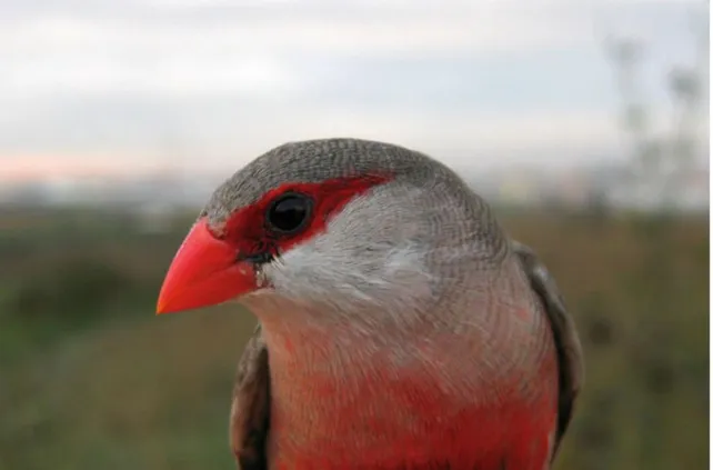
The common waxbill (Figure 1) is a bird within the family Estrildidae native to sub-Saharan Africa which has known successful invasions in the Iberian Peninsula as well as various regions of Brazil and several tropical islands. The common waxbill is a small, colourful, granivorous finch. They are opportunistic breeders that take advantage of favourable conditions for reproduction, resulting in having a variable time of breeding throughout the year. They are not migratory but highly gregarious and have nests scattered in loose colonies. Because of their small but colourful appearance, they have been a subject of pet trade around the world ever since the nineteenth century. When the independence wars in Angola and Mozambique began in the 1960s and Portuguese colonists started migrating from these colonies to Portugal, so began the invasion of the common waxbill. It is uncertain if these events are related to each other. Following these early introductions, the waxbill population in Portugal kept increasing and several other introduction events might have happened along the way where waxbills were introduced in areas further away from the existing distribution at the time. The first waxbill habitats were mainly connected to water. By the 1990s common waxbills had completely colonized the Portuguese coast. Currently common waxbills have invaded a large part of the Iberian Peninsula consisting of Portugal and several regions in Spain (Cardoso et al. 2018). Records of common waxbills in Brazil go as far as the 1870s. Since then, the common waxbill is present in most of the east coast of Brazil (Da Silva et al. 2018). In addition to these two major non-native regions, the common waxbill has also successfully colonized several tropical islands around the globe including Cape Verde, Canary Island, Oahu and parts of the Seychelles archipelago (Stiels et al. 2011).

Because the common waxbill is such a successful tropical invasive bird, it is also a promising species to get a better understanding of the dynamics of a biological invasion (Stiels et al. 2011). The mechanistic bio-energetics model Niche Mapper is a relative new and ever-changing model that has already successfully predicted several species distributions; but it has also faced criticism, i.e. it relies too much on the reliability of the available data. The time and resources needed to sample the needed parameters of a large amount of individuals are often too costly. As a result only a few individuals are used to calibrate the mechanistic model. However, with the amount of evidence proving the existence of local adaptations, this limited data sample might result in an underestimation of the full fundamental niche of a species (Peterson et al. 2015). Therefore, this thesis focusses on the common waxbill as a case study to test the ability of the mechanistic model Niche Mapper to accurately predict the current distribution of the common waxbill.

(9)

9

2. Objectives

Aforementioned, the objective of this thesis is to evaluate the ability of Niche Mapper to accurately predict the current distribution of the common waxbill in Europe, Africa and South-America and thus to evaluate how well the fundamental niche of the common waxbill can explain its distribution in native and non-native regions. For this purpose, this thesis has been split into three sub-objectives. First I will perform a metabolic chamber analysis using Niche Mapper (Sub-objective 1). This will allow me to evaluate the obtained data and model settings. The output of this model will provide me with the expected thermoneutral zone for the common waxbill which I will compare to the acknowledged thermoneutral zones in literature to check how realistic the output is. This subobjective can be considered a model quality control step.

Secondly, I will perform a sensitivity analysis of the different variables that Niche Mapper uses to predict the distribution of the common waxbill (Sub-objective 2). Performing this analysis will enable me to derive which variables have the most impact on the accuracy of the ecophysiological model and thus which traits of the common waxbill influence its fundamental niche the most. A separate analysis will be done for Europe, Africa and South-America.

Finally, upon obtaining a good performing model waxbill, Niche Mapper will be used to perform whole continent predictions (Sub-objective 3). This will result in species distribution maps for Europe, Africa and South-America which I can compare to the real current distribution of the common waxbill. This will make it possible to evaluate the accuracy of the model and the predicted fundamental niche of this invasive bird.

Getting a better understanding of the fundamental niche of invasive species can be of great importance to tackle the spreading of harmful invasive species. Knowing and understanding which traits make a species invasive can help future research on these species and their impact assessments. Another fundamental question in ecology is the degree to which niches are spatially and temporally conserved. Because invasive species frequently experience release from biotic interactions and dispersal barriers in their invaded ranges, they are the perfect model systems to research this topic. With the previously mentioned objectives in mind, this thesis will attempt to shed some light onto these matters.

(10)

10

3. Material and methods

To perform these different analyses as well as to make whole continent predictions, the bio-energetics model Niche Mapper was used. The data used in this model came from different sources: most morphological data was measured by a fellow thesis student Marie Stessens; all other data was obtained from literature from the common waxbill or related species. Normally I would have performed a number of measurements on functional traits on live specimen of common waxbills. For example body temperature would have been measured by the use of cloacal heat cameras, however due to the COVID-19 pandemic the measurements on live specimen were cancelled. All R-scripts used in this thesis were provided by Diederik Strubbe, unless mentioned otherwise, and adjusted for common waxbills.

3.1. Niche Mapper

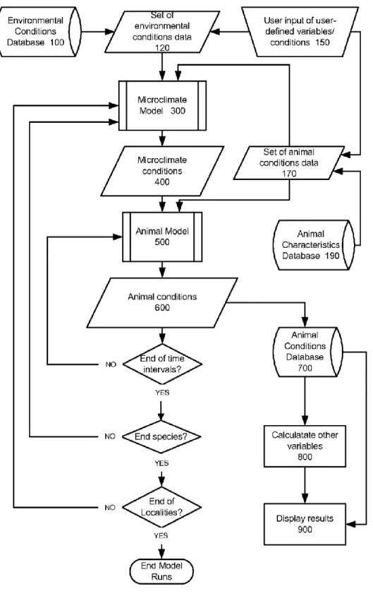
Niche Mapper is a patented mechanistic bio-energetics model that has been developed by Porter and Mitchell (Porter et al. 2001). It calculates the spatial-temporal effects of a variety of environmental conditions on animal individual, population and community dynamics given the animal’s temperature-dependent behaviours, morphology and physiology. In other words, Niche Mapper uses the for a given animal relevant microclimatic data, and combines its behaviour and physical and physiological properties to calculate hourly steady-state body temperature and to find the metabolic rate needed for the animal to maintain these body temperatures (Porter et al. 1973). This results in Niche Mapper being able to model an organism’s fundamental niche with models that are fully parameterized without relying on any information of the species’ distribution as input data and to predict the distribution of the species in a selected region. To obtain these results, Niche Mapper consists of two built-in submodels: a microclimate submodel that returns environmental conditions that are relevant and experienced by the animal; and an animal submodel that uses the output of the microclimate submodel and returns the effect of those environmental conditions on an animal’s metabolic and other variables. These results can then be used for further research, which in this case will be aimed at predicting the geographic distribution of the animal. A simple overview of the method that Niche Mapper uses, is presented in Figure 2.

(11)

11

Figure 2: The conceptual framework of Niche Mapper. (Porter et al. 2001). Sets of environmental and animal data are used as input for the two models. The output of the microclimate submodel is used, in combination with additional animal data, as input for the animal submodel. Finally the output of the animal submodel can be used for further calculations.

(12)

12

3.1.1. Microclimate submodel

The microclimate submodel uses macroclimate data as input such as cloud cover, minimum and maximum daily air temperatures, wind speed and relative humidity, in combination with geographical location, substrate properties and time of the year. The model uses these environmental conditions data to solve a heat-mass balance equation for the above and below ground microclimates over a certain time interval. In addition to this, the model computes several other factors such as solar radiation. Following this, the microclimate submodel combines the results with species-specific information and calculates the climate boundary conditions for an average individual of the species. Finally, the model returns an output of hourly environmental and climate boundary conditions relevant for the given animal for the average day of each month of a single year and the percentage of habitat thermally available to it (Porter et al. 2001, Kearney et al. 2011).

The environmental conditions data needed as input for this model can be a combination from data retrieved from environmental conditions databases and a user-defined set of variables and conditions as depicted in Figure 2. The environmental conditions database that was used for this thesis, is the CRU CL v. 2.0 from the Climate Research Unit from the University of East Anglia. This is a gridded climatology dataset of the monthly means from 1961 to 1990 and was released in 2002.

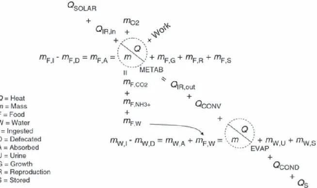
Figure 3: The energy-balance equation used by the animal submodel of Niche Mapper. The diagonal equation is the heat-balance equation where energy is exchanged in the form of heat through different processes of conduction, convection, radiation, evaporation and metabolism. This diagonal equation is intersected by three mass-balance equations. The horizontal mass-balance equation at the metabolism term depicts the mass-balance for dry food; the vertical mass-balance equation at the metabolism term is a representation of the respiratory mass-balance. The last mast-balance equation, at the evaporation term, is a mass-balance equation for water (Kearney et al. 2009).

(13)

13

3.1.2. Animal submodel

The animal submodel consists of two different models, an ectotherm model and an endotherm model. The common waxbill, being a bird, is an endothermic animal, so I used the endotherm animal submodel for further analysis. This submodel uses the microclimate conditions output together with animal characteristics data to calculate animal conditions output. To achieve this, the model uses heat-transfer principles to calculate an animal’s heat in its local microclimate informed by morphological, physiological and behavioural information (Mathewson et al. 2013). The model calculates the desired metabolic rate that will enable an animal to maintain its body temperatures within a tolerable range. This heat-mass balance equation states that the animal’s metabolic heat generation must equal heat transfer through its fur/feathers and the net heat flux with its microenvironment in order to maintain its core body temperature during each hour of the day. A more detailed description of the energy balance equation used by the animal submodel of Niche Mapper is displayed in Figure 3 (Porter et al. 2001, Kearney et al. 2009, Kearney et al. 2011).

Following this, the results of the equation are used to calculate several energetic variables including total discretionary energy and water, temperature dependent activity of the animal, and the total annual activity of the animal. The model then returns an output of these energetic variables together with the solutions from the energy-balance equation, including values such as the metabolic heat generation needed to maintain the animal’s core body temperature. The output for all specified time intervals and locations will then be accumulated in an animal model conditions database to allow for (1) further calculations to analyse spatial and temporal dynamics of the species, and in the case of this thesis, (2) the coupling of GIS based information on climate, topography and vegetation so it can be used to generate a species distribution prediction.

3.1.2.1. Morphological data measurements

The additional animal characteristics data required as input for this submodel have been gathered from various sources and collected in an Excel file where all the required variables were listed. A fellow thesis student, Marie Stessens, measured several morphological traits from 122 different common waxbill specimens that were part of the collections of two different musea, the Royal Belgian Institute for Natural Sciences at Brussels and the Royal Museum for Middle-Africa at Tervuren. These specimen were all common waxbills that originated from their native sub-Saharan range and were kept at these musea. The morphological traits measured included the length, the horizontal and vertical intersections and the feather length and depth of the head, the neck and torso; and the length of the complete body, the tail, tarsus, tibia, legs and beak. Every specimen has been fully measured twice to account for any incorrect measurements. For a more detailed description of how these measurements were executed, I refer to the thesis of Marie Stessens. Using this data I calculated the mean, median and standard deviation across all specimen for further use in the animal submodel.

(14)

14

3.1.2.2. Reflectivity

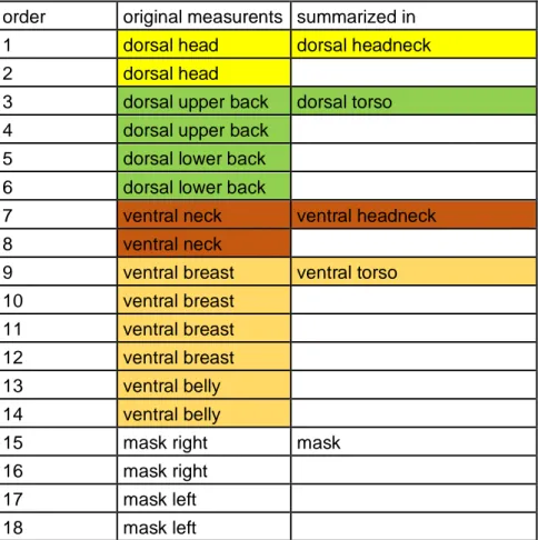
Niche Mapper also requires the input of the dorsal and ventral reflectivity for the head and neck; and the torso. Reflectivity can be a very important trait in the thermoregulation of an animal for it is the deciding factor at how well heat from the sun gets absorbed or reflected. I was able to use a dataset that has been collected by Ananya Agnihotri (Agnihotri 2020). She used this data for a research that focussed on the ability of the common waxbill to respond to environmental stressors in both native and invasive ranges. Ananya measured the reflectivity of 41 different waxbills on 8 different body parts from a wavelength of 299,764nm to 2028,497nm. Because Niche Mapper only needs the reflectivity of the previously mentioned ventral and dorsal body parts, the measurements by Ananya had to be summarized before I was able to use them in Niche Mapper (Table 1). To summarize this data in the four body parts that are required for Niche Mapper, I used an R script based on an R script that Merel Stadt used to calculate the reflectivity of the fur of brown bears (Ursus arctos) (Stadt 2020). First I corrected the data for any negative values and then I adjusted the script to fit reflectivity data of common waxbills collected by Ananya. The output of this script could then be used to calculate the mean and standard deviations of the reflectivity for each required body part across all measured waxbills.

order original measurents summarized in

1 dorsal head dorsal headneck

2 dorsal head

3 dorsal upper back dorsal torso

4 dorsal upper back

5 dorsal lower back

6 dorsal lower back

7 ventral neck ventral headneck

8 ventral neck

9 ventral breast ventral torso

10 ventral breast

11 ventral breast

12 ventral breast

13 ventral belly

14 ventral belly

15 mask right mask

16 mask right

17 mask left

18 mask left

Table 1: The eight body parts that were measured by Ananya for reflectivity. All measured body parts have at least one duplicate. All measurements, except those for the mask, were then summarized within a mean with the help of R and used as input for Niche Mapper (Agnihotri 2020).

(15)

15

3.1.2.3. Literature study

As previously said, normally I would have taken measurements of various functional traits on live specimen, but due to the COVID-19 pandemic and the resulting lockdown, these measurements were cancelled. Instead all the remaining data that was required for Niche Mapper was obtained by a literature study. I collected an extensive and diverse amount of data from various sources. When I had multiple sources for the same variable, I compared them to obtain the most realistic value possible. Unfortunately, for some important variables, no data of the common waxbill existed in available literature. As a substitute, I had to obtain the value from two related species, namely the black-rumped waxbill (Estrilda troglodytes) and the orange-cheeked waxbill (Estrilda melpoda). These values were then tested and adjusted accordingly with the metabolic chamber analysis, described below, to build a model average common waxbill that can be used in further analysis.

3.2. Metabolic chamber analysis

The first analysis I executed, was the metabolic chamber analysis. The purpose of this analysis is to check whether the inputted data creates a realistic common waxbill by returning a thermoneutral zone, which I compare to the thermoneutral zone found in literature. All data that has previously been collected, was summarized in an Excel file with two sheets. The first sheet contains all allometric variables (AlomVar) and the second sheet contains all endothermic variables (Endo) that are used by Niche Mapper. These variables were transferred to two R scripts, one for the allometric variables and one for the endothermic variables. When ran, these R scripts return respectively an alomvars.dat and an endo.dat file, which are ready to use for Niche Mapper. Next, Niche Mapper uses these two files, together with files that describe the microclimate, to solve the energy-balance equation and returns hourly outputs for an average day per month as described above. Finally I used a third R script to filter this data and to display the thermoneutral zone for a common waxbill with the inputted values.

Hereafter I could use the resulting thermoneutral zone to compare to the thermoneutral zone of common waxbills found in literature. Unfortunately, no existing records of the thermoneutral zone of common waxbills were available in literature so I had to compare it to the thermoneutral zone of the two related species that have been previously mentioned, the orange-cheeked waxbill and the black-rumped waxbill.

Next I varied several important variables that affect the thermoneutral zone of the common waxbill, such as the BMR, body mass and core body temperature. Because of this I was able to see how the thermoneutral zone of the waxbill reacted to the adjustment of some of these key parameters. This allowed me to correct and verify several variables that I found in literature, especially the variables which originated from the related species instead of the common waxbill itself, as well as to verify some of the variables that were measured by Marie or Ananya and transformed by me. Altogether this allowed me to build a model average waxbill that will be used in further analysis for this thesis.

(16)

16

3.3. Sensitivity analysis

The sensitivity analysis is an expansion of the first steps of the metabolic chamber analysis. In short the metabolic chamber analysis gets executed for a random set of values and this is repeated 1000 times resulting in 1000 different sets of results. Afterwards the results of these metabolic chambers were compared to a set of locations where the common waxbill is either present or absent, to determine how well this set of random values fit the real distribution of the waxbill. Finally the 1000 different results were compared to each other to determine which key species traits are the most influential on the distribution of the common waxbill.

3.3.1. Preparing the microclimate data

Before the analysis can start, the microclimate data for the chosen locations has to be prepared for use. These locations are selected from the presence data of the common waxbill from the GBIF database. In addition to this presence data, absence data is also needed to be able to compare the two. However GBIF only provides occurrence data and no real absence data, so pseudo-absences have to be selected. Random selection might produce inaccurate models because the background size from which pseudo-absences are selected, has important ramifications for the performance of SDMs. Pseudo-absences that are too similar in environmental space to that of the occurrences result in spurious predictions; pseudo-absences that are drawn from an exceedingly large area can lead to over simplified predictions with less informative response variables (VanDerWal et al. 2009). To account for this, for every occurrence location, 10 different pseudo-absences were randomly selected in the given continent. These occurrences and pseudo-absences are represented by ‘pixels’ that are 10x10km grids with lat-long coordinates in each continent (Figure 4).

All of this has been done by using an R script that starts with the selection of these locations and further continues with the preparation of the microclimate data. When these locations are specified, the preparation of the microclimate data for each location can start. To prepare this microclimate data, R will simply read several grid maps from the continent that specify the year-round climate for each location on the whole continent. This microclimate data will be linked by R to the locations of the occurrence and the pseudo-absence data to create the necessary microclimate files needed by Niche Mapper for each location. The microclimate data is then ready to use for further analysis.

(17)

17

Figure 4: Example of a selection of occurrence and pseudo-absence data in Europe. Red crosses are occurrences obtained from GBIF, black crosses are pseudo-absences that were randomly selected by R with 10 pseudo-absences for each occurrence.

3.3.2. Model creation

When the microclimate data had been prepared, I could start with the creation of the 1000 different model variations, once again, with the help of R. As previously said, each model had a different set of random values for the traits of interest. These random values were always relatively scaled, based on the original values that had been inputted by me. These original values were those of the model average waxbill that had been created by the metabolic chamber analysis. This resulted in some models for example having a higher basic metabolic rate but a lower reflectivity and others having a higher reflectivity but a lower body temperature. Not every trait was altered in the different models. Only those traits known to affect the homeothermy and thermal neutral zone were used to make different random model variants (Table 2).

.

Traits used for LHS

body mass feather depth feather length

density fat percentage BMR

BMR activity BMR breeding feather diameter

feather density feather reflectivity core body temperature delta core-skin temperature delta inhaled-exhaled temperature

(18)

18

x

Figure 5: A Latin Hypercube in a 2-dimensional space, called a Latin Square, containing 4 samples. Each hyperplane, in this case 1-dimensional rows and columns, only contain one unique sample.

To create these 1000 different random models the Latin Hypercube Sampling method was used. Latin Hypercube Sampling (LHS) is a near-random sampling method developed by Michael McKay (McKay et al. 1979). The method creates a k-dimensional space with k equal to the number of variables of which the random sampling is desired, in this case 14 variables (Table 2). Next, the range of each variable is divided in x equally large intervals with x being the number of desired samples which has to be decided in advance, in this case 1000 samples. Finally x samples will be placed into the k-dimensional space while taking into account that each hyperplane created by the intervals on each variable, may only contain one sample. Each sample is a random point contained in its corresponding interval for each variable. An example of a Latin Hypercube with only two dimensions, called a Latin Square, is shown in Figure 5. A big advantage of this method is that each sample gets selected while taking into account previously selected samples, resulting in the LHS method having a ‘memory’ of all previous samples which ensures that the samples are representative of the real variability.

Once this Latin Hypercube had been created, 1000 different samples were placed within, while satisfying the above mentioned requirements. This resulted in 1000 different model variants of common waxbills, each with different variations of the traits mentioned in Table 2, ready to be used by Niche Mapper.

(19)

19

3.3.3. Model evaluation

With both 1000 different common waxbill models and microclimate data ready for use, Niche Mapper can be run to determine the energy requirement the waxbill needs in each location. However, the energy requirement for the breeding period differs from the non-breeding (survival) period so these two periods are separated and every model was ran, once for each period to atone for that. Similarly to the metabolic chamber analysis, the R-script creates endo.dat and alomvars.dat files for each separate model. Next R calculates the energy requirement needed to breed or to survive in each of the selected locations consisting of the occurrences and pseudo-absences.

Once the energy requirement for both periods in every location of all 1000 modelled waxbills is known, the breeding and survival counterparts of each model can be combined to estimate which locations are suiTable for which model variants. This is done by looking at the metabolic rate needed for the waxbill to maintain its body temperature. Simply put, the colder the ambient temperature gets, the higher the metabolic rate needed for the waxbill to maintain its body temperature and homeothermy. The warmer it gets, the lower the metabolic rate has to be. If a location is so warm that the required metabolic rate in order for the animal to maintain its body temperature and homeothermy is lower than the basal metabolic rate (BMR), the animal will die from overheating for this is an impossible requirement to meet. On the other hand, it has been stated that birds cannot maintain a metabolic rate higher than 4,6 times its BMR for a longer period of time. If the temperature of a location is so cold that the required metabolic rate in order for the waxbill to maintain its body temperature and homeothermy is higher than 4,6 times its BMR, it will die from hypothermia. The field metabolic rate (FMR), i.e. the average metabolic rate an animal produces on an average day, of a common waxbill is stated to be around 2,5 times its BMR. This leaves 2,1 times its BMR as tolerance until the cap of 4,6 times its BMR has been reached and the animal might die from hypothermia. However, during breeding periods the metabolic rate of a waxbill is 4 times its BMR, leaving only 0,6 times its BMR until the cap of 4,6 times its BMR is reached (Lindström et al. 1995, Kearney et al. 2016). These metabolic rates are separately for each location and modelled waxbill. A location will be considered suiTable if the location is not too warm or too cold for the waxbill to survive throughout the year and breed for at least three subsequent months.

Once the suitability of every location is calculated for each model, this fit of locations can be compared to the actual occurrences and pseudo-absences of the locations and the accuracy of every model is computed. This is done by using the True Skill Statistic (TSS), a method for assessing the accuracy of SDMs. It’s an improvement on the widely used kappa statistic by accounting for its criticized dependency on prevalence. It does this using the following formula:

𝑇𝑆𝑆 = 𝑆𝑒𝑛𝑠𝑖𝑡𝑖𝑣𝑖𝑡𝑦 + 𝑆𝑝𝑒𝑐𝑖𝑓𝑖𝑐𝑖𝑡𝑦 − 1

Sensitivity refers to the proportion of correctly predicted presences and specificity to the proportion of correctly predicted absences, or in this case pseudo-absences. The resulting TSS can range anywhere from -1 to +1, where +1 indicates a perfect agreement between the prediction and the reality, and values of zero or less indicating a performance that equals random (Allouche et al. 2006).

(20)

20

The TSS is calculated for each model by using the occurrences and the same amount of pseudo-absences. As previously stated, there might be inaccuracies with the pseudo-pseudo-absences. To account for this, the calculations are repeated 10 times for each model, with different pseudo-absences being selected each time. Finally the mean of these 10 TSS’s will be calculated and assigned to the corresponding model variant.

For the final step of this sensitivity analysis, all models and corresponding TSS are evaluated using Boosted Regression Trees (BRT). BRT is a combination of two algorithms: regression or decision trees and boosting. Decision trees are easily interpreTable tree-based models that do not rely on prior data transformation or elimination of outliers and automatically model interaction effects between predictors. However they are often not as accurate as other statistical methods, such as GLM, and thus have poor predictive performance. BRT overcomes this disadvantage by using the concept of boosting. Boosting improves model accuracy based on the idea that it is easier to find and average many rough rules of thumb, than it is to find a single, highly accurate prediction rule. BRT uses this concept to fit multiple regression trees instead of a single tree. The first tree is the one that maximally reduces the loss of predictive performance. Then a second tree is fitted on the residuals of the first tree, reducing the loss of predictive performance even further. This continues until a linear combination of multiple regression trees is formed. This final BRT model has a predictive performance superior to most traditional modelling methods while keeping the advantages of regression trees (Elith et al. 2008).

By using such BRT machine learning, I was able to determine which key species traits have the most impact on the TSS and accuracy of the model, and to determine the most important key species traits for the distribution of the common waxbill on the modelled continent. This analysis is repeated for the three continents where the common waxbill is present: Europe, Africa and South-America.

3.4. Whole continent predictions

The third analysis that I performed, was the distribution prediction of the common waxbill for all three of the entire continents. This analysis uses the same concept as the first steps of the sensitivity analysis. As opposed to the later, no occurrence and pseudo-absence data is selected and no model variants are created. Instead the variables of the entire model are based on the values of the model average common waxbill created by the metabolic chamber analysis. Subsequently, every pixel, 10x10km grid, of the entire continent is evaluated and marked suiTable for this model average common waxbill if it meets the metabolic rate requirements that have previously been listed. Eventually a map of the continent is created with colour-coded pixels: black for areas that do not meet the metabolic requirements of this common waxbill; and colour for the pixels where the waxbill is able to survive and breed. A colour gradient is created to indicate the amount of energy needed for thermoregulation in each pixel. Finally this map is compared to the known occurrences of the common waxbill and a TSS is created to display the accuracy of the model. This whole analysis is once again performed by an R script and is executed for Europe, Africa and South-America.

(21)

21

4. Results

4.1. Metabolic chamber analysis

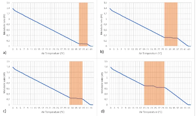
The output of the metabolic chamber analysis resulted in a graph that displays the air temperature in relation to the metabolic rate. From this graph the thermoneutral zone (TNZ) of the common waxbill with the model settings can be derived: increasing the BMR lowered the temperature range of the resulting TNZ of the waxbill; and decreasing the BMR raised the temperature range of the TNZ (Figure 6). Another interesting result is that the range of the TNZ increases with a higher BMR.

Figure 6: The ambient temperature in relation to the metabolic rate for the common waxbill for different BMR values for a waxbill with a body mass of 0,0089kg. The thermoneutral zones of each model variant is marked with an orange box. a) BMR of 10 W/kg, which is a total BMR of 0,089 W. b) BMR of 27 W/kg, total BMR is 0,24 W. c) BMR of 35 W/kg, total BMR is 0,31 W. d) BMR of 75 W/kg total BMR is 0,67 W.

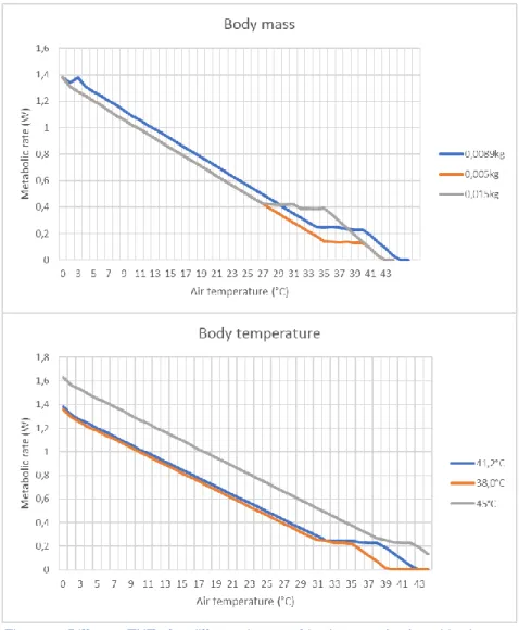
Analogous with the BMR, an increased body mass lowers the temperature range of the TNZ while a decreasing body mass results in a higher TNZ. In contrast, lowering the body temperature of the waxbill returned a lower temperature range for the TNZ, while a higher body temperature returned a higher temperature range for the TNZ. However the metabolic rate from the TNZ stays the same, whereas with other traits it changes accordingly (higher BMR or body mass results in higher metabolic rate for the lower TNZ) (Figure 7). Adjusting the waxbill’s fat percentage does not prompt any significant changes in the TNZ. This analysis was performed for all values that were not directly measured, resulting in a model average common waxbill that was used in the subsequent analyses.

(22)

22

Figure 7: Different TNZs for different inputs of body mass (top) and body temperature (bottom). Not all inputted values are realistic; they were purely used to test the response of the TNZ. The value that is used in the final model is marked in blue.

4.2. Sensitivity analysis

The sensitivity analysis was done separately for all three continents of interest, each with their own unique results. As previously stated in Table 2, the sensitivity analysis was performed for 14 different key species traits that varied across all 1000 different model variants. The output of each analysis consists of the relative importance of each variable of interest, or key species traits, along with the interaction effects between those variables and the TSS of each model variant. The results will be presented in three different sections.

(23)

23

4.2.1. Africa

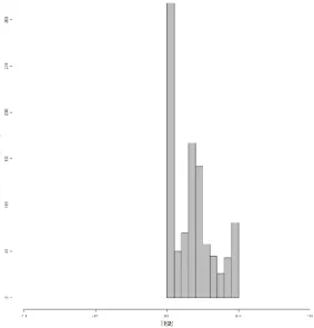
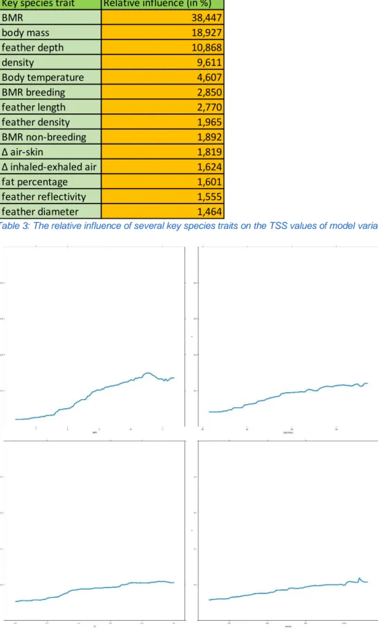
The relative importance of each key species trait for common waxbills in Africa is shown in Table 3. As illustrated the BMR has the highest impact on the TSS of the model variants of waxbills in Africa and can thus be considered the predominant species trait for their distribution on this continent. It is followed by the body mass, the feather depth, the density and finally the body temperature (Figure 8: left). It is clear that the other parameters are less influential on the TSS. None of these model variants were however able to accurately predict the full distribution of the common waxbill in Africa as shown in Figure 8: right. Most model variants had a result that equals random (TSS ≤ 0), as one would expect, but the maximum TSS value reached by these models was only 0,5 suggesting that the most adequate model variants were only able to predict around 75% of the occurrences and absences of the waxbill in Africa.

The relation of the four most impactful variables to the TSS is depicted in Figure 9. A positive correlation between the TSS and the values of these variables can be noticed, however, the TSS has a peak for increasing BMR around 10,5 W/kg. The other values keep increasing but seem to reach an upper limit.

Figure 8: Left: The relative importance of each variable tested in Africa. From top to bottom: BMR: Basic metabolic rate, body.mass: body mass, fd: feather depth, density, Tb: body temperature, BMR.Act.B: BMR during breeding periods, fl: feather length, f.dens: feather density, BMR.Act.M: BMR during non-breeding periods, Tairskin: temperature difference between core body and skin temperature, Texinhaled: temperature difference between inhaled and exhaled air fat.perc: fat percentage, f.refl: feather reflectivity, and f.diam: feather diameter. Right: The frequency distribution of the model variants along with their corresponding TSSs in Africa.

(24)

24

Table 3: The relative influence of several key species traits on the TSS values of model variants in Africa.

Figure 9: The four most impactful key species traits in function of their influence on the TSS in Africa. Top left: BMR in W/kg; top right: body mass in g; bottom left: feather depth in mm; bottom right: density in kg/m³.

Key species trait Relative influence (in %)

BMR 38,447 body mass 18,927 feather depth 10,868 density 9,611 Body temperature 4,607 BMR breeding 2,850 feather length 2,770 feather density 1,965 BMR non-breeding 1,892 Δ air-skin 1,819 Δ inhaled-exhaled air 1,624 fat percentage 1,601 feather reflectivity 1,555 feather diameter 1,464

(25)

25

Finally, the interaction effects between the BMR and several of these variables and the corresponding TSS are shown in Figure 10. Again an optimal TSS value for the BRM is reached after a steady increase around 10,5 W/kg. When accounting for the interaction between BMR and body mass, this optimal TSS value is already reached with a lower BMR if the body mass is high enough, emphasising the importance of the co-operative interaction between BMR and body mass. Additionally, body mass seems to have a more significant effect on the TSS with higher BMR values. To a minor extent, this interaction effect is also visible between BMR and feather depth. However, between BMR and body temperature, or BMR and density, it is practically absent.

Figure 10: The interaction effect of the BMR and one other key species trait in relation to the TSS value. Top left: interaction between BMR and body mass; Top right: interaction between BMR and feather depth; Bottom left: interaction between body temperature and BMR; Bottom right: interaction between BMR and density.

(26)

26

4.2.2. Europe

As is the case with Africa, BMR has the most influence on the TSS scores of the model variants (Figure 11: left). The body mass however, is now considered the sixth most influential variable on the TSS scores compared to the second highest relative importance in Africa. Feather depth also seems have less relative importance in Europe compared to Africa, but body temperature is approximately the same value. The second most influential variable in Europe is the feather length. This in contrast to Africa, where its relative influence was the seventh highest. The feather length in Europe is almost twice as important for the TSS score compared to the body mass in Africa, with scores of 32,4% and 18,9% respectively (Table 4). Another noTable observation is that breeding BMR is almost six time as important than in Africa and all other variables except feather diameter and reflectivity, have less relative importance.

In comparison with the analysis for Africa, the TSS scores of the highest scoring model variants in Europe are able to predict the occurrences and absences more accurately. Several models scored a TSS of 0,8 or higher, indicating a predictive accuracy of about 90% (Figure 11: right). This is remarkable since the morphological measurements that were used for this thesis were all performed on waxbills that originated from several regions in Africa.

The responses of the four most influential variables to the TSS score of the model variants are displayed in Figure 12. BMR, feather length and density increase with increasing TSS scores without reaching an obvious optimum. BMR however only has an observable effect on the TSS at values above 20 W/kg, which is twice as much as the BMR values in Africa.

Figure 11: Left: The relative importance of each variable tested in Europe. From top to bottom: BMR: Basic metabolic rate; fl: feather length; density; Tb: core body temperature; fd: feather depth; body.mass: body mass; f.dens: feather density; Tairskin: temperature difference between core body and skin temperature; f.diam: feather diameter; f.refl: feather reflectivity; fat.perc: fat percentage; BMR.Act.M: BMR during non-breeding periods; Texinhaled: temperature difference between inhaled and exhaled air; BMR.Act.B: BMR during breeding periods. Right: The frequency distribution of the model variants along with their corresponding TSS in Europe.

(27)

27

Table 4: The relative influence of several key species traits on the TSS values of model variants in Europe.

Figure 12: The four most impactful key species traits in relation to their influence on the TSS in Europe. Top left: BMR in W/kg; top right: feather length in mm; bottom left: density in kg/m³; bottom right: core body temperature in °C.

BMR 42,372 feather length 32,403 density 6,743 body temperature 4,353 feather depth 3,632 body mass 2,162 feather density 2,045 Δ air-skin 1,591 feather diameter 1,421 feather reflectivity 1,269 fat percentage 0,682 BMR non-breeding 0,470 Δ inhaled-exhaled air 0,437 BMR breeding 0,419

(28)

28

Because the body mass is of considerably lower relative importance than in Africa, the interaction effect between the body mass and BMR and their influence on the TSS score is much less prominent, although still present at high BMR and body mass values (Figure 13). However, between the BMR and feather length a noticeable interaction is present: a high BMR only equals high TSS scores when the feathers are long enough and vice versa. Combining high values of both variables can already result in TSS scores of almost 0,5, resulting in a model prediction with an accuracy of about 75%. Such an interaction is also present between BMR and density: increasing BMR is more influential on the TSS if the density is high enough. The interaction between BMR and core body temperature suggests that the positive effect of BMR on the TSS score is only present within a certain temperature range, indicating the optimal body temperature. It is noteworthy that this interaction was not noticeable in the results from the Africa analysis.

Figure 13: The interaction effect of the BMR and one other key species trait in relation to the TSS value. Top left: interaction between BMR and body mass; Top right: interaction between BMR and density; Bottom left: interaction between BMR and feather length; Bottom right: interaction between body temperature and BMR.

(29)

29

4.2.3. South-America

Once again the BMR has the largest relative influence on the TSS scores of the model variants (Figure 14: left, Table 5). The value is even higher than in Europe. However, as is the case in Africa, the second most influential variable is the body mass. This is followed by the density, feather length, feather depth and finally the core body temperature as sixth most influential variable. Feather length has a considerable smaller influence on the TSS scores in South-America than in Europe, but a larger influence than in Africa, albeit only 4% larger. Overall, the relative influence of these key species traits is more comparable to the values of Africa than Europe, with the exception of the above mentioned differences.

The TSS frequency distribution of the model variants implies that a considerable amount of model variants resulted in a better than random TSS score (Figure 14: right). More than 25% of all model variants has a TSS score of 0,75 or higher, implying an accuracy of 87,5% or better in the prediction of occurrences and absences. Therefore the model variants of South-America have the highest TSS scores of all three continents.

Figure 15 displays the resulting TSS scores from different values of the four most influential key species traits. The BMR reaches the same value as the BMR in Europe, but the resulting TSS score is much higher than both Europe and Africa. The three other traits displayed, body mass, density and feather length, also reach higher TSS scores than in Europe and Africa. Once again the TSS increases with increasing values for these traits.

Figure 14: Left: The relative importance of each variable tested in South-America. From top to bottom: BMR: Basic metabolic rate; body.mass: body mass; density; fl: feather length; fd: feather depth; Tb: body temperature; BMR.Act.M: BMR during non-breeding periods; B Tairskin: temperature difference between core body and skin temperature; f.refl: feather reflectivity; f.dens: feather density; Texinhaled: temperature difference between inhaled and exhaled air; fat.perc: fat percentage and f.diam: feather diameter; MR.Act.B: BMR during breeding periods. Right: The frequency distribution of the model variants along with their corresponding TSS in South-America.

(30)

30

Table 5: The relative influence of several key species traits on the TSS values of model variants in South-America

Figure 15: The four most impactful key species traits in relation to their influence on the TSS in Africa. Top left: BMR in W/kg; top right: body mass in g; bottom left: density in kg/m³; bottom right: feather length in mm.

BMR 48,966 body mass 16,971 density 10,431 feather length 6,176 feather depth 4,513 body temperature 3,745 BMR non-breeding 1,359 Δ air-skin 1,287 feather reflectivity 1,225 feather density 1,148 Δ inhaled-exhaled air 1,110 fat percentage 1,057 feather diameter 1,044 BMR breeding 0,966

(31)

31

As was the case in Africa, an obvious interaction effect between BMR and body mass is present (Figure 16). The other three compared interactions, BMR with feather depth; density; and core body temperature, also display interaction effects, but they are less prominent. Most influence comes from the BMR on its own and a higher value of the other variables do not necessarily lead to a higher TSS score than the sum of both variables. This indicates that the strongest interaction effects are noticeable in the sensitivity analysis of Europe.

Figure 16: The interaction effect of the BMR and one other key species trait in relation to the TSS value. Top left: interaction between BMR and body mass; Top right: interaction between BMR and feather density; Bottom left: interaction between BMR and density; Bottom right: interaction between body temperature and BMR.

(32)

32

4.3. Whole continent predictions

Using the model average common waxbill evaluated in the metabolic chamber analysis, distribution predictions for Africa, Europe and South-America were made. These predictions were executed separately from the sensitivity analysis. While some model variants reached very high TSS scores, this does not guarantee a high accuracy and TSS for the predictions made using the common waxbill that was evaluated in the metabolic chamber analysis.

The output of this analysis is a map for each given continent displaying the possible distribution of the common waxbill according to the specific model settings. The pixels are colour-coded: black represents locations that are not suiTable for this specific common waxbill; coloured pixels represent locations which are. The different colours depict the amount of energy that the waxbill would have to invest in thermoregulation to remain in homeothermy in that specific location . The distribution prediction for Africa, the native continent of the common waxbill, shows a spread throughout the entire continent with the exception of regions in northern Africa and South-Africa (Figure 17). The prediction suggests that the common waxbill would need to invest the least amount of energy in thermoregulation in the sub-Saharan tropical rainforests. However, the actual distribution of the common waxbill shows how they seem to avoid these rainforests and settle for the green-coloured pixels, i.e. which are locations where an intermediate amount of energy is required for thermoregulation, and even some blue pixels, i.e. locations with high energy-requirements. While the model predicts that South-Africa is outside of the metabolic range of the common waxbill, in reality, South-Africa houses some of the largest common waxbill populations in the world.

A different observation can be made for Europe (Figure 18). Here Niche Mapper predicts that the entire continent is outside of the metabolic range of this model common waxbill. Even the regions in Portugal and Spain, that have been colonised by the common waxbill in the past century, are considered unsuiTable.

Finally, the predictions for South-America have comparable results to Africa (Figure 19). The tropical rainforests of Brazil are depicted by red-coloured pixels, suggesting that common waxbills in these locations would require the least amount of energy for thermoregulation. Yet in reality, most common waxbills seem to be located on locations depicted by green and even blue-coded pixels, which are locations where the common waxbill would need to invest more energy into their thermoregulation, leaving less energy for other processes.

(33)

33

Figure 17: Species distribution predicted in Africa by Niche Mapper, using the resulting values from the common waxbill from the metabolic chamber analysis as input. Black pixels indicate locations that are predicted to be outside of the metabolic range of the waxbill. Coloured locations lie within this range, the colour gradient indicates the amount of energy the common waxbill has to invest in thermoregulation to remain in homeothermy (depicted as megajoule/year). Triangles indicate populations of the common waxbill that were obtained from GBIF.

(34)

34

Figure 18: Species distribution predicted in Europe by Niche Mapper, using the resulting values from the common waxbill from the metabolic chamber analysis as input. Black pixels indicate locations that are predicted to be outside of the metabolic range of the waxbill. No coloured pixels are present in this prediction. Triangles indicate populations of the common waxbill that were obtained from GBIF.

(35)

35

Figure 19: Species distribution predicted in South-America by Niche Mapper, using the resulting values from the common waxbill from the metabolic chamber analysis as input. Black pixels indicate locations that are predicted to be outside of the metabolic range of the waxbill. Coloured locations lie within this range, the colour gradient indicates the amount of energy the common waxbill has to invest in thermoregulation to remain in homeothermy (depicted as megajoule/year). Triangles indicate populations of the common waxbill that were obtained from GBIF.