Identification and handling of
uncertainties in dietary exposure
assessment
Report 320103004/2009
RIVM Report 320103004/2009
Identification and handling of uncertainties in dietary
exposure assessment
H.J. van Ooijen
H. van der Voet, Biometris, WUR M.I. Bakker
Contact: M.I. Bakker
Centre for Substances and Integrated Risk Assessment martine.bakker@rivm.nl
This investigation has been performed by order and for the account of the Dutch Food and Consumer Product Safety Authority, within the framework of the project Modelling humane dietary exposure to contaminants
© RIVM 2009
Parts of this publication may be reproduced, provided acknowledgement is given to the 'National Institute for Public Health and the Environment', along with the title and year of publication.
Abstract
Identification and handling of uncertainties in dietary exposure assessment
The RIVM and the RIKILT-Institute of Food Safety estimate the intake of chemical substances via food at the population level. The method presently used for dietary exposure assessments should be adapted to allow more insight into the extent of the uncertainties in such exposure estimates. The quantification of uncertainties is in line with international scientific endeavors that are currently being carried out in the field of uncertainty analysis of exposure assessment. In addition to the quantification of uncertainties, it is important to consider the expected impact of the (remaining) non-quantified uncertainties on the dietary exposure estimate. These are the conclusions drawn by the RIVM and Wageningen University and Research Centre (WUR) based on a study carried out by these institutes by order of the Dutch Food and Consumer Product Safety Authority (VWA). This report contains a proposal for adapting the current software program (Monte Carlo Risk Assessment) as well as two examples that illustrate the use of the Guideline of the European Food Safety Authority for describing non-quantified uncertainties.
An analysis of the uncertainties in an exposure assessment is necessary to enable a proper interpretation of the assessment results. Uncertainty analysis can also highlight those factors that are the major sources of uncertainty in the dietary exposure assessment. By decreasing (the impact of) the most important sources of uncertainties (e.g. by collecting additional data), (future) exposure assessments can be improved.
The software program currently used by the RIVM and the RIKILT is able to perform a limited quantitative uncertainty analysis. This program could be expanded in a relatively simple manner by including the quantification of a number of other sources of uncertainty.
Rapport in het kort
Identificeren van en omgaan met onzekerheden in de beoordeling van blootstelling aan stoffen via voeding
Het RIVM en het RIKILT-Instituut voor Voedselveiligheid schatten hoeveel chemische stoffen mensen via voeding binnenkrijgen. De huidige methode zou meer inzicht moeten kunnen geven in de mate waarin deze blootstellingsschattingen onzekerheden bevatten. Het kwantificeren van onzekerheden sluit aan bij de internationale wetenschappelijke activiteiten die momenteel op het gebied van onzekerheidsanalyse van blootstellingsschattingen gaande zijn. Naast het kwantificeren van meer onzekerheden moet de invloed van de (overgebleven) niet-gekwantificeerde onzekerheden op de blootstellingsschatting worden beschouwd.
Deze conclusies blijken uit onderzoek van het RIVM en Wageningen Universiteit en Researchcentrum (WUR), dat in opdracht van de Voedsel en Waren Autoriteit (VWA) is uitgevoerd. In dit rapport wordt een voorstel gedaan om de huidige software (Monte Carlo Risk Assessment) aan te passen. Tevens wordt aan de hand van twee recente praktijkvoorbeelden geschetst hoe de richtlijn van de Europese Voedselveiligheidsautoriteit (EFSA) toegepast kan worden voor het beschrijven van
niet-gekwantificeerde onzekerheden.
Een onzekerheidsanalyse is nodig om de resultaten van blootstellingsschattingen van stoffen beter op hun waarde te kunnen schatten. Bovendien kan een onzekerheidsanalyse aanwijzen welke bronnen van onzekerheid een belangrijke bijdrage leveren aan de totale onzekerheid van de blootstellingsschatting. Door vervolgens gericht de belangrijkste onzekerheden te verminderen (door bijvoorbeeld additionele gegevens te verzamelen) kunnen (toekomstige) schattingen worden verbeterd.
Momenteel kan de software van het RIVM en het RIKILT een beperkte kwantitatieve
onzekerheidsanalyse van een blootstellingsschatting uitvoeren. De methode zou relatief eenvoudig kunnen worden uitgebreid met het kwantificeren van een aantal andere bronnen van onzekerheid. Trefwoorden: onzekerheidsanalyse, blootstellingsschatting, innameberekening, blootstelling, MCRA
Contents
Summary 9
1 Introduction 11
2 Uncertainty in dietary exposure assessment 13
2.1 Model for dietary exposure assessment 13
2.2 Uncertainty and variability in dietary exposure assessment 15
2.2.1 Uncertainty and variability 15
2.2.2 Sources of uncertainty in dietary exposure assessment 15
3 Model uncertainty 19
3.1 Conceptual model boundaries 19
3.2 Statistical model dependencies 19
3.3 Conceptual and statistical model assumptions 20
3.4 Conceptual model detail 21
3.5 Conceptual model extrapolation 21
3.6 Conceptual and statistical model implementation 21
3.7 Using other conceptual models 21
4 Model input uncertainty 23
4.1 Uncertainty in consumption data 23
4.1.1 Bias in consumption data 23
4.1.2 Lack of precision in consumption data 24
4.2 Uncertainty in concentration data 26
4.2.1 Sampling uncertainty 26
4.2.2 Uncertainty due to composition of samples 28
4.2.3 Analytical uncertainty 29
4.3 Uncertainty in linking consumption and concentration data 30
4.3.1 Different types of linking 30
4.3.2 Processing factors 31
5 Analysis of uncertainty in dietary exposure assessment 33
5.1 Analysis of model uncertainty 33
5.1.1 Quantitative analysis of model uncertainty 33
5.1.2 Qualitative analysis of model uncertainty 33
5.2 Analysis of model input uncertainty 34
5.2.1 Quantified model input uncertainty 34
5.2.2 Qualified model input uncertainty 34
5.3 Examples of qualitative uncertainty analysis 35
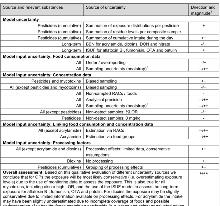
5.3.1 Example 1: Long-term dietary intake of dioxins 35 5.3.2 Example 2: Dietary intake of various compounds by children 37
6 Discussion 41
7 Conclusions 45
References 47
Appendix 1 Validation of new versions of MCRA 51
Summary
In the Netherlands, dietary exposure assessments of chemical substances are performed for the Food and Consumer Product Safety Authority at the RIKILT Institute of Food Safety and at the National Institute for Public Health and the Environment. These two institutes use the program Monte Carlo Risk Assessment (MCRA) to derive the dietary intake of substances (De Boer and Van der Voet, 2007). In the MCRA program exposure is estimated in a probabilistic way.
There are a large number of sources of uncertainty in exposure assessment (e.g. chemical analysis of food products, biased sampling, food consumption surveys, modelling usual intake) and the
uncertainties can be large. An analysis of these uncertainties is required to enable a proper
interpretation of the outcome of an exposure assessment. Hence, a thorough uncertainty analysis can aid policy makers in taking decisions with respect to dietary exposure to substances.
Exposure assessors should strive to assess the relative importance of all sources of uncertainty and at least quantify the most important sources. The current release of the MCRA program incorporates options to quantitatively estimate some types of uncertainty. These are the sampling uncertainties of consumption data and concentration data and specified uncertainty concerning processing factors. In addition, at present some forms of model uncertainty can be investigated by running alternative models or model variants and comparing the outputs. However, the use of the latter is limited as the true model outcome is not known.
It is recommended to extend the uncertainty analysis in the MCRA program. This can be done by taking more sources of uncertainty in dietary exposure assessment into account. Examples for which this can be carried out are the number and size of meal portions, the uncertainty in analytical
measurements, the composition of the sample (unit variability) and ingredient percentages in recipes. In addition, subjective expert opinions and probabilistic elicitation techniques may be appropriate to quantify the up-till-now non-quantified uncertainties.
Whereas a fully quantitative uncertainty analysis is the most informative analysis, this cannot be reached due to the high costs. Therefore, qualitative analysis of some of the uncertainties will remain and therefore it is important to consider them. They should be listed, along with the estimated magnitude and direction, preferably according to the tabular format as is proposed by the European Food Safety Authority. Two examples are given in this report. More experience with procedures for qualitative uncertainty assessment is needed.
The quantification of uncertainties is in line with international scientific endeavors (by e.g. EFSA and WHO) that are currently being carried out in the field of uncertainty analysis of exposure assessment.
1 Introduction
There are a large number of sources of uncertainty in exposure assessment of chemical substances (e.g. chemical analysis of food products, food consumption surveys, modelling usual intake) and the uncertainties can be large. The World Health Organization states that uncertainty analysis should be an integral part of exposure assessment (WHO, 2008). A thorough uncertainty analysis allows a proper interpretation of the exposure assessment results and therefore it can aid policy makers in taking decisions on dietary exposure to substances. As uncertainty analysis is not a purpose in itself, but serves as a tool, the level of detail in the uncertainty analysis should be in line with the needs of the exposure assessment (driven by the risk assessment, i.e. what question is addressed?) and the availability of data necessary to execute the uncertainty analysis.
Uncertainty analysis in exposure and risk assessment has received increasing attention in the last decade. Since 2001, NUSAP, a framework in which quantitative and qualitative uncertainty analysis for environmental risk assessment is described, has been developed (www.nusap.net). NUSAP is a notational system which enables the different sorts of uncertainty in quantitative information to be displayed in a standardized way. In this way uncertainties in the information, whether it is a process feature or a numerical detail, become clear.
In 2006, the scientific committee of the European Food Safety Authority (EFSA) prepared a guidance document related to uncertainties in dietary exposure assessments (EFSA, 2006). An example of how this can be applied was provided in an EFSA opinion on acute dietary exposure assessment of pesticide residues in fruit and vegetables (EFSA, 2007). Additionally, in 2008, a guidance document was presented by a working group of the International Program on Chemical Safety (WHO, 2008).
The framework proposed by EFSA and WHO consists of a progression from lower, simpler uncertainty analyses to higher, more complex tiers of uncertainty analyses. Tier 0 consists of a point estimate that is derived with conservative assumptions (and default values). With Tier 1 the point estimate is more refined and an indicative range for the associated uncertainty is given. Tier 2 introduces multiple point estimates based on different combinations of assumptions; the uncertainty in the point estimates can still not be quantified. The last tier encompasses a probabilistic dietary exposure assessment (or semi-probabilistic as the ADI is deterministic). If ADIs are made semi-probabilistic (as for example is done in Integrated Probabilistic Risk Assessment, Van der Voet and Slob 2007; Bokkers et al., 2009) Tier 4 is possible.
In the Netherlands, dietary exposure assessments of substances are performed for the Food and Consumer Product Safety Authority at the RIKILT Institute of Food Safety and the National Institute for Public Health and the Environment (RIVM, Centre of Substances and Integrated Risk Assessment). Subsequent risk assessments of those substances are performed at the RIVM. The RIVM and the RIKILT use the program Monte Carlo Risk Assessment (MCRA) to derive the dietary intake of substances (De Boer and Van der Voet, 2007). In the MCRA program exposure is estimated in a probabilistic way. The current release of the MCRA program incorporates possibilities to estimate some sources of uncertainty, but there are more sources of uncertainty in dietary exposure assessment that may be taken into account. As the confidence intervals reported by MCRA only encompass a limited number of sources of uncertainty, they can give an incomplete impression of (un)certainty. The EFSA and WHO guidances on uncertainty analysis in dietary exposure give the first methodical guidance to uncertainty analysis in dietary exposure assessment. The present document elaborates on these two reports and specifically addresses the uncertainty analysis of the dietary exposure assessment performed with MCRA. The goal of the present report is to make an inventory of sources of uncertainty
of a population’s exposure to a certain contaminant through food intake. Furthermore it is demonstrated how these sources are presently quantified in the computation of dietary exposure with MCRA.
Subsequently, the implementation of additional methods for the quantification of uncertainty in the MCRA program is proposed.
As the present report addresses exposure assessment using MCRA, this document does not address the uncertainty analysis of deterministic exposure (Tier 0, 1 and 2) assessments. In addition this report does not consider the uncertainty in the hazard characterization nor in the assessment of risks associated with the intake of a particular compound.
In chapter 2 of the present report background information is given about the method of dietary exposure assessment and the sources of uncertainty therein. Two important types of uncertainty, namely model uncertainty and model input uncertainty are described in chapter 3 and 4, respectively. Chapter 5 addresses the current methods of uncertainty analyses in dietary exposure assessment. In the final chapters proposals (chapter 6) and conclusions (chapter 7) on the optimal handling of
2 Uncertainty in dietary exposure assessment
This chapter gives an introduction into dietary exposure assessment as it is performed with MCRA and the sources of uncertainty therein.
2.1 Model for dietary exposure assessment
Conceptual model
The aim of dietary exposure assessment as it is performed at the Centre for Substances and Integrated Risk Assessment (SIR) at the RIVM and the RIKILT – Institute of Food Safety is to obtain the variability in intakes of the population. The first step of the assessment is to obtain data on food consumption by the relevant population and on concentration data of the compound of interest in the consumed foods (Figure 1). Next, it is necessary to link the concentration data with the consumed food products, as the information on the food products which is available in both data sets does not always correspond with each other (e.g. French fries are consumed, but only concentration data of potatoes are available). For this linking process, information on recipes is used. In addition, the processing (peeling, washing, cooking etc.) of food products is taken into account in this step. The final step consists of the multiplication of the consumption and concentration data, and summation over the consumed products on one day of one individual (= a person day), to obtain the dietary intake of this person day. This procedure is repeated for many person days.
consumption data concentration data recipes processing factors
Figure 1.
MCRA
- linking consumption data with concentration data (using recipes and processing factors)
- calculation of intake on a person day as ∑(consumption x concentration) - repetition of calculation of intake for many person days
- additional statistical modelling
Dietary intake distribution
Figure 1. Conceptual model of dietary exposure assessment. Three steps can be distinguished: acquiring consumption data and concentration data, the linking of concentration and consumption data and subsequently the estimation of dietary intake with MCRA, including additional statistical modelling.
In the final step of the assessment, additional statistical modelling is used for different purposes (see below). The steps mentioned above, including the statistical modelling, together form the conceptual model of the dietary intake assessment. This conceptual model is implemented in the computer program Monte Carlo Risk Assessment (MCRA, De Boer and Van der Voet, 2007; De Boer et al., submitted). For this program the food consumption data and concentration data are the two main input datasets. Two other databases, a recipe database and a database with processing factors are used to link the two main input datasets1.
Statistical models for acute and chronic dietary exposure assessment
For assessing acute exposure MCRA derives the intake of the compound on a large number of days randomly chosen from the set of person-days in the food consumption survey. The program accomplishes this by linking the individual’s consumed products to sampled concentrations for this product. So, for each person day (one day of the survey for an individual) the total intake of a
compound per kg body weight of this individual is derived by multiplying the consumed amount with the concentration of the product. By performing many iterations (drawing many person days), a dietary intake distribution (many person days for many individuals) is obtained.
For substances that are present in concentrations that exert chronic toxic effects, the distribution of long-term (usual) intakes (per kg body weight) can also be derived with MCRA. Long-term (usual) intake is defined as the average intake of an individual over an unspecified longer time period. Instead of drawing concentrations from a concentration distribution as is done in the acute exposure
assessment, the average concentration in the consumed food is used to derive the intake. This is done because the average concentration is considered the best representation of the concentration
‘encountered’ by an individual in the long-term.
A very simple method is considering the distribution of observed individual mean intakes (OIM method). However, for chronic exposure assessment a translation is often judged necessary from the short-term survey to the long-term. In the Dutch national food consumption survey, the available consumption data consist of two independent 24-h dietary recalls (or records) per individual. As a consequence, the estimated mean consumption over the available days per individual may suffer from a large sampling error and the corresponding distribution of means over individuals obtained with the OIM-method may be too wide in comparison to the distribution of true usual intakes. For that reason, statistical modelling is used to estimate the long-term (usual) intake using the intake on the (two) survey days. Statistical models that are available for this are for example the Iowa State University model for Foods (ISUF) (Nusser et al., 1996; Dodd et al., 2006) and the Betabinomial-normal (BBN) model (Slob 2006; De Boer et al., submitted). These models take the intake frequency into account, i.e. they model that for some compounds the intake does not take place every day, but only on a fraction of days. The OIM, ISUF and BBN models are implemented in MCRA.
The present chapter addresses the sources of uncertainty in dietary exposure assessment. In the
following chapters the uncertainty emerging in the model as a whole (model uncertainty, chapter 3) and in the parameters and datasets used in the different steps (model input uncertainty, chapter 4) will be discussed.
1Other inputs can be the percentage of a crop that was treated with a compound and the unit variability factor (see also section 4.2.2)
2.2 Uncertainty and variability in dietary exposure assessment
2.2.1 Uncertainty and variability
Data needed to perform a (dietary) exposure assessment usually do not have precise, single values; they contain uncertainty and variability. Variability is an intrinsic property of a parameter and is inherent to the system being modelled, whereas uncertainty represents ignorance or partial lack of knowledge and is thus dependent on the current state of knowledge. As the quality and quantity of the data improves, the uncertainty about their true value decreases (see section 2.2.2), whereas the variability will not decrease or increase with better or more data. There are several options to handle variability and uncertainty in dietary exposure. These are:
1. Only variability is quantified. The estimated exposure is a best estimate of variation in exposure; the resulting distribution can be used to estimate the exposure for different percentiles of the population but provides no confidence intervals.
2. Variability and uncertainty are quantified but not kept separated. The estimated exposure distribution can be used to set uncertainty limits on the exposure for a randomly chosen individual, but it gives no correct estimate of the population distribution itself, and therefore does not allow proper estimates of percentiles.
3. Variability and uncertainty are quantified separately. The output represents the exposure estimates for different percentiles of the population (variability), together with confidence intervals (uncertainty).
The use of option 1 is discouraged as it gives no impression of (un)certainty. Option 2 is also
discouraged when reporting on risks for the population is the issue. Therefore, for high tier assessments as carried out in MCRA, option 3 is preferred.
2.2.2
Sources of uncertainty in dietary exposure assessment
Sources of uncertainty in exposure assessment can be roughly classified in three categories as indicated by the WHO harmonization project on uncertainty in exposure assessment (WHO, 2008). These three broad categories of uncertainty are scenario uncertainty, model uncertainty and parameter uncertainty.
• Scenario uncertainty: uncertainty in specifying a scenario that represents the use (e.g. consumption) of the product.
• Model uncertainty: uncertainty in the capability of the conceptual and statistical models to represent the scenario; gaps in scientific knowledge can hamper an adequate capture of the correct causal relations or correlations between inputs of the model (e.g. the relation between consumption frequency and consumption amount).
• Parameter uncertainty: uncertainty in the (input) data (e.g. concentration, consumption and processing data)
Classification of uncertainty using these three broad categories is not as strict as it may seem; in practice the uncertainty may arise from overlapping categories. For example, a calibrated model parameter fitted against a data set suffers from uncertainty in measurement (parameter uncertainty) as well as incompleteness of the model (model uncertainty).
The categorization used in the present report is a further specification of (and partially an amendment on) the classification proposed in WHO (2008): we prefer the term ‘purpose uncertainties’ to ‘scenario uncertainties’ because scenarios may also concern different input data. In addition, we prefer ‘model input uncertainty’ to ‘parameter uncertainty’ because in probabilistic modelling of dietary exposure
there are both data sets (concentration data, consumption data) and parameters (e.g. fraction of ingredient in a food) as model inputs, and for an uncertainty analysis these inputs should be treated similarly. On the other hand, we feel that bias and precision of model inputs should often be treated in different ways, so we have separate categories ‘model input bias uncertainty’ and ‘model input precision uncertainty’.
On this we base a main classification of uncertainties for probabilistic dietary exposure assessment: 1. Uncertainties regarding the purpose of the exposure assessment
Probabilistic dietary exposure assessment is performed using a statistical model to derive one or more specific outputs (e.g. a percentile of the exposure distribution or the probability to exceed a limit value). For an uncertainty analysis to be performed it is essential that these output variable(s) are clearly defined. For example: Is the assessment to be made for a population of persons or for person days? Is the interest in p95, or p99 or any other percentage? Is the interest in the cumulative effect of a group of compounds, or of a specific compound? Should metabolites be included? Is it internal or external exposure? For which population do we want an answer (time, space, age classes), e.g. Dutch children 1-6 years in 2008 or Dutch children 1-6 years 1997/98? Should exposure be modelled as a function of covariates (e.g. age) or overall?
Uncertainties regarding the purpose of the exposure assessment are not further discussed in this document as such uncertainties should be eliminated in collaboration between risk assessors and risk managers before the exposure assessment is started.
2. Model uncertainties
Different models may be chosen (at different levels of the intake assessment). Conceptual models may be different either in structure (e.g. estimation of dietary intake by multiplication of consumption and concentration vs. chemical analysis of 24 h duplicate diets2, different statistical models for the derivation of usual intakes) and/or in level of detail (which foods are coded for consumption and concentration data? Is processing included?).
To clarify how model uncertainties are different from model input uncertainties (category 3 below) we can envisage an ideal data situation, where all (conceptual) model inputs would be exactly known, say because enormously large error-free databases on each relevant aspect (consumption, concentration, linking, processing, etcetera) were available. There would then still be remaining uncertainties due to the choice of a specific statistical model (e.g. results of ISUF and BBN models could be different due to different assumptions in both models). Thus the category ‘model uncertainty’ contains all remaining uncertainties when optimal data would be available.
Model uncertainties can be partly assessed in sensitivity analyses3 using alternative models; in the software there could be alternative options to investigate this. For example, in MCRA one can choose either the ISUF or the BBN model. Note that the comparison of two unvalidated models could be misleading: Even if the models agree, they may be subject to the same biases, or they may give the same results for different reasons. However, comparing two models is the best option when there are no validation data. It may be helpful in identifying errors in the structure of the model, the computer code
2 24 h duplicate diet: A duplicate sample of all food which has been eaten by an individual during a 24 h period is collected and pooled into one composite sample in which compounds are measured.
3 In a sensitivity analysis the susceptibility of a model is determined by detecting changes in the output when the value of an input parameter is changed (or when an alternative model is being used). A sensitivity analysis is not equal to an uncertainty analysis: the latter consists of an estimation of the total uncertainty of the model output, based on an evaluation of the input uncertainties. However, partitioning the total uncertainty into contributions from several inputs is commonly called sensitivity analysis.
or the model inputs (See Cullen and Frey, 1999). Chapter 3 will describe model uncertainty in dietary intake assessment in more detail.
3. Uncertainties in model inputs
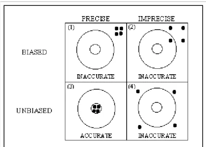
These can be divided in the bias and lack of precision of model inputs. 3a. Bias
Model inputs may be biased (i.e. they have a tendency towards eing either too high or too low) (see Figure 2) and therefore not represent the true state of nature. Of course, if such biases are known quantitatively, then a correction procedure can be included in the model, and only the uncertainty of this correction would remain (as a contribution to category 3b, see below). But generally objective quantitative information about the size of the bias is not known. (An exception may be for analytical measurements, for which the use of internal standards and quality control may quantify the bias). When bias cannot objectively be quantified, it should be assessed by expert judgment.
3b. Lack of precision
Model inputs may have a limited precision (Figure 2). Datasets may be small, and parameter values may be obtained from limited information. Note that the set of parameters may include correction factors introduced in the model to avoid biases. For example, a factor for ‘percentage non-treated’ may be used to avoid that all non-detect pesticide concentrations are replaced by small values such as the limit of detection (or half the value of the limit of detection as often is performed). Lack-of-precision uncertainties are in principle open to data-based quantification in software, but expert judgment may also be needed. For example, several studies on the same processing factor may give different results, and the variation between the results may be used as a quantification of the uncertainty. In other cases, only one estimate for a processing factor may be available necessitating the use of an expert opinion on its uncertainty.
Our classification separates the uncertainties which can in principle be quantified in the software, at least partially (category 2 by having multiple options, category 3b in the estimation itself), from uncertainties that should be addressed before performing the exposure assessment (categories 1 and 3a). Note that quantitative corrections for the analytical measurements need to be performed before the MCRA-program is run.
Figure 2. An example of bias and precision. Four gun shots at a target can be inaccurate due to e.g. a biased gun and/or an imprecise shooter.
3 Model uncertainty
Here we give a list of model uncertainties as mentioned in WHO (2008), and provide some specific points of attention for dietary exposure assessment as we perform it by the four steps mentioned above and using the MCRA program.
3.1 Conceptual model boundaries
Results of dietary intake assessments using MCRA are uncertain if MCRA is applied for situations other than dietary acute or chronic exposure assessment. Cumulative exposure assessment can be done by prior application of ‘relative potency factors’ (RPFs), such as toxic equivalency factors (TEFs) for dioxins, to the concentrations of individual compounds followed by an MCRA analysis of the weighted sum. Nevertheless, this is only possible if the compounds have the same mechanism of action and parallel dose-response curves. The determination of the RPFs is based on experimental data and therefore contains uncertainty. Because with the current version of MCRA the weighing has to be done outside the program, these uncertainties cannot be accounted for. In addition, working with the
weighed sum in probabilistic calculations amounts to drawing from only one distribution of concentrations (for the index compound), and therefore drawing for example a high value from this distribution amounts to drawing a similarly high value for all individual chemicals. Clearly, this absolute correlation among chemicals in a sample is unrealistic and leads to uncertainty about the estimated exposure distribution.
3.2 Statistical model dependencies
In dietary exposure assessment in which consumption is multiplied with concentrations, independence of consumption of foods and concentration in those foods is assumed, which is considered a reasonable assumption in general. However, there may be exceptions, such as avoidance of allergenic compounds by allergic consumers, or avoidance of food which shows the signs of decay connected with the presence of certain compounds.
In chronic risk assessment, there is an uncertainty in the estimation of intakes by MCRA because possible dependencies between intake frequency and intake amount are not accounted for. In acute risk assessment, concentrations of a compound in multiple foods are assumed to be independent, which is uncertain to be true under all circumstances. Processing factors are modelled as fixed values or by distributions. In the case of distributions no dependencies are included in the model.
3.3 Conceptual and statistical model assumptions
In the conceptual model it is assumed that the intake can be estimated by multiplication of consumed amount of a food and the concentration measured in this (or sometimes a similar) food, using recipes and processing factors to estimate the concentrations in food products that are not analyzed themselves. In acute risk assessment not many additional model assumptions are made: the exposure assessment relies on a direct Monte Carlo resampling of individuals with their associated body weight and consumption pattern, and measured concentrations for each of the consumed foods. Uncertainty may arise from specific parts of the model. First, when concentration data are made in composite samples, a model is needed to estimate concentrations in single units. Uncertainty arises because there are various options for this model and of course none of these may capture the true situation.
In chronic exposure assessment more assumptions have to be made, which may not represent reality well. First of all, for the estimation of the long-term (usual) intake, the assumption is that a
transformation to a scale can be made where the intake can be represented as an additive model. This means that the intake is represented by the sum of a general mean intake and two deviation terms: the individual deviation and the person-day deviation. The former addresses that the mean intake of an individual’s intake over a large number of days deviates from the overall mean intake in the population, whereas the latter represents that the intake on any day for an individual deviates from that individual’s mean intake.
For chronic exposure assessments the BBN and ISUF models are implemented in MCRA. The BBN model assumes that the usual intake amounts are normally distributed after a logarithmic or power data transformation (i.e. . y=log(x) or y=xλ, respectively). The choice of transformation is a source of uncertainty in itself. Normality may not be achieved, so the assumption of normality may not be always correct. The ISUF model is designed to generate normality at a transformed scale by the use of an additional spline4 transformation (so here an assumption is not made). Nevertheless, the assumption in
ISUF is that the additive model mentioned above is still correct on this highly artificial
spline-transformed scale5. Preliminary results of studies with real and simulated data seem to suggest that the assumption may not always hold (De Boer et al., submitted; Slob et al., submitted), leading to a large uncertainty.
The dependency of the chronic exposure on covariates (e.g. age, sex) is modelled. There are several possibilities to model the dependency on continuous covariables such as age, for example polynomial6,
exponential or spline functions. There is uncertainty concerning the choice of the appropriate function for modelling the dependency on covariables, but it is generally considered low.
In the final step of the dietary exposure assessment the short-term intake is derived by the
multiplication of the concentrations and the consumption amounts of the consumed foods on one day. MCRA performs this by drawing an individual from the survey, combining his or her consumption
4spline: a spline is a special function defined piecewise by polynomials
5 this is necessary because the statistical analysis on this normal scale used for deriving the usual intake distribution relies on this additive model
6 a polynomial is an expression constructed from variables and constants, using the operations of addition, subtraction, multiplication, and constant non-negative whole number exponents. For example, x2 − 4x + 7 is a polynomial, but x2 − 4/x + 7x3/2 is not, because its second term involves division by the variable x and also because its third term contains an exponent that is not a whole number
with a drawn concentration from the concentration dataset (NB in a chronic assessment: average concentration) and sums the intakes via the different approaches on one day.
3.4 Conceptual model detail
Many aspects of the real world are not represented in the model, although in principle this could be done if sufficient data are available. Most importantly, in MCRA the level of detail used in the coding of food products can be increased indefinitely, but in practice it is not useful to extend this list to a level of detail where no data are available. For example, MCRA can distinguish brands of food with their corresponding market shares, and in a future release a model for brand loyalty will be included, to give a more accurate intake estimate. Nevertheless, this is only useful when concentrations of substances are different in different brands and when information on market shares and brand loyalty is available.
3.5 Conceptual model extrapolation
Uncertainty arises when a model is used outside the intended domain of application. For example, MCRA is intended for the estimation of external exposure (intake rather than uptake), and cannot predict internal exposure or blood concentration-time curves.
3.6 Conceptual and statistical model implementation
Although new versions of MCRA are validated against the previous version (see for an example Appendix 1), implementation of models in software always runs the risk of programming errors that only become apparent for certain scenarios and input combinations. Apart from programming errors some of the algorithms7 need a certain data quality and quantity. The algorithms may give erroneous
results when a model is fitted to too few or scattered data. For example, for the estimation of the usual intake the variation between days is needed. It is questionable if data on just 10 individuals having a positive intake on 2 days is sufficient to derive the variation. Such uncertainties may be examined by comparing results of MCRA to results of alternative programs or by performing simulation studies (see section 5.1.1).
3.7 Using other conceptual models
In the previous sections we considered a specific conceptual model and the uncertainty connected with that model. Alternatively, another conceptual model can be applied to assess the uncertainty of the conceptual model as implemented in MCRA. For example it is possible to assess dietary exposure in a different way than by combining regular consumption data with concentration data by performing a
duplicate diet study. In a duplicate diet study ‘real’ exposures of a number of participants are measured, whereas in dietary exposure assessment as described in chapter 2 the exposure of a number of
4 Model input uncertainty
In this chapter we consider the uncertainties related to inputs of the conceptual model. The model inputs are subdivided in consumption data (section 4.1), concentration data (section 4.2) and the linking of consumption with concentration data, including processing factors (section 4.3).
4.1 Uncertainty in consumption data
In this section we discuss how consumption data may give a biased assessment of true consumption (section 4.1.1) and how the amount of consumption data may give rise to a lack of precision about knowing the true food consumption (section 4.1.2).
4.1.1
Bias in consumption data
Method of data collection
There are several methods to record the consumption: dietary recall, dietary record, household budget surveys, et cetera. In dietary exposure assessments in the Netherlands, data of the Dutch National Food Consumption Survey are often used.
The third Dutch National Food Consumption Survey (DNFCS 3) is the most recent population-wide food consumption survey. It is a dietary record study that contains the consumption data of
6250 individuals for two consecutive days (Kistemaker et al., 1998). Note that DNFCS 3 is already ten years old. The data in DNFCS 3 may provide a biased estimate of the current consumption pattern. At present, a new population-wide survey is performed, which will be finished in 2010.
In 2005 and 2006 a consumption survey on young children (2-6 y) has been performed. In this survey food consumption data was also collected using the dietary record method. In this approach caretakers of the children completed a detailed diary about all the foods and drinks consumed on two non-consecutive days by 1279 children (Ocké et al., 2008).
The methodology of dietary records is regarded as the best available method to assess individual dietary eating habits. The obtained data are suitable to assess the acute and chronic dietary exposure to compounds. However, this method may underestimate consumption levels due to high participation burden (Biró et al., 2002).
Another disadvantage of food consumption surveys is that habitual eating patterns may be influenced or changed due to the recording process. As a consequence the estimation of the exposure may be biased. For example, due to the unhealthy image of crisps and French fries the consumption of these foods may be underreported resulting in an underestimation of acrylamide intake. On the other hand, foods that are known to be healthy like fruits and vegetables may be eaten more on recording days than in practice, which may result in an overestimation of the intake of pesticides. The extent in which eating habits are changed due to the recording process and consequently the effect on the derived exposure levels is unknown.
In the DNFCS Young Children the data was checked on over- and underreporting by deriving the energy needed for basic metabolism. This showed that there was no discrepancy between energy demand and reported intake in the children’s survey (Ocké et al., 2008).
There may also be alternative ways to gather consumption data. In the DNFCS the consumption is studied using dietary records or recalls. With these methods, participants evaluate their consumption on one day at a time, specifying the portions. In addition to the record or recall, participants are asked to complete food frequency questionnaires (FFQs) in which the frequency of the consumption of specific products is inquired (e.g. every day, once a week, once per month). In this method, emphasis is put on the consumption behaviour in the long run and not on the precise portion on one day. A dietary exposure assessment based on FFQs may therefore be an interesting different conceptual model for Step 1, especially when the assessment considers foods that are not frequently consumed. However, FFQs will not comprise the whole range of consumed foods, as this is unfeasible. The use of FFQs as an alternative for dietary records or recalls will therefore only be functional for cases in which a limited number of products, present in the FFQ, is relevant for the dietary intake of a substance (e.g. fish, relevant for the intake of e.g. mercury).
Another method to obtain information on food consumption is the household budget survey. This survey provides descriptions of an individual household’s total consumption and expenditures in relation to characteristics of the household (e.g. size, composition, income), its accommodation and durable goods. However, the detail of a household budget survey considering food consumption is too low for a realistic dietary intake assessment
.
Population
The participants of the DNFCSs are randomly chosen from (internet) panels from marketing research agencies. However, these panels are likely not representative for the Dutch population as a whole. The bias of the population of participants may be reduced by using weighing factors, giving a larger weight to individuals belonging to social-economic classes which are underrepresented in the survey. The use of weighing factors is not implemented in MCRA yet, but this is planned. It may be possible to address uncertainties about these weighting factors if such information is available.
People who do not speak Dutch are excluded from the surveys. Since this cannot be overcome by using weighing factors, the estimated consumption pattern is biased.
Survey days
To obtain an unbiased consumption data set regarding sampling moment DNFCS 3 and DNFCS-Young Children are evenly spread over the whole year and the days of the week. Holidays and anniversaries are excluded from the data. Note that this may cause bias, especially if one is interested in foods that are often consumed on these days.
4.1.2
Lack of precision in consumption data
Number of consumers in the survey
Consumption surveys only sample a small part of the relevant population. For example, in DNFCS 3 there are 6250 persons to represent a Dutch population of around 16 million. The fact that the sample has only a limited number of persons results in a sampling uncertainty of the dietary exposure. Generally, the sampling uncertainty is considered to be small in comparison to other uncertainties. In the case of long-term exposure assessment the limited number of days per person that are sampled leads to an additional imprecision in these data: With only two days per person, as in the DNFCS, the observed individual means will have a large sampling error (this is the reason to apply statistical modelling to translate the observed distribution to a better estimate of usual intake). Moreover, the consumption on two consecutive days (as in DNFCS 3) is probably not independent: on the second
survey day participants may consume left-overs from the first day. A dietary survey on two non-consecutive days, as in DNFCS-Young Children, will therefore give a better representation of reality. Consumption frequency
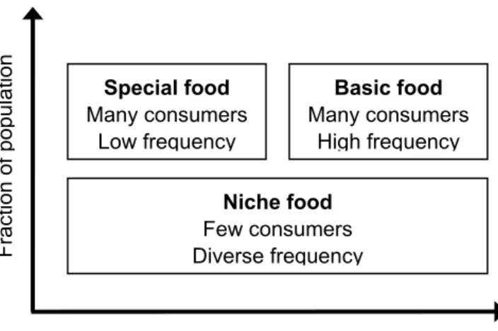
Uncertainty in the food products’ consumption may also reside in the percentage of consumers with a positive intake and the frequency of consumption per consumer. Basic food is consumed by a large fraction of the population frequently and the information regarding the intake frequency included in the DNFCS are relatively accurate (Figure 3). Another category of products are the special foods, which are consumed by a large fraction of the population at low frequency, such as wine. As the food consumption surveys consist of a small number of days, many of the more specific foods will not be consumed in these two days and are reported as ‘zeroes’. Hence, the precision of the information on intake frequency of these special foods is less than for basic foods (Figure 3). A third food category contains the so-called niche foods, which are consumed by a very small fraction of the population. Examples are oyster, eel, couscous. The intake frequency of these foods is too low to perform a reliable intake estimation with DNFCS data (see also section 3.6 on model implementation).
Although there may be large uncertainties regarding the consumption frequencies of single foods, it should be noted that the ISUF and BBN models in MCRA use the intake across foods (total diet approach), so that uncertainties about single foods may be less relevant. It is unknown in how far the lack of information on specific foods is relevant for the percentiles of the total intake distribution. Probably this will vary from case to case. The long-term risk models estimate the percentage of ‘incidental zeroes’(persondays without relevant consumption) and the ISUF model also estimates the percentage of non-consumers (persons never eating the relevant foods). However, the uncertainty about consumption frequencies is not well-known.
Niche food Few consumers Diverse frequency Special food Many consumers Low frequency Basic food Many consumers High frequency Fra ction of po pulation Frequency of consumption
Figure 3. Three categories of food products, classified by fraction of population and frequency of consumption. (Adopted from Bakker, 2002).
Consumption amounts
There is also uncertainty on the reported amounts of consumed foods. Whereas this uncertainty is currently usually not quantified, work is ongoing to make this more explicit (e.g. in the EU-project of Food Consumption Validation (http://www.efcoval.eu)). For example, using the EPIC-SOFT software
interviewed consumers are guided through several choices, and several quantification methods can be used, such as choosing from a series of photos showing different amounts of a certain food or
specifying a proportion of a household measure (e.g. half a bowl of yoghurt). In general, there will be uncertainty about standard portion sizes and about the number of these standard portions consumed.
4.2 Uncertainty in concentration data
The second step of a dietary exposure assessment consists of the estimation of the compound’s concentration in food. The available monitoring data need to be collected or a sampling program needs to be designed to obtain a representative data set on concentrations of the compound in foods consumed by the general population.
Sources of uncertainty in the determination are the sampling uncertainty, uncertainty due to combining samples before, and the analytical error. Both can have components of bias and of lack of precision.
4.2.1
Sampling uncertainty
One of the uncertainties in the sampling of foods is: how well do the sampled foods reflect the foods consumed by the population? This depends on the variability of the concentration in the foods and the bias. When the variability of the concentration is low, a high precision can be reached with a small sample size, whereas for a large variation the sample size needs to be large to yield a precise
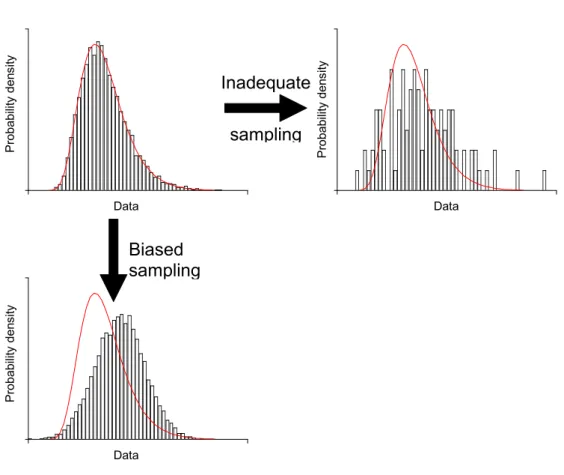
concentration distribution. An insufficient number of samples will result in an imprecise definition of the concentration distribution (see upper right panel of Figure 4). In theory, it is possible to reduce the uncertainty associated with sampling uncertainty by taking more samples. However in practice this is very expensive.
Besides the sample size, it is important to sample the whole range of occurring concentrations. Targeted (or biased) sampling of food products, whether on purpose or not, will result in a distribution weighted by the higher concentrations (see lower left panel of Figure 4 and Boon et al., 2008). As a result the dietary intake, both acute and chronic, will be overestimated. The bias of the sampling procedure is hard to quantify a posteriori. The uncertainty associated with the sampling procedure could possibly be assessed by expert judgement.
Inadequate
sam
pling
Biased
sam
pling
Data Pr ob ab ilit y d en si ty P robabilit y den sit y P robabilit y den sit y Data DataFigure 4. A graphical representation of imprecision and bias of concentration data due to a poor sampling strategy. The true, but unknown probability distribution of the concentration data are represented by a line, which is identical in each figure. The distribution of the measured concentration data is indicated by bars. The upper left panel indicates a precise and unbiased sampling of the
concentration data.
Two different sampling strategies to obtain concentration data are currently used: a monitoring strategy to assess whether concentrations in food products are compliant with legal limits (for e.g. pesticides, mycotoxins) and a sample strategy which aims to derive concentration data for dietary exposure assessment. The latter strategy can be sub-divided in sampling single foods (as is performed for e.g. acrylamide, see Boon et al., in preparation) and sampling of composite food groups or units (as is done for e.g. brominated flame retardants, Bakker et al., 2008). To analyse the uncertainty of the different sampling strategies, one would need to perform more than one ‘sampling strategy’ for one compound. E.g. compare sampling of single and composite foods, or samples purchased from the supermarket with monitoring data from the Food and Consumer Product Safety Authority. However, as chemical analysis of foods is expensive, applying multiple sampling strategies to assess the concentration uncertainty is mostly not feasible.
Limited set of food products sampled
The concentration of the compound is only measured in a limited set of food products. The choice which products are incorporated in the measurements is made by experts. The experts, sometimes supported by previous studies or pilot studies, select products that are known to contain high
concentrations of the contaminant and/or are a large source of possible intake. The food products that are not selected are assumed to contain no (high) contamination. This assumption introduces an uncertainty which is very difficult to quantify.
Age and timeframe of dataset
For dietary exposure assessments a recently obtained concentration dataset is preferred over an (out)dated one. This is especially true for foods which have varying concentrations of compounds in products over the years (e.g. dioxins). Furthermore, the time period in which the samples are collected may be relevant. For example, the formation of mycotoxins on food products is dependent on weather conditions and concentrations of these compounds vary from year to year. To estimate the long-term exposure, an (unbiased) average concentration is needed which reflects this long-term. Therefore, it is recommended to use samples from a range of years.
4.2.2
Uncertainty due to composition of samples
Samples of multiple food units
In most dietary intake assessments, samples are pooled, i.e. they consist of more than one food product ‘unit’ (more than one apple, one carton of milk etc). Using these so-called composite samples instead of individual samples introduces uncertainty because several units are taken together in one sample (and the concentration of one unit is not known). The variation in concentrations between composite samples is lower than the variation in the concentrations between the individual samples.
There is a difference in the application of composite samples between acute and chronic dietary intake assessment. This is caused by the fact that for acute intake assessment the whole distribution of concentrations is taken into account, while for chronic intake assessment the average concentration is sufficient to determine the long-term (or usual) intake distribution.
For example, an high concentration of a given pesticide on a batch of apples is diluted with low concentrations in other batches of apples. In acute risk assessment, the interest is in the total variation. So, to account for the variation among the apples a procedure is needed to ‘decompose’ the composite-sample concentrations to values to be expected for single units. In traditional deterministic exposure assessment a so-called (default) variability factor is used to compute a possible value for the acute dietary intake. The variability factor is defined as the 97.5th percentile divided by the mean of the concentration distribution of single unit concentrations. But since this distribution is not known for composite samples, a default value is used for the variability factor (often 3 or 7). In probabilistic assessment of acute risk (in MCRA) one of several distributions (beta, lognormal, Bernoulli) can be chosen to represent unit variability. Given variability factors, and specifications of the number of units in a composite sample and of the unit weights, are used to define parameters for these unit variability distributions (see De Boer and Van der Voet (2007) for details). All required inputs to derive the variability distribution can be uncertain, and therefore can contribute to the total uncertainty in the outputs of dietary exposure assessment.
In case of a chronic dietary intake assessment, modelling of unit variability is not used, as the average concentration is used in the estimation of the intake distribution.
Samples of multiple food products.
In chronic dietary intake assessments, to reduce costs, occasionally composite samples composed of multiple different food products are collected in order to measure the concentration of a whole group of products at once. In this case, information on the variation between the concentrations in the different products is lost.
For example, in the intake assessment of dioxins, several types of beef (meat loaf, roast beef, among others) are combined into one sample (beef), according to the proportions in which these products are consumed in the food consumption survey. The resulting concentration is an average concentration in beef (expressed per g fat). This value is then used to compute concentrations in individual beef products, using the fat concentration of these products (for example: concentration in meat loaf (per g
product) = concentration in composite beef sample (per g fat) × fat fraction of meat loaf (g fat/g product).
The assumption made here is that the (lipophilic) dioxins are all in the fat fraction of the food products. However, this assumption was never validated and therefore is a source of uncertainty.
4.2.3
Analytical uncertainty
Inter/intralaboratory variation
A second step in the determination of the food product’s concentration is the chemical analysis of the substance. The analytical reproducibility variance represents the uncertainty associated with the imprecise sample preparation and analytical method in the sample’s compound concentration value. The sample preparation and analysis of the samples vary among laboratories and it is uncertain if a lab (and if yes, which lab) determined the true value. The variation introduced should be specified by means of the interlaboratory measurement uncertainty. In addition to that, laboratories often report an intralaboratory uncertainty (which is in general smaller than the interlaboratory uncertainty). The inter/intralaboratory variation should be incorporated in the uncertainty analysis of dietary exposure assessment. Laboratories under accreditation schemes are obliged to have a measurement uncertainty estimate for their reported analytical results (ISO 17025). If still no information regarding the (inter/intra)laboratory variation is available a generally accepted empirical model to estimate the interlaboratory variation is the Horwitz curve (Horwitz and Albert, 2006; Thompson, 2007). The Horwitz curve depicts an empirical relationship between the relative standard deviation of reproducibility (RSDR) and the concentration given by:
, (1)
1 0.5log10( ) 0.5 / log 2(10) 0.15
2 C 2 2
R
RSD = − = C− ≈ C−
where C is the concentration in mass fraction (g/g). The curve is more or less independent on analyte, matrix, method and time of publication for concentrations ranging from 10 pg/g to 0.1 g/g (Thompson 2007).
Reporting limits
At relative low levels analytical measurements become less precise. The limit of quantification (LOQ) is often defined as the level where the precision becomes less than a certain value, e.g. RSDR < 30 %.
The limit of detection (LOD) is the lowest concentration of a compound that can be reliably
distinguished from the absence of that compound (commonly when the peak is 3 times the background noise).
In practice, laboratories frequently suppress the reporting of quantitative values below a certain limit value, which has no clear status, and instead they only report results as ‘less-than’ or non-detect. Such a limit is simply called the limit of reporting (LOR). Instead of just reporting the number of samples < LOR, for dietary exposure assessments it would be helpful if analytical laboratories would report as many quantitative results as possible, with an indication of the increased measurement uncertainty for samples <LOD or < LOQ. This would reduce the uncertainty in the concentration data.
In dietary exposure assessments, values below LOR are often substituted by zero, 0.5×LOR and/or LOR. The two extreme scenarios (zero and LOR) give an idea of the variation between the best-case and worst-case scenarios. Another way to deal with non-detects is to model the distribution of the samples below LOR based on the concentration distribution above LOR. Several methods have been used: parametric (distribution-based) methods like the maximum likelihood estimation (MLE) and non-parametric methods like the Kaplan-Meier method (see for an evaluation of these methods Hewett and Ganser, 2007; Antweiler and Taylor, 2008). In dietary exposure assessment of e.g. pesticides it may be necessary to model the data as a mixture of true zeroes and a lognormal distribution of positive
concentrations, which is partly unobserved due to censoring of values below LOR (Van der Voet and Paulo, 2004; Paulo et al., 2005).
In 2008 the European Food Safety Authority established the Working Group on Left-Censored Data to investigate the use of different methods to handle non-detects. This Working Group will report their findings in the summer of 2009. In addition, a statistical method to handle non-detects will be implemented in MCRA by the end of 2009.
4.3 Uncertainty in linking consumption and concentration data
The concentration and consumption data need to be combined in order to calculate the dietary intake. However, the information available in both data sets does not always correspond with each other (e.g. concentrations of a substance are available in wheat, but this is consumed as bread and pasta). As a result, the measured concentrations often need to be manually linked to the consumed products, and this is a source of uncertainty (section 4.3.1). As concentrations are often measured in raw agricultural commodities a further source of uncertainty concerns the specification of processing factors which relate concentrations in food-as-consumed to concentrations in food-as-measured (section 4.3.2).
4.3.1
Different types of linking
The concentration and consumption data need to be combined in order to estimate the dietary intake. However, the information available in both data sets does not always correspond with each other. As a result, the measured concentrations often need to be manually linked to the consumed products. Several linking types can be distinguished:
1. direct link between measured and consumed product (e.g. measurement in milk, consumed product milk);
2. link between measured product and a similar consumed product (e.g. measurement in milk, consumed product chocolate milk);
3. link between measured product group (e.g. in case of composite samples) and consumed product of this group (e.g. measurement in beef, consumed product: roast beef);
4. link between measured product and ingredients of consumed product (e.g. measurements in wheat and apples, consumed product apple pie). If the concentration is available in the individual ingredients of the consumed food product, these concentrations together with the weighted fraction of the ingredients can be combined to estimate the concentration in the consumed food product (e.g. apple pie is divided in milk (5.8 %), eggs (12.1 %), wheat (14.5 %), apple (58.1 %) and sugar (10.7 %). The conversion model for primary agricultural products, CPAP (Van Dooren et al., 1995) contains weighed fractions of raw agricultural commodities (RACs) for all foods consumed in the DNFCS;
Link type 1 contains the smallest uncertainty. The uncertainty in link types 2 and 3 depends on the similarity of the consumed product with the measured product (group). Note that the level of detail of information about the food products is often higher in the food consumption survey than in the concentration data. In link type 4 the uncertainty depends on the variation of the composition of the product and the number of ingredients (uncertainty increases with the number of ingredients). The current version of MCRA has an elaborate system to link food codes (see De Boer and Van der Voet 2007 for details), but there is no quantification of uncertainty in the weight fractions. For example, using CPAP, foods as eaten are converted to a weighed fraction of a certain ingredient per food. Weighed fractions very likely vary, so there is uncertainty whether the correct fraction is used.
In general, consumption data contain more detail than the concentration data. Whereas the DNFCS provides detailed information on the consumed foods (e.g. raw and cooked vegetables have different food codes, for beef there are more than 20 different food codes varying from meatballs to steak), the information about the analysed foods is often limited to a crude food category (e.g. pulses, beef). If the concentration data would be more detailed, the uncertainty in the linking process would be reduced. The linking of consumed food products to measured ones is a ‘subjective’ process. This means that different experts will make different links, and therefore the exposure assessments will likely have different outcomes. To assess the uncertainty in the linking process it is recommended to use different ways of linking and see how it affects the result. Note that, as the true result is unknown, it is unclear which way of linking is the best, but at least the sensitivity to this factor is being shown.
For example, in Boon et al. (in prep.) concentration data of aflatoxin B1 were available for a number of
different nuts (e.g. walnuts, pistachio nuts, almonds, cashew nuts), whereas concentrations for peanuts were not. In the linking process consumed peanuts were linked to a concentration that was the
(weighed) average of all nuts. However, the pistachio nuts had higher concentrations (about a factor of 10) than the other nuts. So, linking the peanuts to the pistachios would have resulted in a higher exposure, while linking the peanuts to e.g. almonds would have resulted in a lower exposure. It may not be known if one of the nuts can be regarded as surrogate, and if so, which one is the best
‘surrogate’ for peanut. However, it is recommended to study the effect on the exposure of the different ways a concentration can be assigned to peanut.
4.3.2
Processing factors
Almost all contaminants’ levels are influenced by food processing. In food processing, the absolute amount of the compound is changed. For example cooking, frying, washing, and other processing can reduce the content of the contaminant in the product. In some rare cases food processing can increase the amount, e.g. when fungi or yeast are producing toxins during storage. Amounts are often measured in raw agricultural products. Hence, the influence of processing needs to be taken into account by using food processing factors, obtained from literature. The data regarding food processing factors are generally scarce and if available often highly variable; this introduces an uncertainty in the concentration data.
In MCRA processing effects can be accounted for in two ways:
1. In the simplest possibility fixed values are given to represent the change in concentration for certain combinations of food and processing.
2. In a more elaborate model it is recognised that processing effects may be variable. For example, apples may be washed differently on different occasions, and consequently the concentration of residue may be diminished more in some occasions and less in other occasions. In MCRA a statistical distribution can be specified to describe this variability(see Appendix 2).
In MCRA the uncertainty about the processing factors is modelled by introducing uncertainty distributions for either the fixed processing factor of for parameters of the variability distribution described above (see Appendix 2 and Van der Voet et al. (2009) for a more detailed discussion of these uncertainties).
5 Analysis of uncertainty in dietary exposure
assessment
Uncertainty analysis of dietary exposure assessment will always reveal two categories of uncertainty: Uncertainties that are quantified and those that are not quantified but qualified. The analysis of statistical model uncertainty (quantified and qualified) will be described in section 5.1, while section 5.2 addresses quantified and qualified model input uncertainty. Examples of qualitative uncertainty analysis of two recent dietary exposure assessments are given in section 5.3
5.1 Analysis of model uncertainty
5.1.1
Quantitative analysis of model uncertainty
The long-term intake is derived using a statistical model. In MCRA, three statistical models (OIM, BBN and ISUF) are implemented. By applying multiple models the model uncertainty is addressed (See for examples Waijers et al., 2004; De Mul et al., 2005). In an appropriate statistical framework to account for the model unceertainty the outcomes of different models may be averaged if there is no science-based preference for one model (Hoeting et al., 1999), but this requires additional modelling tools and is not common practice. As mentioned earlier, one should not present similar outcomes of two unvalidated models as the true result only because they are similar.
When a statistical model has been chosen for a dietary exposure assessment, within this model different options can be chosen. The user should statistically test whether the intake is dependent on age and/or sex. Other decisions to be taken are the type of transformation of consumed amounts (logarithmic or power), whether or not a spline fit is performed on the intake amount in ISUF, and whether the covariable sex or age is fit with a spline or a polynomial in BBN. To analyze the uncertainty of the chosen model options within the selected statistical model, it is recommended to study the sensitivity of the model by varying the different options and evaluating the results.
5.1.2
Qualitative analysis of model uncertainty
Quantification of model uncertainty is not always feasible as it is not always correct to use different models for each model used in the assessment. For example, if the intake distribution is multi-modal, BBN cannot transform this to normality and therefore should be used. In those cases model uncertainty can only be described in a qualitative way, for example according to the guideline prepared by the EFSA (2006). EFSA proposed to identify and score the sources of uncertainty on an ordinal scale (low, medium and high and direction represented by - and +). In section 5.3 two examples of uncertainty assessment using this format are given. In these examples some model uncertainties are included.