NATIONAL INSTITUTE OF PUBLIC HEALTH AND ENVIRONMENTAL PROTECTION BILTHOVEN. THE NETHERLANDS
Report nr 719101005
Incorporation of biomagnification In procedures for environmental risk assessment and standard setting.
R. Luttik (editor), Th.P. Traas and J. de Greef October 1992
Chapter responsability:
Chapter 1 R.Luttik and Th.P.Traas Chapter 2 R.Luttik and Th.P.Traas Chapter 3 Th.P.Traas and J.de Greef Chapter 4 R.Luttik and Th.P.Traas
This research was carried out on behalf of the Directorate General for Environmental
Protectton. Directorate for Chemicals, Safety and Radiatwn Protection, in the frame of project nr 719101 "Ecorouting".
Mailing List
1 • 10 Directoraat-Generaal Milieubeheer, Directie Stoffen, Veiligheid en Straling 11 Directeur-generaal Milieubeheer, Ir.M.E.E.Enthoven
. 12 Plv. Directeur-generaal Milieubeheer, Dr.ir.B.CJ.Zoeteman 13 Plv. Directeur-generaal Milieubeheer, Mr.G.J.R.Wotters 14 Piv. Directeur-generaal Milieubeheer, Drs.P.E. de Jongh 15 - 23 Begeleidingsgroep onderzoek Ecorouting, d.t.v. Drs.R.Luttik 24 - 33 Begeleidingsgroep onderzoek Ecorendement, d.t.v Drs.TH.P.Traas
34 - 43 Onderzoeks-begeleldingsgroep Integrale Normstelling, d.t.v. Dr.J.H.M. de Bruijn 44 Dr.C.W.M.Bodar (Gezondheidsraad)
45 Dr.J.W.Everts (Dienst Getijdewat eren)
46 Dr.B.van Hattum (Instituut voor Milieuvraagstukken) 47 Dr.G.P.Hekstra (Directoraat-Generaal Milieubeheer) 48 Dr.W. Ma (Instituut voor Bos en Natuuronderzoek)
49 Prof.Dr.N.M.van Straalen (Vakgroep Oecologie & Oecotoxtcologie, VU Amsterdam) 50 Drs.W.L.M.Tamis (Centnjm voor Milieukunde Rijksuniversiteit Leiden)
51 Dr.J.Vegter (Toetsingscommissie Bodem)
52 Depot van Nederlandse publikaties en Nederlandse bibliografie 53 Directie RIVM
54 Sectordirecteur Stoffen en Risico's, Dr.lr.G.de Mik
55 Sectordirecteur Milieuonderzoek, Prof.Dr.lr.C.van den Akker 56 Sectordirecteur Toekomstverkenning, Ir.F.Langeweg
57 Hoofd Adviescentrum Toxicologie, Mw.Drs.A.G.A.C.Knaap 58 Hoofd Laboratorium voor Ecotoxicologle, Prof.Dr.H.A.M.de Knjijf
59 Hoofd Laboratorium voor Water en Drinkwateronderzoek, Ir.B.A.Bannink 60 Hoofd Bijzondere Afdeling Immunobiologie, Prof.Dr.A.D.M.E. Osterhaus 61 Hoofd Laboratorium voor Bodem en Grondwateronderzoek, Ir.L.H.M.Kohsiek 62 Hoofd Laboratorium voor Afvalstoffen en Emissies, Ir.A.H.M.Bresser
63 Hoofd Lat>oratorium voor Luchtonderzoek, Dr.R.M.van Aalst 64 Hoofd Centrum voor Wiskundige Methoden, Drs.A.van der Giessen 65 Hoofd Lat)oralorium voor Toxicologie, Dr.W.H.Könemann
66 Hoofd Voorlichting en Public Relations, Mw.L.M.Oostwouder 67 - 72 Adviescentrum Toxicologie, d.t.v. Mw.Drs.A.G.A.C.Knaap 73 - 77 Lat)oratorium voor Ecotoxicologle, d.t.v. Dr.H.A.M.de Kruijf
78 Drs.T.AIdenberg 79 Drs.J.H.Canton 80 Dr.R.H.Jongbloed 81 Dr.lr.D.van de Meent 82 - 84 Auteur(s)
85 Bureau Projecten- en Rapportenregistratie 86 - 87 Bibliotheek RIVM
88 Bibliotheek Centrum voor Milieukunde Rijksuniversiteit Leiden 89 -100 Reserve exemplaren
Table of contents
MAILING LIST II TABLE OF CONTENTS Ill
ACKNOWLEDGEMENT IV
SUMMARY V SAMENVATTING VI 1 INTRODUCTION 1
1.1 Introduction 1 1.2 Review of related research 1
1.3 Proposed research for the raptorial foodweb 5 2 FACTORS INFLUENCING ECOLOGICAL AND TOXIC EFFECTS 8
2.1 Introduction 8 2.2 Hierarchy of effects 8
2.3 Type of effects 9 2.4 Factors influencing toxic effect 10
2.4.1 Exposure 10 2.4.2 Uptake 11 2.4.3 Variations in exposure/uptake leading to variations in dose 11
2.4.4 Factors of concern by extrapolation of laboratory results to field 14
2.4.5 Physiological factors determining bioconcentration 18
2.4.6 Sensitivity 19 2.5 Factors influencing ecological effects 20
3 MODELLING THE EFFECTS OF POLLUTANTS 21
3.1 Introduction 21 3.2 Modelling effects on individual organisms 21
3.2.1 Using BAFs to predict concentrations in organisms 21
3.2.2 One-compartment models 23 3.2.3 Multicompartment models 24 3.3 Modelling effects on populations 26
3.3.1 Introduction 26 3.3.2 Unstructured population models 27
3.3.3 Stmctured population models 27
3.4 Foodweb modelling 29 3.4.1 Introduction 29 3.4.2 Steady state foodweb modelling 30
3.4.3 Dynamic foodweb modelling 32 4 DISCUSSION AND RECOMMENDATIONS 34
4.1 Toxic and ecological effects : . . . 34
4.2 Level of biological organisation 35
4.3 Foodweb modelling 36 4.4 Proposed methodology 36
IV Acknowledoement
We woutó like to thank Dik van de Meent for the stimulating discussions and Hans Canton for the critical reading of the manuscript.
Summary
Recently methods have been developed in The Netherlands to assess quality standards for the environment. Maximum permissible concentrations have been derived for direct exposure to environmental media. In 1991 two simple foodchains were analyzed at the RIVM:
- Water ) Fish >• Fish-eating birds and/or mammals - Soil !> Worm i Worm-eating birds and/or mammals A general algorithm was provided to include secondary poisoning (exposure to contaminated food) in setting quality standards for the environment.
The aim of this report is to give recommendations for future research and a concept for a more complicated terrestrial food chain:
Soil ? Plant, worm, insect,etc. = * • Small bird, small mammal !»- Bird and beast of prey
A more precise description of the effects of compounds in the environment and of the factors influencing ecological and toxic effects are given. An overview of existing models dealing with biomagnification is presented.
It is proposed to use a food web model based on aggregated groups of animals and plants. Since many species may be present within the system, e.g. plants, worms, insects, etc. and to a less extent in the group of small mammals and birds, it is proposed to aggregate the organisms in these levels in functional groups to reduce the complexity of the system. From this report it is apparent that the following correction factors for the toxicity data should be part of the model:
- laboratory versus field,
- normal versus extreme conditions, - caloric conversion,
- food assimilation efficiency,
- pollutant assimilation efficiency and - relative sensitivity.
It is recommended to use data from laboratory studies for building the model and to use field data for the validation of the model. Although it is possible to carry out the risk assessment with for instance constant bioaccumulation factors or other parameters, it is recommended also to consider these parameters as stochastic parameters.
VI
Samenvatting
In de laatste jaren zijn in Nederland methoden ontwikkeld om normen voor sloffen te stellen in water en bodem. Maximaal toelaatbare risiconiveaus werden berekend op basis van directe blootsteUing. In 1991 werden door het RIVM twee simpele voedselketens geanalyseerd:
- Water i Vis ; Visetende vogel of zoogdier - Bodem > Worm ? Wormetende vogel of zoogdier
Met behulp van een algemeen algorithme kon doorvergiftiging (secondary poisoning) via deze simpele voedselketens opgenomen worden in de afleiding van de normen voor water en bodem.
• ^ Het doel van dit rapport is aanbevelingen te doen voor toekomstig onderzoek en een concept te geven voor een meer ingewikkelde terrestrische voedselketen:
Bodem !> Planten, wormen, insecten, etc. i- Kleine vogels, kleine zoogdieren = Roofvogels en roofdieren.
Het rapport geeft een uitgebreide beschrijving van de factoren die de ecologische en toxicologische effecten van sloffen op het ecosysteem kunnen beïnvloeden. Daarnaast wordt een overzicht gegeven van bestaande biomagnificatiemodellen.
Voorgesteld wordt een voedselwebmodel te gebruiken dat uitgaat van samengevoegde groepen van dieren en planten. Daar er veel verschillende soorten kunnen voorkomen binnen een bepaald systeem, bijvoorbeeld planten, wormen en insecten en in mindere male binnen de groep van kleine vogels en zoogdieren, wordt voorgesteld uit te gaan van
functionele groepen om zodoende de complexiteit van het systeem te reduceren. Uit het 9 rapport blijkt dat de volgende correctiefactoren voor de toxiciteit onderdeel van het model
moeten uitmaken:
- laboratorium versus veldomstandigheden, - normale versus extreme omstandigheden,
- verschillen in energetische waarden van voedsel (voedselconversie), . - verschillen in voedsel assimilatie-efficiëncy,
- verschillen in biologische beschikbaarheid van een stof in verschillende typen voer, - verschillen in relatieve gevoeligheid tussen bepaalde vogel- of zoogdiergroepen. Aanbevolen wordt voor zover mogelijk data van laboratoriumstudies te gebruiken voor de bouw van hel model en de veldgegevens te gebruiken voor de validatie van het model. Ofschoon het mogelijk is een risicoschatting uit te voeren met bijvoorbeeld constante bioaccumulatiefactoren wordt aanbevolen deze parameters levens te beschouwen als stochastische parameters.
Introduction 1.1 Introduction
Recently methods have been developed in The Netherlands to assess quality stand-ards for the environment. At first maximum permissible concentration have been derived for direct exposure to environmental media (Van de Meent et al., 1990). Secondly Romijn et al. (1991a and 1991b) analyzed two simple food chains:
Water Fish Fish-eating birds and/or mammals
^
Soil Worm Worm-eating birds and/or mammals
They provided a general algorithm to include secondary poisoning (exposure to contaminated food) in deriving quality standards for the environment.
The aim of this report is to give recommendations for future research and to give a concept for a more complicated terrestrial food chain:
Soil Plant, Worm, Insect, etc.
Small mammal. Small bird
Bird of prey. Beast of prey
In this chapter a review of related research and a brief description of the proposed raptorial foodweb project are given. Chapter 2 will give a more precise description of the factors influencing toxic effects. In chapter 3 an overview of existing models is presented. Chapter 4 includes the discussion and recommendations for a plan of campaign for future research.
1.2 Review of related research
In 1990 a method for deriving quality standards for the environment was developed by the RIVM (Van de Meent et al., 1990). With this method a maximum permissible concentration (MPC) is calculated, which indicates a maximum concentration of a chemical in water or soil where no unacceptable adverse effects on the ecosystem are expected. The decision on what is acceptable or not is not a matter of science, but a matter of policy. Anticipating on political discussions, a protection level for the
ecosystem is assumed as follows: the aquatic or terrestrial ecosystem is supposed to be protected if 95% of the species is protected. This means that in ecosystems the species No Observed Effect Concentration (NOEC) is not exceeded for 95% of the species (OECD, 1991).
MPCs were derived for direct exposure based on toxicity data for aquatic or terrestri-al species. Since this method does not take secondary poisoning into account, methods have to be developed with which the effects of chemicals on bird and mammalian populations can be incorporated in deriving standards for water and soil. In 1991 in the frame of project "Evaluation System for New Chemical Substances" research was carried out with the aim to present a general estimation method for risk assessment on secondary poisoning for birds and mammals. In the first place the pathway water --> fish - > fish-eating bird or mammal was analyzed (Romijn et al, 1991a). Parameters used for this method are the bioconcentration factor for fish (BCF) and the no-observed effect concentration for the group of fish-eating birds and mammals (NOECfish-cicr)- The proposed algorithm (MPC,«.ond«y poisoning = N O E C R ^ .
eate/BCFfish) was uscd to calculatc maximum permissible concentrations for the compounds: Lindane, Dieldrin, Cadmium, Mercury, PCB153 and PCB118. It was concluded that secondary poisoning could be a critical pathway for fish-eating birds for lindane, PCB153 and methyl-mercury and for fish-eating mammals for PCB153 and methyl-mercury. For these compounds, effects on populations of fish-eating birds and mammals can occur at levels in surface water below the maximum permissible concenttations calculated by risk assessment for aquatic organisms.
In the second place a terrestrial food chain: soil —> earthworm ~> bird or mammal (Romijn et al, 1991b) was analyzed. Parameters used for this method are the bioconcentration factor for worms and the no-observed effect concentration for the group of worm-eating birds and mammals {NOEC^^^^.^,t^^). The proposed algorithm (MPCj^ond^ poisoning = NOEC^„^.^/BCF^^) was used to calculate maximum permissible concentrations for the compounds: Lindane, Dieldrin, Cadmium, Mercury, DDT and PCP. For terresnial pathways BCF values are frequently < 1 and rarely above 10, though for the aquatic pathway BCFs upto 10" were found for the same compounds. BCFs for the terrestrial pathway seem to depend on soil properties rather than on compound related properties. By calculating maximum permissible concentrations for a standard situation and comparing these to the maximum permissible concentrations for soil organisms, it was concluded that secondary poisoning could be a critical pathway for worm-eating birds for cadmium and methyl-mercury and for worm-eating mammals for methyl-mercury. For these coin-pounds, effects on populations of worm-eating birds and mammals can occur at levels in soil below the maximum permissible concentrations calculated by risk asses-sment for terrestrial organisms.
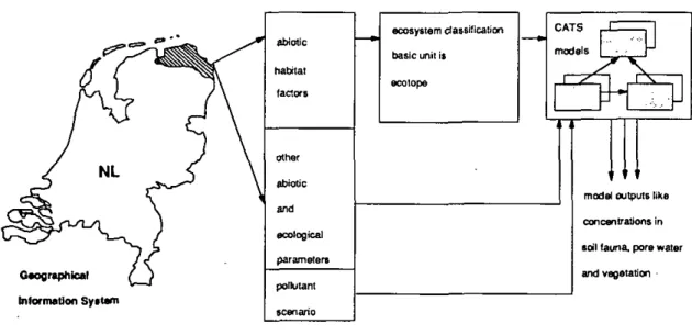
In the frame of the project 'ecological sustainability of the use of chemicals' (PESC), models are being developed that are capable of predicting bioaccumulation of contaminants in aquatic and terrestrial ecosystems (so called CATS models). The goal of this project is the development of an ecotope-based, geographically differentiated model, to predict the efficiency of pollutant-reduction measures.
The term 'ecotope-based* refers to a classification of Dutch ecosystems, according to abiotic and biotic habitat factors for vegetation and soil fauna (Runhaar et al. 1987, Sinnige et al. 1991). Important habitat factors are acidity, productivity, moismre content, salinity and vegetation structure. With these factors, a division of ecosystems in basal units, called ecotopes, can be made. Each type of ecotope is a unique combination of abiotic factors, associated with the species characteristic for that combination.
The term 'model' refers to the entire system as depicted in Fig. 1. The fate and transfer of pollutants in ecosystems will be studied with compartment models, developed for a number of ecotopes. With the aid of the companment model, it is possible to calculate the effect of emission-reduction measures on bioaccumulation in biotic and abiotic compartments of ecosystems. This effect is controlled by the characteristics of that specific ecotope. Thus, the same emission reduction can be effective in one type and ineffective in another.
Geographical Information Sytlani
abiotic
pollutant scenario
ecosystem das silica lion basic unit is ecolope CATS models
n
z
Z ^
& ^ ^ . , •• f " model outputs like concentrations in soil fauna, pore water and vegetationFig. i Diagram of the PESC project, including CATS models. LxKation specific model predictions can be depicted with a CIS system.
When the entire system has been realized, it should be possible to follow the path as illustrated in Fig. 1. First, location-specific information on abiotic habitat factors and other information relevant for modeling, should be collected. The ecotope-type determines which ecosystem model should be used and what additional information is required to be able to run the model. From this stage on, pollutant-reduction measures can be evaluated in terms of change of concentrations in soils, vegetation and fauna or effects on ecosystem functioning. In the later stages of the project, maps of model predictions on concentrations or risk-levels can be drawn using a CIS. At the moment of writing, the system has not been completed yet, a number of the most important modules however, i.e. ecosystem classification and compartment modelling have been reaHzed (Sinnige et al., 1991 and Traas & Aldenberg, 1992).
At the Centrum of Milieukunde of the university of Leiden (CML) a method is developed to assess the risk of persistent chemicals for terrestrial vertebrates due to soil contamination (Eibers & Traas 1992). The method consists of five different parts (Fig. 2). First, the composition of the foodweb of specific vertebrates is analyzed, and aggregated into groups. Second, Bioaccumulauon Factors are collected for these groups, to calculate the concentration in the prey items of the raptor. Third, the diet compostion of a predator, given as the percentages prey items in the diet, determines the average concentration in the food of the predator. It is very easy to vary the diet composition according to regional diet differences. Fourth, the average concentration in the animal is calculated, and compared with an NOEC for internal body concentra-tions with simple accumulation models. Fifth, the calculated concentration is compa-red with an NOEC -for internal concentrations, to assess whether the vertebrates experiences some effect.
The method is strongly based on the assumption that bioaccumulation factors (BAFs) should be considered stochastic variables, since the authors state that BAFs cannot be considerd constant. (In aquatic ecotoxicology studies, one usually speaks of a bioconcentration factor (BCF). Since bioaccumulation does not necessarily leads to biomagnification (cf. Van Straalen 1987), we prefer the use of the term BAF in terrestrial ecosystems.) The distribution of BAFs for specific groups is derived from the open literature, assuming that they are a sample from all possible BAFs for that specific group. Monte Carlo simulations have been performed to calculate the probability distributions for the concentrations in prey items, and finally the concentration in the vertebrate, or organs of the vertebrate. With the resulting internal concentration, the probability that the NOEC is exceeded at a given soil contamination level can be calculated. It is also possible to calculate the maximum permissible concentration, which is that soil concentration that does not lead to more than 5% exceedance of tiie internal NOEC of a specific vertebrate. This MPC has
been calculated for kestrels (Falco tinnunculus). Roe deer (Capreolus capreolus), bam owls (Tyto alba) and weasels (Mustela nivalis) for cadmium, lead and lindane. At present, the method is being validated and a sensitivity analysis will be performed.
The shaded area is not protected, i.e., exceeds tha NOEC
Monte Carlo eimulations to calculate internal concentrations
probab'lity distribution of average food concentration
diet compos tion
determinas average^ncentration
probability distritxition of BAFs at second trophic level
probality distribution of BAFs at first trophic level
•BAF •BAF
Fig. 2 Diagram CML-method
1.3 Proposed research for the raptorial foodweb
The review of related research has shown that simple food chains have been succesfully modelled. More complex foodwebs have also been modelled, but the aim was not specifically directed at raptors.
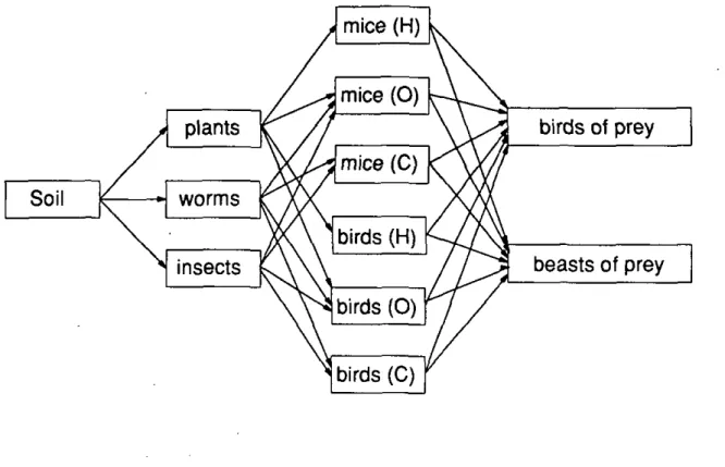
The aim of this project is to develop a general algorithm for effect assessment of effects from secondary poisoning in a terrestrial foodweb: soil via plants and invertebrates to small mammals and birds to birds and beast of prey. A simpHfied
form of such a foodweb can be depicted as follows: mice (H) Soil plants worms insects mice (O) mice (C) birds (H) birds (O) birds of prey beasts of prey birds (0)
Fig. 3: Simplified form of the terrestrial foodweb. Abbreviations: H = herbivorous, O = omnivorous, C = carnivorous.
For every step in the foodweb a bioaccumulation factor (BAF) must be assessed. Toxicity data for birds and mammals for certain selected compounds and the composition of the diet of the different groups or species used in the model have to be collected.
As discussed in several meetings with experts and pointed out by Romijn et al. (1991) and Jonkers and Everts (1991) several factors have been held responsible for influencing secondary poisoning:
1 Laboratory/field conversion 2 Normal versus
extreme conditions 3 Caloric conversion
Differences in metabolic rate between animals in laboratory (toxicity tests) and animals in the field. Differences in metabolic rale under normal field
conditions and more extreme conditions (breeding periode, migration, winter, etc.).
Differences in caloric content of the different types of food (e.g. cereals versus worms).
4 Food assimilation efficiency
5 Pollutant assimilation efficiency
6 Relative sensitivity
Differences in the use of different types of food. It is possible that some animals do use their food better than other species. When this is the case a correction factor must be assessed.
Differences in uptake (bioavailability) of a
com-pound that can appear between test animals (surface application of a compound) and animals in the field (compound in tissues).
Differences in biotransformation or detoxification of certain chemical groups between taxonomical groups of birds or mammals.
It is proposed to investigate whether the influence of these factors on secondary poisoning is substantial or not. If this is true for one or several factors, they could be incorporated in the general algorithm for effect assessment. This matter will be discussed in the next chapter. It may not be possible to incorporate some of the factors listed above in a simple algorithm if more elaborate physiological details need to be included. In that case, a more complex compartmental model needs to be considered. The properties of certain classes of compartmental models are discussed in chapter 3.
8
2 Factors influencing ecological and toxic effects 2.1 Introduction
Since the widespread use of polyhalogenaied hydrocarbons like DDT and PCBs and heavy metals like mercury, it has become known that such chemicals are able to resist degradation both in the abiotic and the biotic envhonmenl. Many cases have been reported where these compounds were held responsible for impaired breeding (Marquenie et al. 1986, Opdam et al. 1987) or death of birds of prey and mammals (Koeman et al. 1972).
It was reasoned that these compounds accumulated progressively with each step in the food chain leading to a predator. This led to the belief that topcamivores are at risk because they are exposed through a food chain, with more risk associated with a longer food chain. Since then, this theory has been severely criticized (Moriarty 1983) and alternative hypotheses put forward and tested (Griesbach 1982, Van Straalen & Van Wensem 1986). Over the years il has become clear that a multitude of factors influence the accumulation and effects of pollutants and many models have been used to clarify the influence of these factors. Because of the change in views about bioaccumulation and effects of toxicants, one can choose from a wide variety of models. How to decide which model has to be used?
In the next paragraphs the existing knowledge on effects of toxicants on terrestrial vertebrates is discussed in order to make a hierarchy of models in the next chapter. Il is also discussed at what level of biological organisation one could study and model effects, what kind of effects exist and how these effects come about and are influenced. With this knowledge in mind it is tried to make a model hierarchy, where each model class adresses increasingly more complex questions. In accordance with the goals of a given project, it is possible to chose a suitable model structure from this model hierarchy.
2.2 Hierarchy of effects
The effects of pollutants on venebraies can be studied on different levels of biologi-cal organisation, from the subcellular to the level of the community. Since this is not necessarily the only possible hierarchy (O' Neill et al. 1986), a hierarchy that seems logical for the effects of pollutants will be discussed.
Most ecotoxicological studies focus on the effects of pollutants on individual orga-nisms, a tradition strongly linked to the methodology of toxicity testing. It is generally agreed that effects eventually affecting survival and or reproduction of individuals will in due course affect the fate of the population of that species
(Mori-arty 1983). On the basis of energy budget studies, Kooijman (1985) argued that observed effects of pollutants on growth, uptake or metabolism eventually influence the rate of reproduction of individuals, and so influence a population's size.
Consequently, individual organisms are regarded as the primary unit for studying effects, since we reason that the effects on the next hierarchical level can for the most part be explained from effects on the lowest level.
However, it is not always clear how effects on individuals should be translated to effects on populations. If accumulation of pollutants like cadmium lead to organ disfunction (Ma et al. 1991) , how does this affect survival or reproduction? The same question could be asked for the numerous studies devoted to measuring enzyme inhibition by organophosphorous compounds (e.g. Hill & Mendenhall 1980). Without answers to these questions, it will indeed be very difficult to link sublethal effects of pollutants on individual vertebrates to population effects.
However, if it is possible to translating effects on individuals to populations, the functioning of the community in which the population resides could be studied. The community is seen as the third hierarchical level. Since the toxic effects occur on a lower hierarchical level, i.e. on the individual organism, the only limitation for predicting effects on the interaction between populations is our understanding of the ecology of the ecosystem being studied. This limitation may be quite severe. An important assumption of this type of hierarchy is, that the behaviour of the highest level can be explained from the behaviour of the isolated units at the lower levels. Because ecosystem components can behave rather different in the laboratory when isolated from the intact natural system, the behaviour of the assembly of units called a community may be different from what can be expected (O'Neill et al. 1986). 2.3 Type of effects.
When effects of poUutants become apparent in field studies, the observed effect could be a result of the direct toxic action of the pollutant, but it could also be an indirect effect of a less easy to observe ecological disturbance somewhere in the ecosystem. Therefore, a distiction is made between toxic effects and ecological effects (sensu de Snoo & Canters 1988). The toxic effects of a compound result from uptake of the pollutant, either from the abiotic environment (water, air, soil, etc.) or from food ingested. The uptake of the chemical leads to presence of the compound in the blood or one or several tissues, where il can exert its toxic potential. These toxic effects do not have to become apparent immediately but could be delayed (cf. section 2.4.5).
In this definition, il doesn't matter how the animal is exposed, whether by drinking water, breathing air or through the food chain, the intoxication is a result of the
10
presence of the toxicant in tissues or blood of the organism.
An ecological effect of poUutants is defined here as a change in the resources of a species which form the niche of a species. As a result of its toxic action somewhere in the community, one or several of the resources are altered, like loss of food, shelter or mating sites. At the level of the community then, the toxic effects on populations are direct effects and cause the secondary ecological effects. We would like to make an exeption for pollutant gases causing global changes, for which the causal chain of effects is less clear. The elevation of the CO2 level in the atmosphere does not have a direct toxic effect on biota, but a more general effect on photosyn-thesis and global temperature. CFKs destroy the ozone layer, this causes a general increase of UV-B radiation, and probably both direct toxic effects and ecological effects will result from this.
So, if ecological effects of a pollutant on a single species have to be predicted, knowledge on community structure, community function and toxic effects of the toxicant on species within the community is necessary. However, the mechanistic explanation of ecological effects is hampered by the scarcity of studies on this subject Studies on contaminated ecosystems (Denneman et al. 1987) have shown that community structure and function can change drastically as a result of the pollution. It is much more difficult to observe low level ecological disturbance due to toxicants, against the background of natural variations and fluctuations (Depledge 1990). In many cases, the system has not observed long enough to know which natural variations and fluctuations are occuring in indisturbed systems. Moreover, the observation frequency or the duration of the experiment does not have to match the temporal scale on which the ecological effects occur.
2.4 Factors influencing toxic effects
Several factors influence the degree of toxic effects. In the following they will be discussed using the causal chain from exposure uptake metabolizalion/exretion -sensitivity - to effects, as a guideline.
2.4.1. Exposure
Exposure to contaminants depends firstiy on the presence of the chemical in different environmental compartments (i.e. water, air, food etc.) and secondly on the behaviour of the organism. Organisms breathing polluted air or living in polluted surface water, cannot avoid exposure.
physico-11
chemical and biological processes governing the fate of the chemical in water, air and soil. Environmental chemisn^ has generated a large body of knowledge to draw from when predicting the fate of the pollutants. However, the fact that a compound is present in environmental compartments does not strictly mean it is available to the organism. The type or organism and its behaviour determine to which environmental compartment(s) it is exposed. Soft-bodied soil organisms such as earthworms may be exposed both through soil pore water (Van Gestel 1991) and by ingestion of food. Insect predators will generally be living in less close contact with the soil, and thus exposure to chemicals will be mainly through food. It is, however, not always clear which compartments are the most important sources of uptake for the chemical, hampering the development of a mechanistic view of the bioavailability of a pollutant.
2.4.2. Uptake
Uptake of chemicals as a result from exposure can be either active or passive. Uptake by passive diffusion across membranes of many chemicals cannot be regulated, like lipophilic compounds that diffuse from the water into algae or fish. Bioconcentration of pollutants in fish can be predicted from the lipophilicity of the compound (Isnard & Lambert 1988, Branson et al. 1975), assuming equilibrium partitioning of the pollutant between water and fat, expressed as K^^. Other pollutants are very similar to essential nutiients, and are assimilated by 'accident*. It is believed that cadmium, because of its similarity to zinc or calcium, is assimilated in this way (cf. Janssen 1991). Pollutants which are in fact nutrients, like phosphorous, copper or zinc are essential and organisms can regulate the uptake and excretion of these nutrients resulting in a more or less constant concentration in the body. The physicochemical properties of the chemical play a role in the rates of uptake. Especially for large molecules, steric parameters such as size, shape and chain length of molecules have been found to be better predictions for bioconcentration in aquatic environments than hydrophobicity (Opperhuizen el al. 1985, Anliker et al. 1981). Depending on the type of pollutant, uptake of a pollutant does not neccesarily have to occur at the same rate. Several factors influencing variations in exposure or uptake will be discussed. 2.4.3. Variations in exposure/uptake leading to variations in dose
1) Spatial variation of exposure.
Il has been shown that within a relatively small area, large differences in exposure to PCBs of Little Owls (Athene noctua) can be found, due to different degrees of environmental contamination (Fuchs et al. 1985). It has also been argued, that
12
vertebrates can act as integrators of spatial variations of exposure (Eijsackers el al. 1985, Denneman i989).
2) Temporal variation of exposure
Seasonal differences in food availability have been observed for many species, both herbivores and predators (Faber & Ma 1986, De Bruijn 1986). Since species that appear in the diet of predators can differ in their accumulation of pollutants, seasonal variations of exposure and uptake can lead to variation in received dose of the predator (Fuchs et al. 1985).
3) Variation in uptake due to metabolic rate differences and different diets.
In this paragraph only results concerning birds are presented, but data for mammals are also available.
The size and weights of the birds in the world are extremely variable (an adult hummingbird weighs around 3 gram and an Ostrich (Struthio camelus) around 122 kg). The percentage of body weight eaten per day (DFI as percent of body weight, based on dry weight) shows a good relation with the body weight (BW) of birds. The log BW = 4.3 - 2.39 * log DFI (after data of Nice presented in Kenaga, 1973. n=19 and R^ = 0.87).
Small birds eat less than large birds, however, in general the smaller the bird the greater the amount of food it eats (by dry weight) on the basis of percent of its body weight (10 gram bird 24% and 1000 gram bird 3.5%). This is in keeping with the increased energy output related to heal loss, necessary because of the increased surface area to body weight ratio of the smaller bird. Small birds also often eat smaller food particles than large birds and so must find and eat more of them.
It is recognized that a difference in the daily rate of food consumption could occur in the diet of a bird, depending on the moisture content and the caloric and nutritive values of its food. Individual variation in the daily rale of food consumption in the field may be due to weather conditions or lack of food. Even under laboratory conditions, Stickel et al. (1965) found that American Woodcocks (Scolopax minor) ate a mean value of 73 (range 11-143) percent of their body weight per day in earthworms (wet weight).
Energy is fundamental to the chemical processes of life. Factors in the balance between energy expenditure and acquisition arc thought to be inextricably linked to the outcome of reproductive bouts during the breeding season and to survival during the winter season.
13
rates, resulting in a high requirement for self-maintenance. Only when the rate of energy acquisition surpasses these self-maintenance requirements this excess energy can be channeled into reproduction. If energy intake is less than expenditure, body tissues are caiabolized, leading to the eventual demise of the animal. Thus, the balance between energy acquisition and expenditure is of pivotal importance in determining the capacities of birds to survive the stresses of their physical environ-ment and to reproduce.
Early work on avian energetics focused to a large degree on the process of thermore-gulation. Birds were captured and placed in laboratory metabolism chambers (MC), and their oxygen consumption or carbon dioxide output was measured at various temperatures. Although these studies led to a number of generalizations regarding the physiology of birds in the laboratory, attempts to extrapolate these findings to the measurement of energy expenditure in wild birds were fraught with uncertainty. While confined to metabolic chambers, birds.neither experience realistic microclima-tes because of the absence of wind and solar radiation nor participate in the same activities as birds in the wild: thus, heat transfer and energy expenditure would markedly different for wild birds compared to birds in the laboratory.
Development in the mid-1950s of the double labelled water (DLW) technique initiated new possibilities for quantification of energy expenditure Field Metabolic Rate = FMR) of free-roaming animals.
Normally 3 different metabolic rates are measured:
- Basal (BMR) Basal or standard metabolism is determined under conditions that usually provide the lowest and most consistent measurement of metabolism, under post-absorbitive conditions, within the thermoneutral zone, whitout activity, and at a particular time du-ring the diurnal cycle.
- Existing (EMR) The existing metabolic rate is the energy needed by an animal when living under laboratory circumstances.
- Field (FMR) The field metabolic rale is the energy needed by free-roaming animals.
All the metabolic rates of birds are very well correlated with the body weight (BW). In table 1 some of the correlations for birds (all species together) are given.
Small birds expend more energy per unit of body mass than large birds. Koteja (1991) was able to compare FMRs and BMRs. FMR tends to increase with increasing body mass slower than BMR, but the difference was not significant. FMR(raising young) tends to increase with increasing body mass faster than the
14 FMR(not raising young).
Table 1 Correlations between body weight and metabolic rate for birds.
Regression
log BMR = 0.55 + 0.668 * log(BW) log BMR^ = 0.558 + 0.673 * log(BW) log BMR^ = 0.583 + 0.624 * k)g(BW) log EMR = 1.286 + 0.529 * log{BW) log FMR = 0.982 + 0.661 • log(BW) log FMR^ = 1.160 + 0.651 * log(BW) log FMR^ = 1.145 + 0.530 * log(BW) Method MC DLW DLW MC DLW DLW DLW n 23 8 127 38 23 8 r^ 0.97 0.96 0.99 0.90 0.95 0.89 References
Lawiewski & Dawson, 1967 Koteja, 1991 Koteja, 1991 Kendeigh et a!., 1977 Williams, 1988 Koteja, 1991 Koteja, 1991
1 = raising young, 2 = not raising young, N = number of species.
The EMR should be lower than the FMR. However, in the case of birds not raising young the FMR is lower than the EMR and thé FMR for birds raising young is higher than the EMR. A possible explanation for this discrepancy is the difference between the methods. There are indications that the estimates of energy metabolism by oxygen comsumption may differ from DLW measurements by up to 50% in birds and mammals (Nagy, 1987).
2.4.4 Factors of concern by extrapolation of laboratory results to field
1) Metabolic rate of animals under laboratory conditions versus animals in field situations.
The large majority of toxicity tests with birds and mammals are carried out under laboratory circumstances. The metabolic rate under laboratory conditions will be lower than the metabolic rate in the field. When using laboratory data for effect assessment in the field a correction factor could be applied.
2) Metabolic rate of animals under normal field conditions versus more demanding circumstances.
15
other activities, aerial-feeding birds may have a higher FMR than birds that use alternative foraging modes, such as ground foraging and flycatching.
Using data from studies that estimated the energy expenditure of adults while feeding nestlings, allometric analysis shows that, in general, aerial-foraging species expend more energy per unit of body mass than species that employ more conservative foraging modes (Williams, 1988).
Although no studies have directiy quantified the FMR of female birds during the period of egg synthesis, indirect calculations suggest that egg laying could be a task of high energy demand for female birds. On average the energy cost for egg synthesis is 0.5 * BMR (Williams, 1988).
Raising young is assumed to increase the chance of parental mortality in much of life-history theory. For a wide array of invertebrates and vertebrates, studies concur that reproduction negatively influences parental longevity. Among bird species, the picture is less clear. One notion is that as nestlings mature, their energy demands increase, requiring parents to bring food to the nest more ft-equently. Along with more feeding nips, parental energy expenditure increases because of increased flight time, resulting in a loss in body mass and ultimately in an increase in the probabiHty of death. The above hypothesis suggests that the FMR of the parents should increase. Positive correlations between FMR and nest visitation have been found for House Martins (Delichon urbica). Starlings (Sturnus vulgaris) and female Savannah Sparrows (Ammodramus sandwichensis). These findings do not mean that in every case a trade-off between brood size and parental mortality will be found. On the contrary, resource levels differ from year to year, and it could be that only during years when resource levels are below some critical value mortality events will increase because of the cost of reproduction (Williams, 1988). Koteja (1991) was able to differentiate between birds raising young and birds not raising young. The energy factor (EF) between FMR(raising young) and FMR(not raising young) for birds is:
log(EF) = log(FMR raising young) - log(FMR not raising young) = 0.015 +0.121 *log(BW)
The FMR of adult Yellow-eyed Juncos (Junco phaeonotus) remained fairly constant throughout the entire breeding cycle, averaging 73.8 kJ/day. Foraging only 75% of the day when they were feeding young, adults did not appear energy limited. In contrast, the FMR of fledgling juncos that are still fed by the parents increased steadily with age, from 59.7 kJ/day during the first week out of the nest to 73.9 kJ/day during the third week. After abandonment by parents, the FMR of independent juveniles increased, peaking at 100 kJ/day in 10- to 12-week-old birds.
16
Apparently, energy balance during this period of early independence is critical to the survival of young birds. To satisfy their energy demands, young juveniles foraged over 90% of each day. Yet in spile of this extended foraging period, almost half of all young juveniles perished, apparently from starvation (unpublished study of Weathers and Sullivan cited in Williams, 1991).
3) Delayed toxicity
Another point of concern are periodes with extreme circumstances, i.e. periodes when the energy intake is less than expenditure, because one could expect delayed toxicity because of use of the fat reserves. Lipophilic compounds can accumulate in fatly tissues of animals. When the animal is experiencing food shortage due to time of year, migration or starvation, these fat reserves are consumed and the stored pollutant ^ is released into the bloodstream. Strong evidence has been found that birds of prey foraging on contaminated Woodpigeon (Columba palumbus) become intoxicinated during winter as a result of fat metabolism (Koeman et al. 1968). In the sixties mortality of seabirds was noticed in the 'Waddenzee'. Telodrin, discharged in the 'Botiek' area, found its way to the mussels in the 'Waddenzee' and to the fatty tissues of the Eider {Somateria mollissima). During the breeding periode this duck does not eat and the fat reserves are resorbed. Eiders were found dead with symptoms typical for lelodrin poisoning (Compaan 1992).
4) Caloric conversion
Most of the (chronic) toxicity tests concerning birds are carried out with repre-sentatives of the group of Galliformes. The fodder given to the tests birds consists of cereals. The mean caloric content of this fodder is 14654 kJ/kg fodder (mean value ^ for cereals in the "Voedingsmiddelentabel"). Most birds of concern (birds at the top
of a food chain) are carnivorous. To estimate the chronic toxicity under field conditi-ons the caloric value of the cereal diet should be converted to 'meat' equivalents. As an example the caloric contents of several other types of food are given in Table 2. The correction factor for cereals to fish would be 14654/4731 = 3.1.
5) Assimilation efficiency a) Food assimilation efficiency
Metabolized energy (ME) in a diet is the total (gross) energy in a unit of food consumed minus the energy lost as faeces and urine resulting from that unit of food. Metabolizable energy efficiency (the ratio ME/total energy, or the fraction of gross
17
Table 2 Caloric contents (kJ/kg) of several types of food.
Category energy content wet weight (kJAg)
source
meat (moderate fat) fish (moderate fat) mussel mussel leatherjacket earthwonn caterpillar fly 10467 4731 3014 3856 3980 3390 5600 5870 Voedingsmiddeleniabel Voedingsmiddelentabel Hölzinger, 1977 Hulscher, 1982 Westerterp, 1982 Westerterp, 1982 , Westerterp, 1982 Westenerp, 1982
energy that is metabolized) is relatively constant among different species of mammals and birds that are either carnivorous, insectivorous or granivorous (Nagy, 1987). In herbivorous mammals, metabolizable energy efficiency for cell wall components increases with increasing body mass, because food ferments for longer periodes in large herbivores (Nagy, 1987). However, small herbivores generally select younger and more tender vegetation that contains relatively low amounts of cell wall material, so actual metabolizable energy efficiency tends to be independent of body mass. By combining average values for metabolizable energy efficiency for birds and mammals eating various diets with typical gross energy contents of those diets, Nagy (1987) calculated the following mean metabolizable energy contents (in units of kJ of metabolizable energy per gram of dry matter): insects, 18.7 for mammals and 18.0 for birds; fish, 18.7 for mammals and 16.2 for birds; vegetation, 10.3 for mammals; and seeds, 18.4 for mammals. He estimated an intermediate value of 14 kJ/g for omnivorous mammals and omnivorous and fhjgivorous birds.
b) Pollutant assimilation efficiency
Pollutant assimilation efficiency relative to food assimilation efficiency determines to a great extent bioaccumulation. In most toxicity tests a mixture of the compound and the fodder (surface appHcation) is tested. Animals in the field will be exposed by compounds which are incorporated in the tissues of their prey. Moreover, toxicity tests are often performed with herbivorous species and not with carnivorous species at the top of a food chain.
18
So, three factors influencing pollutant assimilation efficiency can be determined: 1) the food assimilation efficiency of granivorous birds eating grains in the toxicity
tests, could differ from assimilation efficiency of birds of prey eating birds, mice, etc.
2) the pollutant assimilation efficiency of the test animal could differ from the pollutant assimilation efficiency of animals in the field.
3) the bio-availability of the compound could differ between "surface application" and pollutant incorporated in the tissue.
2.4.5 Physiological factors determining bioconcentration 1) Metabolization / excretion
The concentration in an organism is a dynamic factor and results from uptake and loss processes. Depending on the way of exposure and properties of the toxicant, steady state (uptake rate equals loss rate) can be reached within a short lime like hours or days but also may take years. The loss processes consist of meiabolization and excretion. Hydrophilic toxicants can be easily excreted by the kidneys and cannot diffuse easily across membranes. On the other hand, lipophilic toxicants are less easy to excrete due to their affinity for fatty tissues and membranes. Because of this affinity, it has been shown that the body burden of certain organisms like eel rises with rising fat content (Larsson et al. 1991).
Excretion will. requirc biotransformation into less lipophilic products (Henderson 1986, Walker 1990). All biotransformations and detoxifications require specialized enzyme complexes, like the Mixed Function Oxidase (MFO). The activity of these enzymes can differ widely between different taxa. Many seabirds like cormorants and razorbills have low activities of the Mixed Function Oxidase (MFO) relative to mammals and other birds. A low MFO activity could explain bioaccumulation of polychlorinated hydrocarbons in these organisms (Knight & Walker 1982).
At the population level, the same uptake/loss processes take place, but toxicant mass is now divided over many individuals. New animals are bom and animals die or are predated on. This means that models at the population level should consider these loss processes that influence the average concentration of the toxicant in the populati-on.
2) Body size
Animal sizes may contribute much to the variability among BCFs and make differen-ces between species seem unimportant (Griesbach et al. 1982, Davies et al. 1984).
19
Many physiological processes depend on body size, hke food intake, productivity and respiration. Allometrical relations exist that allow the estimation of a variety of processes for classes of animals related to body size (Peters 1983). This means that bioaccumulation and turnover of pollutants can be expressed as a function of body size (Van Straalen & Van Wensem 1986, Van Straalen 1987).
2.4.6. Sensitivity
Once the pollutant has been absorbed or assimilated, the toxic compound is present in the organism and can exert its toxic potential. This does not necessarily mean, however, that the mere presence of the compound results in a toxic effect on the organism. The compound could be stored in a tissue or an organ where it is not harmful or it could be made chemically inactive. Therefore, organisms that accumula-te more are not necessarily more sensitive or resistant than organisms that accumulaaccumula-te less (Van Straalen 1988). Several processes related to the Hfe cycle of the animal or the state of its environment can influence the sensitivity of the organism or the population:
1) Intra- or interspecies differences.
Large intra- or interspecies differences in sensitivity exist, though laxonomically related species have similar sensitivity to the same chemical (LeBlanc 1984, Van Gestel 1991). Within a population, animals in certain life stages may be more suscep-tible to the compound than in other stages, contributing to the intra-species variation. 2) Food availability
It has been made plausible that in situations of low food availability, populations are more sensitive to effects on reproduction than in situations of ample food (Kooijman 1985). Moreover, on the basis of experiments with poUutants on daphnids, Kooijman & Metz (1984) argue that populations regulated by their food supply, like most predators including birds of prey, are more sensitive to effects on reproduction than populations regulated by these predators.
If the combination of low food availability and toxic effects on reproduction should affect the population size of predators, this phenomenon partly explains the sensitivity of predators to pollutants without the need for an explanation solely on the basis of the length of the food chain.
20 2.5 Factors Influencing ecological effects
The ecological effects resulting from toxic effects somewhere in an ecosystem can be influenced by many factors depending on the structure of the ecosystem:
- Degree of functional redundancy, i.e. the way in which other species can compen-sate for the functions of poisoned species. This abiUty of ecosystems depends on the stability of the ecosystem and whether the foodweb is loosely connected (simple) or highly connected (Pimm el al. 1991).
- Resilience of the ecosystem. Toxic effects of pollutants can go by unnoticed at the level of the ecosystem, because compensating mechanisms operate, Hke recolonization or a high reproductive capacity of the sensitive species leading to a quick recovery. The same toxic load can cause effects in another ecosystem, because of a different foodweb, adverse abiotic conditions or different proces rates. This complicated mix of ecosystem relations determines the resilience to change.
Ecological effects can take place on a short temporal scale, like the loss of cover for animals after herbicide spraying. Other ecological effects, Hke genetic adaptation due to selection pressure may take years. Due to succesion, invasion, natural catastrophes etc, ecosystems are dynamic entities. This causes rearrange-ments of relations and fluctuations in the size, dispersion and composition of populations within the system. Against this background, ecological effects that lake some time to develop, may be hard to detect.
21 3 Modelling the effects of pollutants 3.1 Introduction.
In this chapter the hierarchy of effects mentioned in section 2.2 will be followed, and a consideration is made of what kind of model could be used to predict accumulation and effects at the hierarchical levels discerned. First the modelling of effects at the level of the individual will be discussed, then at the level of the population and finally at the level of different types of food chain or foodweb. Because of the large amount of available models, it is not pretended to review all existing models, nor to tie all existing model classifications together in one scheme.
3.2 Modelling effects on individual organisms
If the individual organism should be protected, effects of pollutants should be modelled. The model structure depends on both the availability of toxicological data and our knowledge of (ecological) factors that influence effects of pollutants. The more attention is payed to the relations of the organism with its environment, the more difficuU it will be to model effects at the level of individual organisms, because interactions between organisms usually are envisioned at the level of interacting populations.
The use of BAFs is a customary black box approach. The only prerequisite is the availability of measurement of concentrations to calculate the BAF. No additional physiological information is needed. When more detail is required because of physiological differences between species in laboratory and field or factors mentioned on page 5, compartment models are needed. Depending on the detail of information and knowledge, a simple one-compartment model or a more elaborate multicompartment model can be used.
3.2.1 Using BAFs to predict concentrations in organisms
Toxicological data like LD50s, LC50s and NOECs can be used to estimate a NOEC for a cenain group of birds or mammals (Romijn et al. 1991a, 1991b). On the basis of protection and risk criteria, a maximum permissible concentration in air, water, soil, or food could be derived (Romijn et al. 1991a). In order to calculate such a maximum permissible concentration il is necessary to consider how and by which routes the animal is exposed. Bioaccumulation factors are used to estimate food chain transfer between different trophic levels. Because it is not necessary to model physiological mechanisms like uptake and elimination, this is essentially a black-box approach (Fig. 4A). With this method the impact of exposure and food intake on
22
effects can be determined. Statistical methods such as regression analysis can be used to establish empirical relations between factors that are believed to influence toxicity and the toxicity data (Romijn et al. 1991b).
! \ LC90, LDSO orNOEC no bioaccumjlalion LCSO, LD50 orNOEC no l>JoacaimjiBi)on •gMton •xeraton A.B.C: Individuals •gMBori moftdily D,E,F: Populations
all loss processes
Fig. 4 Schematic overview of models for bioaccumulation by individuals (A,B,C) or by populations (D,E,F).
A,D: no physiological information is needed.
B,E: general physiological information is needed but no internal structure is present.
C,F: genera] physiological information is needed and internal stmcmre is present.
The concentration in the organism can be predicted by assuming homogeneous distribution of the chemical. If the concentrations in the medium of exposure and in the organism are known, the bioaccumulation factor (BAF), sensu Walker (1990), can be determined.
For a reliable prediction, it is necessary that the BAF is determined when a steady state is reached (Connel 1988). By using BAFs to predict concentrations in otiier simations, no structured processes are available in the model that determines the rate of accumulation. If it is necessary to know the influence of factors on the value of the BAF, empirical relations have to be established between the factors and the BAF (Ma 1982, Van Rooij et al. 1988, Romijn et al. 1991a,b). This may well be the
23
fastest way to describe the influence of many factors on accumulation.
In aquatic ecotoxicity studies, numerous investigations showed high correlations between log K„» and log BCF. Consequently, the hydrophobicity concept (Branson et al. 1975, Isnard et al. 1988) appears to be appropriate for the estimation of bioconcentration in aquatic environments. However, the estimation of the BCF based on log KQ^ is not always reliable because of scatter of BCF values around the regression Hne, and because of dependency on the applied regression method (Davies & Dobbs 1984). Moreover, most BCF regression methods have been calculated for uptake of polyhalogenated organic compounds by fish, which exhibit a structural resistance against metabolization. In general, physiological factors determining bioaccumulation are not adequately delt with when using BCFs to predict bioaccu-mulation (Erikson & McKim 1990). Since all of these objections are also valid for terrestrial habitats, it has been argued that BAFs should not be considered as constants, but rather as stochastic parameters (Eibers & Traas 1992). Moreover, in terrestrial systems many animals are not exposed to the pollutant by passive diffusion from a medium. In those cases. Eibers & Traas argue that the use of constant BAFs is unsuitable for risk assessment.
3.2.2 One-compartment models
In many cases, it is desirable to predict the concentration or body burden of pollutants in organisms, especially when no BAFs are available. Even when effects are not known, it is necessary to know the concentration for calculating accumulation or for calculating food chain transfer. In many risk assessments, it is assumed that the concentration within an organism is in steady state with the enviromenial concentration. Since this is often not xrut the dynamics of the accumulation process have to be determined. In both cases, it is assumed that the pollutant is distributed homogeneously over the entire organism and therefore only a one-compartment model is needed. The only toxicokinetic processes considered are uptake and elimination (Fig. 4B). With this type of model, it is possible to construct anything from very simple to very complex models.
When no BAFs are known, or description of physiological processes is required, the dynamics of accumulation can be described with a one compartment model (Carson et al. 1983). This pharmacokinetic approach has been shown to be of use in bioaccumulation studies (Janssen 1991) and risk assessment and should enhance the understanding of bioconcentration at a mechanistic level. With the aid of this kind of model bioaccumulation can be predicted if exposure and the kinetic parameters for uptake and elimination are known or can be estimated. If the physiology of the animal has not been modelled in detail, only elimination and clearance rates are
24
needed in order to calculate the rale of change in body burden of an animal (dP/dt), in this example exposed through its food:
dP_ dt
^ - K s - c r ^ - K i - P
where k^ is the assimilation efficiency of the pollutant [-], R the ingested ration [gt' '], Cf the concentration of pollutant in the food, k^^ the elimination rate (f') and P the body burden of the animal.
If the influence of the physiology of the organism on the extent of bioaccumulation has not been modelled, uptake and elimination have to be described as functions of the physiology. This will be illustrated with the model of Norstrom et al. (1976) developed for predicting bioaccumulation by fish. They argued that pollutant biokinetics should be coupled to energetics of the organism. Consequentiy they incorporated equations for more complicated metabolic mechanisms within a simple one-compartmental model. Metabolic rate (Q) determines uptake from water and food and is corrected for growth. Elimination is seen as influenced by body weight (W) not influenced by metabolic rate. The simplified differential equation for the rate of change of body burden is
^ = * „ / C ^ • « ( 0 ) + *„„• C„• V(0,0) -k^,-P•ƒ(HO
where in addition to the former formula, food ingestion (R) is a function of metabo-lism (Q). Uptake from water is the second part of the equation with k^u the efficiency of pollutant transfer across the gills [-], C„ the concentration of pollutant in water and V the volume of water flowing past the gill per unit time, as a function of metabo-lism (Q) and oxygen content of the water (O).
Food chain effects are not significant up to log K^^ of 5. For log K ^^ of 5-7, calculated and observed field concentration factors in top predators indicate significant elevations above calculated field BCF values. Above log K^w 7, food chain effects are sensitive to the chemical assimilation efficiency and phytoplankton BCF (Thomann, 1989).
3.2.3 Multicompartment models
Several pollutants have been shown to accumulate in specific tissues or organs. It has been suggested that lipophilic pollutants can enter the bloodstream from the storage tissues when the lipids are needed for energy. To assess the risk of accumulation of
25
these pollutants, and to calculate the concentrations in the appropriate tissues a multicompartiment model is applied. In general, such a model consists of a number of interrelated compartments, conceptually representing organs or tissues (Fig. 4C). If a NOEC for a concentration in a tissue or an organ (MacNicol & Beckett 1985, Ma et al. 1991) is available, it can also be determined whether the calculated concentration should be considered harmful or not. From a model analysis performed with existing data, Moriarty concluded that the fit of multicompartment models to the data hardly ever justifies the use of more than two or three compartments (Moriarty
1983). However, very complex models have been built like that of Kjellstrom and Nordberg (1978). An excellent review on the construction, use and analysis of multicompartment models has been given by Carson et al. (1983).
Varations in üpophilic pollutant accumulation could be explained by the supposed influence of migration, reproduction and starvation on lipid metabolism. Consequent-ly, il is interesting to develop multicompartment models that incorporate these mechanisms. Analogous to the one compartment model, we may now try to express parameters for uptake, distribution and clearance rates as functions of metabolism, weight etc. Such a model has been developed for aquatic organisms by Kooijman and Van Haren (1990). They distinguished four companments:
- an aqueous volume
- a non-aqueous volume of body structure
- a non-aqueous volume of stored energy reserves - a non-aqueous volume set aside for reproduction
The xenobiotic is supposed to be partitioned by diffusion over the water phase, body structure and the lipid fractions. Two partition coefficients are employed, one for partitioning between water and lipids and the other for partitioning between water and body structure. Uptake and elimination are assumed to be proportional to surface area of the animal. The compartment model is linked to a physiological one descri-bing feeding, storage, growth and reproduction. The amount of lipid reserves depends on the feeding condition of the animal and this should be reflected in bioaccumu-lation of lipophilic toxicants.
This interesting model could well be used for developing a terrestrial variant. However, several factors should be taken into account. Instead of diffusion, food intake will be the major pathway of entrance. Since feeding is part of the physiolo-gical submodel, this should not be a major difficulty. Elimination is assumed to be proportional to surface area, which may be true for aquatic animals but as a rule not for terrestrial animals. As the authors state, the physiology of experimental animals is not well described in the literature, impeding rigorous testing of the model.
26 3.3 Modelling effects on populations 3.3.1 Introduction
Most of our knowledge on the toxicity of chemicals is derived from toxicity testing on individual organisms. An assessment of the ecological relevance of these effects implies that the reaction of populations to the toxicant is more important than that of individual organisms. To be able to deduce population effects fi^om effects on individuals at least ecologically relevant criteria like growth, mortality and reproduction should be used. Moreover, we should take into account that populations consist of individuals with different weight, metabolism or sensitivity. One could assume that the sensitivity of a population to a compound is the same throughout the population, but it is also possible that sensitivity differs between individuals in a population. In Fig. 5A a population is depicted with juveniles that are much more sensitive than adults. So, averageing the sensitivity, as deduced from toxicity testing on adult individuals, may not be of great importance to the survival of the population as a whole. Whether a population wiH decline or not, depends largely on factors like
of
toxicity body burden
average
T r
B
average
1 — \ — r
population age classes population weight classes /
age classes
Fig. 5 Population heterogeneity with respect to sensitivity (A) and bioaccumulation (B).
27
its reproductive succes and its fitness relative to other affected populations (Depledge 1990). Prediction of effects on populations on the basis of routine toxicity testing on individuals cannot neglect these factors, as argued by Van Straalen (1987).
The sensitivity of a population as a whole could be assessed with micro- or meso-cosm smdies, furnishing a population LD50, LC50 or - preferably - NOEC (Fig. 4D). These criteria could be used to derive a maximum permissible concenu-ation in air, water, soil or food. Due to size restrictions, these experimental approaches are not applicable for top-predators. So, population toxicity measures from routine toxicity testing are not available for most large terrestrial animals.
If toxicological mechanisms within the population are not modelled, the
use of population toxicity measures can be a phenomenological approach of toxicant effects in a food chain (Van de Meent et al. 1990). This model, type II according to Douben & Aldenberg (1991), will be discussed in the foodweb modelling section. Several ways of modelling effects on populations (unstructured and structured) exist, which will be discussed below.
3.3.2 Unstructured population models
In many models for transport and cycling of toxicants within a system, animal populations are represented as a homogeneous compartment (without internal structure). Fluxes going to the population are uptake of toxicant from water, air or food, fluxes coming from the compartment are egestion, mortality and predaiion (Fig. 4E). Often no explicit population model can be found explaining population behaviour (Griesbach et al. 1982, Wiersma et al. 1984). Consequently, the toxicant present in the companment cannot influence population dynamics since there is no mathematical formalism to do so. It is however possible to use general population models such as the logistic growth equation for the derivation of a population model that can incorporate the effects of toxicants on population dynamics (Hallam et al. 1983, Traas & Aldenberg 1992). In the model of Hallam et al., the equations for the behaviour of toxicant and those for the population are coupled by birth and mortality dose-response functions.
The logistic equation implies that all individuals are identical. As has been mentioned before, this may not be true with respect to susceptibility to the pollutant or body burden. More complicated models have been constructed that take these intra-population differences into account.
3.3.3 Structured population models
Structured population models have been devised to translate the effects on individuals to populations. Since individuals within a population may differ with respect to their
28
sensitivity to the compound, an internal structure is needed to predict population effects. Fig. 4F shows a schematic presentation of a population with internal structure. Within the population different classes according to age or size can be distinguished. Since bioaccumulation can differ between individuals of different life stage or weight, a structured model could also be used to predict the bioaccumulation and pollutant turnover of the population. So there are at least two motives to analyze population structure.
1) Effects on populations
To study the importance of the afore mentioned non-homogeneity of populations, structured population models can be designed. They serve to relate physiological effects of pollutants on individuals to population effects. Thus the model is strucmred according to variables of individual organisms, like weight, length or age. If the population is structured according to age, life stages are often used, like eggs, juveniles, young adults and adults in the case of Daphnid models (Nisbet et al. 1989,
Kooijman et al. 1989). Since the population model is the sum of the processes of individuals within life stages, different characteristics to each life stage like metabolism, reproductive effort or mortality can be ascribed. Toxic effects of pollutants do not have to affect all life stages in the same way. Effects of pollutants on processes of individuals eventually result in a quantitative change of population processes.
These models have been developed for species well studied like Daphnids, or are purely theoretical (Calow & Sibly 1990). At the moment, these models are needed for the construction of ecotoxicological theory (Van Stt-aalen 1988) but are too demanding for a general risk analysis.
2) Bioaccumulation of populations
Structured models can also be used to accurately calculate the turnover of pollutants by a population, relative to its biomass turnover. Van Straalen (1987) developed a weight-structured model for soilfauna that accumulate heavy metals during lifetime. Older (heavier) organisms have a higher body burden than younger animals, that is they accumulate during life time (accumulation sensu law). This may, but does not have to, lead to a steady increase of body concentration (accumulation sensu stricto) during its life time. If individuals primarily die old, animals with a more than average body burden leave the population (Fig. 5B). If individuals primarily die young, biomass leaves the population with a less than average body burden. Unstruc-tured population models cannot distinguish between these different cases. If predators prey selectively on large (old) individuals, they will receive a significantly higher