Environmental (in)equity in the Netherlands - A case study on the distribution of environmental quality in the Rijnmond region

(1)

RIVM Report 550012003/2004

Environmental (in)equity in the Netherlands

A Case Study on the Distribution of

Environmental Quality in the Rijnmond region H Kruize and AA Bouwman

Erratum (see page 2), September 2004

This investigation has been performed by order and for the account of RIVM, within the framework of project S/550012, ‘Population and Health’, and by order and for the account of the Ministry of Public Housing, Physical planning and the Environment (VROM-DGM-LMV) within the framework of the RIVM-project M/830950, ‘Policy-Supporting Instruments’.

(2)

page 2 of 82 RIVM report 550012003

Erratum for RIVM rapport nr. 550012003

Due to improper coding of data the percentages for ‘Accumulated noise level less than 50 decibels’ and for ‘Available public green areas’ in Table 4.1 on page 25 are wrong. The new percentages do not lead to other conclusions in this report. The statement that environmental quality is worse in the Rijnmond region compared to the Netherlands in general holds.

The correct percentages are:

the Netherlands not weighted weighted Accumulated noise level less than 50

decibels (dB(A)) 24.9 36.9

Available public green areas < 50 m2_per

(3)

Abstract

As a part of a broader investigation on environmental inequity in the Netherlands, an exploratory case study on the socio-economic distribution on (perceived) environmental quality was carried out in the Rijnmond (industrial and urbanised) region in the western part of the Netherlands. Disparities in local environmental quality with respect to noise, air

pollution, availability of public green areas, safety risks, and presence of waste disposal sites, were analysed separately and accumulatively across income levels making use of zip codes. Inhabitants’ perception of environmental quality with respect to spatial and income

differences was also ascertained and analysed. Recent, available national and regional

databases and literature were used for the analyses. Disparities in local environmental quality were found to be linked to income level, especially for air pollution and the availability of public green areas. In addition, accumulation of environmental ‘goods’ (high-quality

environmental conditions) were found more often in high-income than in low-income areas. Inhabitants of Rotterdam also mentioned littering and dog mess to be the greatest

environmental problem. All income categories experienced annoyance, but from different, often area-specific sources. Considering these results, policy-makers are advised to take into account the effects of their policy on different income categories.

(4)

(5)

Preface

In 2000, the National Institute for Public Health and the Environment (RIVM) stated in the National Environmental Outlook that quality of the local environment in the Netherlands is often worse in the older urban neighbourhoods, compared to newer neighbourhoods in rural areas (e.g. National Environmental Outlook 5, 2000). These older urban neighbourhoods are often inhabited by lower income people. As a result of these findings the RIVM wanted to explore if low-income people are indeed exposed to a worse environmental quality in their neighbourhoods compared to high-income people in the Netherlands. Therefore, they performed an exploratory research if there were any differences in local environmental quality between zip code areas with a different income level. The results, as presented in the Environmental Balance of 2001, indicated that low-income areas were built more densely, were situated more often in the proximity to a road were the NO2 standard was exceeded, and

were exposed to higher noise levels than high-income areas (RIVM, 2001). To get further insight in this issue of so-called environmental inequity in the Netherlands, the RIVM and the Copernicus Institute for Sustainable Development and Innovation (Utrecht University) started a PhD project on this topic. In this project, performed by Hanneke Kruize (RIVM), the socio-economic differences in local (perceived) environmental quality and causes of these

differences are analysed, with an emphasis on the effects of (environmental) policy. The case study presented in this report is a part of that project, and is still ongoing. Therefore we do not suggest giving a complete insight on the issue of environmental equity in the Netherlands in this report. It rather serves as a discussion document.

Many colleagues at the National Institute of Public Health and the Environment (RIVM) and the Utrecht University have been involved in the case study so far in providing data or knowledge. Among these people are the advisory committee of the doctoral research (Professor N.D. van Egmond (RIVM), Professor dr. P. Glasbergen (Utrecht University), Dr. P.J.J. Driessen (Utrecht University), Dr. M. Kuijpers (RIVM), Dr. A.E.M. de Hollander (RIVM) and Dr. R.van der Wouden (Dutch Spatial Planning Agency)), and Rebecca Stellato (RIVM, statistical expert). We would like to thank all of them for their useful help and hope we may ask for their help in the future again.

This report is an adapted version from the paper presented at the OECD Workshop on the ‘Distribution of Benefits and Costs of Environmental Policies’ organised by the National Policies Division, OECD Environment Directorate (OECD, 4-5 March 2003, Paris). We thank the OECD for the opportunity to take part in this workshop and for their useful comments.

(6)

(7)

Samenvatting

In het kader van een verkennend casusonderzoek naar de sociaal-economische verdeling van lokale (ervaren) milieukwaliteit in de regio Rijnmond zijn verschillen in lokale

milieukwaliteit geanalyseerd voor geluid, luchtverontreiniging, beschikbaarheid van groen, risico’s door industriële activiteiten en vuurwerkopslag, en aanwezigheid van

afvalverwerkingsbedrijven voor postcodegebieden met een verschillend inkomensniveau. Daarnaast is de beleving van de milieukwaliteit van bewoners vastgesteld en geanalyseerd op ruimtelijke verschillen en verschillen tussen inkomensgroepen, en is de relatie tussen de ‘objectieve’ milieukwaliteit (bijv. geluidniveaus, aantal woningen binnen een risicocontour) en ‘subjectieve’ milieukwaliteit (bijv. geluidhinder, onveiligheidsgevoel door aanwezigheid industrie) verkend. Hiervoor werden ruimtelijke gegevens uit bestaande nationale en

regionale bestanden gebruikt. De ruimtelijke verdeling van de lokale milieukwaliteit en inkomen werd geanalyseerd met behulp van een Geografisch Informatie Systeem (GIS). Verschillen in lokale (ervaren) milieukwaliteit tussen sociaal-economische groepen zijn geanalyseerd op basis van statistische analyses. Voor ervaren milieukwaliteit werden tevens in literatuur gerapporteerde resultaten van lokaal en regionaal onderzoek gebruikt.

Op basis van de resultaten van ons onderzoek lijken gebieden met een hoger inkomensniveau een betere milieukwaliteit in hun directe omgeving te hebben dan gebieden met een lager inkomensniveau, met name met betrekking tot luchtverontreiniging en beschikbaarheid van publiek toegankelijk groen. Verder kwamen positieve aspecten (bijv. aanwezigheid van groen, lagere niveaus van geluid en luchtverontreiniging) vaker tegelijk voor in hogere inkomensgebieden dan in lagere inkomensgebieden. Bewoners van alle inkomensklassen ervoeren hinder, maar wel van verschillende, vaak locatiespecifieke bronnen.

Dit casusonderzoek maakt deel uit van een breder promotie onderzoek naar milieu en sociale ongelijkheid (‘environmental inequity’) in Nederland, met aandacht voor de rol van beleid hierin, en een discussie over bestaande perspectieven ten aanzien van ‘environmental justice’.

(10)

(11)

Summary

As a part of an exploratory case study on the socio-economic distribution on local (perceived) environmental quality in the Rijnmond region, a highly urbanised and industrialised region in the western part of the Netherlands, disparities in environmental quality were analysed for noise, air pollution, availability of public green areas, safety risks, and presence of waste disposal sites for zip code areas with a different income level. Furthermore, perceived environmental quality of the inhabitants was assessed and analysed on spatial and income differences, and the relation of perceived environmental quality (e.g. noise annoyance, unsafety feelings due to industrial activities) with environmental quality determined using ‘objective’ indicators (e.g. noise levels, number of dwellings within a risk contour). Spatial data were collected from recent existing national and regional databases. The spatial

distribution of the local environmental quality and income was analysed using a Geographic Information System (GIS). Socio-economic differences in (perceived) local environmental quality were assessed based on statistical analyses. For perceived environmental quality results of local and regional research on this topic, reported in literature, were used as well. The results indicate that disparities were present for zip code areas with a different income level, especially for air pollution and for availability of public green. In addition,

accumulation of environmental ‘goods’ or amenities occurred more often in high-income areas than in low-income areas. Higher income areas thus appeared to have a better environmental quality and showed a higher access to environmental amenities than lower income areas. Furthermore, inhabitants of all income categories experience annoyance, but from different, often area-specific sources.

This case study is a part of a broader investigation on environmental inequity in the

Netherlands, including research on the role of policy in it and a discussion on environmental justice perspectives.

(12)

(13)

1. Introduction

In this chapter the context and the aim of the case study on the socio-economic distribution of (perceived) environmental quality in the Rijnmond region, the Netherlands, is described. Furthermore, the structure of the report is pointed out.

1.1 Context and aim of the case study

In 2000, the National Institute for Public Health and the Environment (RIVM) stated in the National Environmental Outlook that quality of the local environment in the Netherlands is often worse in the older urban neighbourhoods, compared to newer neighbourhoods in rural areas (e.g. National Environmental Outlook 5, 2000). These older urban neighbourhoods are often inhabited by lower income people. As a result of these finding the RIVM wanted to know if low-income people are indeed exposed to a worse environmental quality in their neighbourhoods compared to high-income people. Therefore, they performed an exploratory research on differences in local environmental quality between zip code areas with a different income level. The results, presented in the Environmental Balance of 2001 and below in Table 1.1, indicated that low-income areas were built more densely, were situated more often in the proximity to a road were the NO2 standard is exceeded, and were exposed to higher

noise levels than high-income areas (RIVM, 2001).

Table 1.1 Differences in environmental quality between income categories in the Netherlands

Income category High Above

average Average Low Minimum Mixed Alllevels %

Environmental indicator

More than 35 dwellings per hectare 22 36 49 63 68 46 47 Proximity to green space 17 13 12 13 12 12 13 Infrastructural barrier 9.8 11 11 9.9 9.5 10 10 Proximity to road with NO2 exceedance 16 15 19 27 33 21 20 Noise > 50 dB(A) 80 81 82 84 85 82 82 Noise > 65 dB(A) 3.8 3.7 4.1 4.4 5.3 4.6 4.2 Proximity to ESR/ fireworks1) _0.5 _0.8 _1.1 _1.2 _0.9 _1.0 _1.0

Source: RIVM. RIVM/MC2001

1) ESR establishments and firework storage depots.

To get further insight in this issue of so-called environmental inequity in the Netherlands, the RIVM and the Copernicus Institute for Sustainable Development and Innovation (Utrecht University) started a PhD project. In this project, performed by Hanneke Kruize (RIVM), the socio-economic differences in local (perceived) environmental quality and causes of these differences are analysed, with an emphasis on the role of (environmental) policy. The case

(14)

study presented in this report is a part of that project and is also performed as a part of the OECD (Organisation on Economic Coordination and Development) programme ‘The Social and Environmental Interface: Enhancing the Quality of Life’. The results of this study were used in an OECD workshop on the Distribution of Benefits and Costs of Environmental Policy (March 4-5 2003, Paris) organised as a part of their programme.

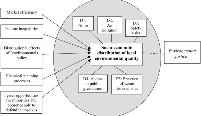
Figure 1.1 is presented to give insight in the part of this case study within the context of the larger research. The grey circle indicates the focus of this case study. It makes clear that the aim of this report is to describe differences between socio-economic groups in (perceived) environmental quality in their neighbourhood, in other words, the socio-economic

distribution of local (perceived) environmental quality. This is both done for separate aspects of environmental quality, such as noise, air pollution and access to public green areas, and for the accumulation of these aspects. Although not explicitly included in this figure, we pay attention to the perception of inhabitants concerning environmental quality in their neighbourhood as well. We will come back to that later in chapter 2.

Distributional effects of (environmental)

policy Market efficiency

Fewer opportunities for minorities and

poorer people to defend themselves Socio-economic distribution of local environmental quality Environmental justice? D4: Access to public green areas D5: Presence of waste disposal sites D1: Noise D2: Air pollution D3: Safety risks Income inequalities Historical planning processes

Figure 1.1. Analytical model for the Rijnmond case study

In this case study we will give special attention to the methodological issues related to analysing the socio-economic distribution of environmental quality. We will give our recommendations on these issues as well. This reports presents the current results of a case study in the Rijnmond region that is still going on. As mentioned before, the case study itself is a part of a larger study on environmental (in)equity in the Netherlands performed at the RIVM and the Utrecht University. Therefore, this report does not suggest giving a complete insight on the issue of environmental equity in the Netherlands and might rather serve as a discussion document for further research.

(15)

1.2 Report structure

The selection and definition of indicators used to describe the socio-economic distribution will be explained in the second chapter. In the third chapter the selected study area is described. The fourth chapter deals with data collection and data availability, and the methods used in this study. The results are presented in different chapters, each chapter describing one topic concerning the socio-economic distribution of environmental quality. Chapter five presents the spatial distribution of the selected indicators. The socio-economic distribution of environmental quality in the Rijnmond region is reported for separate

environmental indicators in chapter six. Chapter seven shows the socio-economic distribution on accumulation of environmental ‘bads’ and ‘goods’. Chapter eight focuses on the

perception of inhabitants on the environmental quality in their neighbourhood and region. Differences in perceived environmental quality between income categories are described, and the association with the so-called ‘objective’ data is investigated. Finally, we discuss the results and methodological issues of this case study and we give an indication what research directions would be interesting to improve the insight in the socio-economic distribution of environmental quality in chapter nine.

(16)

(17)

2. Selection and definition of indicators

2.1 Selection of indicators

The selection of indicators in this report is based on our conceptual ideas, but also on

requirements from the OECD for their workshop (see also p.14). As described in Section 1.1, the aim of the case study was to assess the socio-economic distribution of environmental quality based on empirical data. The OECD requested that the distribution should focus preferably on the household level, and socio-economic categories should in the first place be defined by income. Based on the aim of the case study, we defined two main categories of indicators, namely environmental indicators and socio-economic indicators.

The first category, the environmental indicators, includes the indicators for which a socio-economic distribution was described. Environmental quality might be defined in a strict way, including air quality, soil quality and noise for example, or in a broader way, including

aspects such as availability of public green areas as well. In this case study we chose the latter approach. Most studies included only one environmental aspect, but including more aspects in the same case study gives, in our opinion, a more complete insight in the socio-economic distribution of environmental quality. In addition, it is possible to assess if there are areas with an accumulation of either environmental problems or access to environmental amenities, thus areas where several environmental problems or environmental amenities occur at the same time. Presence of waste disposal sites was added because in American studies on environmental justice the presence of a hazardous waste site is often used as an

environmental indicator. By including this variable we figured we could eventually make comparisons with the results of these studies.

Environmental quality can be described using both ‘objective’ data and ‘subjective’ data. ‘Objective’ data are data that, when generated by different persons using the same methods, are the same. ‘Objective’ data are often used for evaluation or planning processes, for example by policy makers, to get insight in the (predicted) state of for example the local environment. ‘Subjective’ data are important to get insight in the feelings and attitudes of inhabitants about their local environment and in what they consider important in this

environment. These data give insight in the needs of people and the extent to which they are met. This perception is not only related to the ‘objective’ characteristics of the environment, but also to personal and contextual aspects (Van Kamp et al., 2003). Examples of ‘objective’ data are noise levels and square metres of public green areas within a distance of 500 m of each person’s house. Examples of ‘subjective’ data include the satisfaction with the amount of public green areas in the neighbourhood and noise annoyance. We think that including the perception of people adds insight in the role of environmental policy in the occurrence of socio-economic differences in local environmental quality. Furthermore, it might give insight

(18)

in what aspects of the environment should be improved to make the quality of the local environment of people more liveable.

The second category of indicators is the category of socio-economic indicators, defining the socio-economic component for which the distribution is described, in this study being income indicators.

This resulted in the selection of indicators presented in Table 2.1.

Table 2.1 Selection of indicators

Type of indicator Indicator

(‘ Objective’) environmental Air quality

indicators Noise quality

Soil quality

Safety risks from industrial activities, fireworks and transport

Waste disposal sites in direct surroundings

Availability of public green areas (e.g. parks, forest)

Indicators for perceived environmental quality

Perception of environmental quality (air pollution, noise, soil) in the neighbourhood

Perception of availability and quality of public green areas in the neighbourhood

Socio-economic indicator Income

2.2 Making the indicators operational

We made the selected indicators operational, or in other words, we defined them based on several criteria. In the first place, the definition of the indicators should add information to the aim of the case study, namely assessing the socio-economic distribution of environmental quality. In the second place the OECD made a distinction in environmental ‘goods’ (access to environmental amenities) and ‘bads’ (e.g. high levels of air pollution and noise, presence of risky activities).

In addition, we think disparities can be considered in several ways.

• First it could be approached from a very basic ‘protection of general human rights’ level (e.g. defined in the Dutch Constitution). Each Dutch citizen should be treated equally; no distinction should be made based on religion, ethnicity, etc.We translated this into ‘no disparities should exist between income categories in environmental quality’. It might be evaluated by comparing the distributions, means or percentages of each socio-economic category with each other to see if there are differences.

• Second, one could take a minimum local environmental quality at which health and safety are protected as a starting point. Environmental laws and standards may define this

(19)

To analyse disparities, one might compare how often ‘bads’ are present for different socio-economic categories.

• A third approach is that a ‘nice and pleasant’ type of local environment, meaning not only a guarantee for protection of health and safety, but also a type of local environment in which people feel comfortable, a liveable type of local environment. It might be defined as the access to environmental amenities or environmental ‘goods’, things that make people’s local environment a nice and pleasant surrounding. Unless target values are available, a value needs to be chosen to be able to analyse disparities. This value might be set based on expert judgement, or on e.g. surveys on satisfaction or annoyance.

Disparities could then be analysed by comparing how often the present level of an

environmental indicator is below the target value, or the amount of people being satisfied or not annoyed.

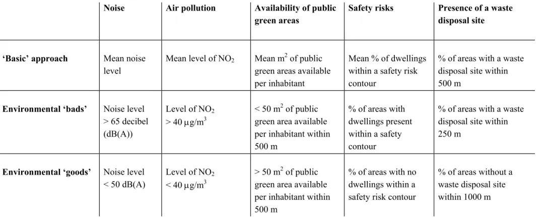
Naturally, the possibilities for defining an indicator in the most optimal way are limited by data availability. The way in which we defined the indicators in this case study is summarised in Table 2.2 and in Appendix 1A and 1B.

(20)

Table 2.2 Definition of indicators for the Rijnmond case study, using three different approaches

Noise Air pollution Availability of public green areas

Safety risks Presence of a waste disposal site

‘Basic’ approach Mean noise level

Mean level of NO2 Mean m2 of public

green areas available per inhabitant

Mean % of dwellings within a safety risk contour

% of areas with a waste disposal site within 500 m

Environmental ‘bads’ Noise level > 65 decibel (dB(A))

Level of NO2

> 40 µg/m3

< 50 m2 of public green area available per inhabitant within 500 m

% of areas with dwellings present within a safety contour

% of areas with a waste disposal site within 250 m

Environmental ‘goods’ Noise level < 50 dB(A)

Level of NO2

< 40 µg/m3

> 50 m2 of public green area available per inhabitant within 500 m

% of areas with no dwellings within a safety risk contour

% of areas without a waste disposal site within 1000 m

(21)

3. The Rijnmond region: general characteristics

The Rijnmond region was selected as the study area for this case study (Figure 3.1). It is a mainport, an industrialised and urbanised area of 800 km2_{in the western part of the}

Netherlands, inhabiting almost 1.2 million people in 18 communities (DCMR, 2002), causing spatial pressure. It also includes one of the largest cities of the Netherlands, Rotterdam. This is a multicultural city, with many minorities from Turkey, Morocco and other North African countries, Suriname, Cape Verdians, and the Antilles. In Rotterdam about thirty percent of the population belongs to these groups of minorities (COS, 2003). Furthermore, the largest industrial harbour of the world is located in this region. Because of the presence of this

harbour there are about 22,000 (industrial) companies of above average size, with activities in the field of chemical products, energy production, and transport, among other activities. The harbour and the industry are mainly located along the ‘Nieuwe Maas’ river, which divides the Region into two parts (Figure 3.1). The harbour is western from the city of Rotterdam. In addition, the region inhabits horticulture, nature and recreation. Furthermore, there is an airport (Rotterdam airport), with 93,170 flights and 826,889 passengers in 2001 (source: Rotterdam Airport), at the northern side of Rotterdam. These activities cause a lot of

transportation on both water and land. There are important highways in the Rijnmond region. As a result, traffic and industry are an important source of pollution in this area. Other

sources of pollution are aircraft, agriculture and horticulture, and the consumer (DCMR, 2002).

The Rijnmond region consists of both heavily urbanised areas as well as rural areas. This potentially results in a higher variety in socio-economic groups and environmental quality than in case one would focus only on the city of Rotterdam, for example. Based on these facts, together with the fact that there appeared to be many useful data, we selected this area. Focussing on a specific area makes it possible to go in more depth and analyse potential causes of the socio-economic differences in local environmental quality in more detail in the future.

(22)

Figure 3.1 Study area: Rijnmond region (‘regio Rijnmond’), with the boroughs (coloured areas) and 4-digit zip code areas (areas within the boroughs) indicated. At the right site the square box indicates the location of the region within the Netherlands.

(23)

4. Data and methods used to describe the distribution of

environmental quality

In the first section of this chapter the process of data collection and data availability is described. In addition, general statistics of the available data are presented on each spatial scale level (6-digit and 4-digit zip code) separately. In the second section methods used to analyse the data are explained generally.

4.1 Data collection and data availability

In order to describe the distribution of environmental quality, quantitative data were collected for the selected indicators (Table 2.1) at the lowest possible spatial scale level, preferably on the household level. If no data were available at that level, the 6-digit zip code level, about the size of a street, was the second option for data collection. This is still a good option, because at this level the differences in local environmental quality for indicators such as noise and air pollutants like NO2 are clearly visible. If no data were available on the neighbourhood

level and 6-digit zip code level, data were collected on the 4-digit zip code level, with the size of several neighbourhoods, and the borough level, with the size of several 4-digit zip code areas. However, at these levels diversity in environmental quality and in income is often wiped out.

National databases, available at the RIVM, were screened for useful data, because this would offer similar data for the Rijnmond region. Furthermore, it would offer the possibility of expanding the analyses to a larger part of the Netherlands, which will be done as a part of the larger environmental equity study mentioned before. In case no data were available from these databases, regional or local data owners were approached. Data were available on different spatial scale levels (see next chapters). Appendix 1A displays the definition of indicators based on the data available at the 6-digit zip code level, the data source and the year of data collection.

For analyses on the 4-digit zip code level 6-digit zip code data on the environmental

indicators were aggregated to the 4-digit level, by averaging the values for all 6-digit zip code areas within a certain 4-digit zip code area. These data were combined with additional data available on the 4-digit zip code level (Appendix 1B). On the 4-digit level the indicator for income could be defined in four different ways, based on the available data. These differently defined income indicators were highly correlated (Appendix 2).

Data on indicators on perceived environmental quality were only available at a higher spatial scale level, namely the level of boroughs (see Figure 3.1). To analyse them in combination with the objective data, we assumed the perceptions available on the level of a borough to be valid for all 4-digit zip code areas within the borough.

(24)

4.2 General description of the available data

Appendix 3 gives a general description of the data. Data were present for 19,495 6-digit zip code areas for most indicators. Table 4.1 shows comparisons of the Rijnmond region with the Netherlands for some of the indicators to get a general idea to what extent the Rijnmond region matches with the Netherlands as a whole. Percentages are presented both not weighted and weighted for the number of inhabitants living in each area to get insight in potential differences caused by weighing. Weighing was applied because in areas with more inhabitants the environmental quality present has an impact on more people.

The average income level is lower in the Rijnmond region compared to the general Dutch population, and the main stage of life per 6-digit zip code area in the Rijnmond region is a little bit younger. In the Rijnmond region the housing density is much higher than in the Netherlands as a whole. In general, environmental quality is worse in the Rijnmond region compared to the Netherlands in general.

Weighted percentages differ a little from the unweighted percentages, and to a larger extent for an accumulated noise level below 50 dB(A) in the Netherlands.

Appendix 4 describes general statistics for many of the indicators for which data were available on a 4-digit zip code level, including the aggregated data on environmental indicators. Data were available on more than a hundred 4-digit zip code areas.

(25)

Table 4.1 Comparisons between the Rijnmond region and the Netherlands on some of the selected indicators (% of 6-digit zip code areas)

Indicator Rijnmond region the Netherlands

Income not weighted not weighted

- high 5.3 8.3 - above average 16.5 23.3 - average 34.0 38.3 - low 20.0 13.4 - minimum 8.3 4.2 - various 7.5 8.7 - unknown 8.5 3.8 Stage of life - starters 1.3 1.3 - young people 5.6 4.2

- couple with young children

21.0 18.6

- couple with older

children 24.2 30.5 - elderly 27.9 29.8 - completed 10.3 10.9 - various 1.1 0.7 - unknown 8.7 4.0 Percentage of areas with a housing density > 35 dwellings/ha

75.1 38.8

not weighted weighted1 not weighted weighted1

Accumulated noise level more than 65 decibels (dB(A))

8.8 7.7 5.4 6.0

Accumulated noise level less than 50 decibels (dB(A))

9.3 10.9 75.1 63.1

Available public green areas < 50 m2 per inhabitant within a distance of 500 metre 87.2 88.8 12.1 13.6 Average percentage of dwellings within a safety contour 5.1 3.8 1.0 1.0

(26)

4.3 Methods of analysis

In general, two methods of analysis were used, namely spatial analyses and statistical

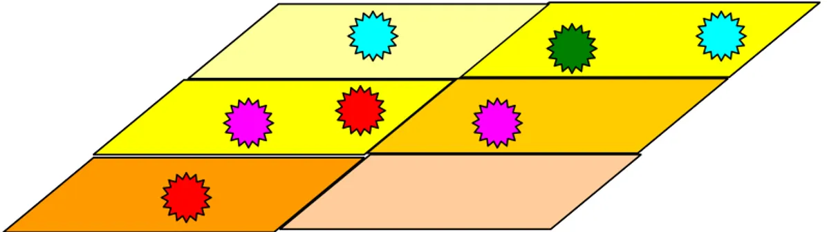
analyses. Spatial analyses were performed in a Geographical Information System (GIS). The available spatial data for each indicator were entered into GIS maps. These maps were used to analyse the spatial distribution of the selected indicators. For some indicators data were already connected with a 6-digit or 4-digit zip code (the units for the statistical analysis). For other indicators, such as noise and air pollution, spatial information needed to be connected to 6-digit zip code for the statistical analysis. This connection was made by overlaying a GIS map with the spatial data of e.g. noise with a map with the 6-digit zip codes. For example, data on noise levels were estimated using a noise exposure model, producing noise levels for 100*100 metre grids. Figure 4.1 shows such an overlay. The ‘stars’ are the 6-digit zip codes, and the squares are the areas with a certain noise level e.g. the noise level in the square in which a certain zip code was situated, was assigned to that zip code. After that, data were read into a statistical software package.

Figure 4.1 Connecting spatial data with 6-digit zip codes

For the statistical analysis we used the statistical software package SAS version 8.2. Most analyses were performed on the 6-digit zip code level, which was considered as the most important scale level for this study. Some additional analyses have been performed on the 4-digit zip code level for analyses for which relevant data were or could only be made available at that level, such as the analyses on perceived environmental quality. For a general description on the socio-economic distribution of environmental quality (cumulative)

frequency tables were produced. The used methods will be explained further in chapters 6, 7, and 8. The results are partly weighted for the number of inhabitants, because in areas with more inhabitants environmental quality has an impact on more people.

(27)

5. The spatial distribution of the selected indicators

Figure 5.1 to Figure 5.6 give examples of GIS maps on the spatial distribution of some of the selected indicators.

Figure 5.1 Spatial distribution of accumulated noise levels (railroad traffic, aircraft, road traffic) in the Rijnmond region

Logically, Figure 5.1 shows that highest noise levels of road traffic, railroad traffic and aircraft were located nearby their sources (main roads, railroads and Rotterdam airport) crossing many different zip code areas. The same was true for NO2, an air pollutant directly

related to road traffic (Figure 5.2, next page). Availability of public green areas seems to be spread over the whole Rijnmond region (Figure 5.3, next page).

(28)

Figure 5.2 Spatial distribution of NO2 concentrations on the pavement in the Rijnmond

region

Figure 5.3 Spatial distribution of availability of public green areas (m2/inhabitant) in the Rijnmond region area by inhabitant 0 m2/inh 1 - 10 m2/inh 10 - 20 m2/inh 20 - 30 m2/inh 30 - 40 m2/inh 40 - 50 m2/inh > 50 m2/inh Availability of public green areas

(29)

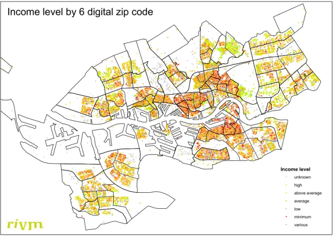
Income level unknown high above average average low minimum various Income level by 6 digital zip code

Figure 5.4 Spatial distribution of income categories in the Rijnmond region

Furthermore, the lower income areas seemed to be concentrated in the centre of the Rijnmond region in Rotterdam, but higher-income areas are present there as well (Figure 5.4).

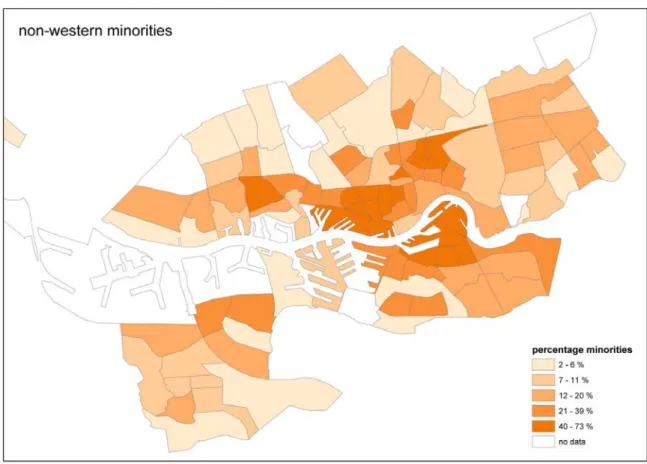
Generally, the same spatial pattern was found for the percentage of minorities (Figure 5.5, next page), with a higher percentage of minorities in lower income areas (Nieuwe Westen, Noord, Centrum, Feijenoord, part of Schiedam). The average house price (Figure 5.6, next page) was highest in the northern and southern areas of the Rijnmond region (Spijkenisse, parts of Vlaardingen and Schiedam, Overschie, Hilligersberg-Schiebroek, Prins Alexander, Capelle aan de IJssel, Kralingen-Krooswijk); the highest housing density was found in the centre of the region, in Rotterdam (Centrum, Nieuwe Westen, Noord, Feijenoord, part of Charlois) (see Figure 3.1 for the location of the mentioned boroughs). It should be noted that data on minorities and on house prices were only available at the 4-digit zip code level. Within these areas there might be differences on these indicators that are not shown because of the less detailed spatial scale level compared to e.g. income (available on 6-digit zip code level).

(30)

Figure 5.5 Spatial distribution of percentage of non-western minorities in the Rijnmond region

(31)

6. The socio-economic distribution of environmental

quality

In this chapter the distribution of environmental quality based on ‘objective’ data is described for different income categories in the Rijnmond region. The first section deals with results on the 6-digit zip code level, presented for each environmental indicator (noise, air pollution, availability of public green areas, dwellings within safety risk contours, presence of waste disposal sites) separately. It starts with a general description of the socio-economic

distribution for the specific environmental indicators, followed by a description in terms of ‘goods’ and ‘bads’, if possible. These results are weighted for number of inhabitants per 6-digit zip code level unless mentioned otherwise. The second section presents some additional results on the 4-digit zip code level.

6.1 A description of the socio-economic distribution of

environmental quality

A. Noise:

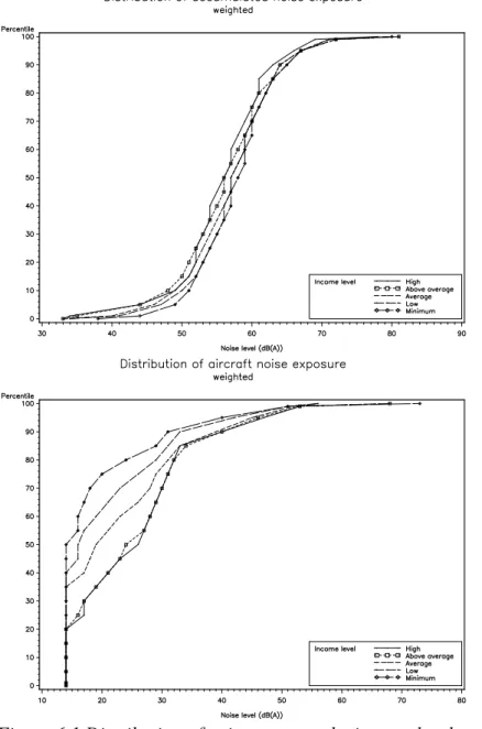
The socio-economic distribution of noise is presented in Figure 6.1 (p.33; note that the scales on the x-axis are different for the different graphs). This figure makes clear that differences between income categories are largest for noise from railroad traffic and noise from aircraft, especially at lower noise levels. Considering the mean noise levels per income category, differences were present for all transportation noise sources, but were largest for noise from railroad traffic and noise from aircraft. The average railroad traffic noise level of lowest income category vs. highest income was 47 vs. 41 dB(A), respectively. For aircraft noise, a reversed trend was found, ranging from 19 dB(A) in the lowest income areas to 25 dB(A) in the highest income areas (Appendix 5).

Railroad traffic noise and accumulated noise (noise from railroad traffic, aircraft and road traffic taken together) showed differences between income categories for noise levels above the Dutch standard of 65 dB(A). For railroad noise the percentage of areas with noise levels above this standard ranged from 0.6% of the highest income category areas climbing to 2.6% of the minimum income category areas, and for accumulated noise from 6.0% climbing to 9.3%.

Concerning noise levels below the Dutch target value for noise (50 dB(A)) we found differences for all noise sources, with the highest income category showing the highest percentage of ‘quiet’ areas, except for aircraft noise, for which the opposite was true. Differences were most pronounced for railroad traffic noise. It appeared that 76.4% of the highest income areas had a noise level below 50 dB(A) compared to 62.5% of the minimum income areas, with the percentage increasing with an increasing income level (Appendix 5).

(32)

Differences were present for accumulated noise as well, varying from 7.5% of the minimum income areas to 11.3% of the high income areas having noise levels below 50 dB(A).

B. Air pollution:

In advance one should be aware that there were many 6-digit zip code areas (54%) for which the concentration was modelled to be zero micrograms/cubic metre (µg/m3_{), mainly because}

NO2 data were modelled only along roads. For 6-digit areas without a road the concentration

was automatically set at zero µg/m3_{. In case all areas including the zero concentration areas}

were used in the analyses, the differences between income categories were more pronounced than for noise (Figure 6.2, p.34, upper graphs; note that the scales of the x-axes are different for the different graphs). Mean levels of NO2 atthe front of dwellings increased with a

decreasing income level, from 12.9 µg/m3_{for high-income areas, to 21.6 µg/m}3 _for

minimum-income areas. For NO2 on the pavement mean levels ranged from 15.7 to 23.9

µg/m3_{, respectively. The percentage of 6-digit zip code areas with NO}

2 levels above the

Dutch standard (40 µg/m3_{) at the front of a dwelling was 5.9% for the highest income areas,}

increasing to 20.6% for minimum income areas (Appendix 6). For NO2 levels on the

pavement this was 17.6% for the highest income areas, increasing to 36.5% for minimum income areas.

When the areas with a zero concentration were left out of the analyses differences were smaller. Average concentrations for NO2 on the pavement varied from 38.8 µg/m3 for the

above average income category to 41.9 µg/m3 _{for the minimum income category}

(Figure 6.2, p.34, lower graphs; Appendix 6). Not the high-income areas, but the above average income areas had the lowest concentrations in this case. Furthermore, 38.4% of the 6-digit zip code areas of the above average income category climbing to 64.0% of the minimum income category had NO2 levels on the pavement above the Dutch standard (40

µg/m3_{). For NO}

2 levels at the front of a dwelling, the concentrations varied from 35.6 µg/m3

in high-income areas to 38.9 µg/m3 _{for the minimum-income category. The percentage of}

areas with levels above the Dutch standard in that case for the minimum income category more than twice the percentage for the high-income category (37.1% vs. 16.3%)

(33)

(34)

(35)

C. Availability of public green areas:

Table 6.1A shows that in higher income areas the average amount of available public green areas (square meters of parks, forests, recreational areas, the number of people with whom one has to share it) is higher than in lower income areas.

Table 6.1 A. Average amount of public green areas (m2) available per inhabitant for various income categories (weighted)

a _{AM: arithmetic mean; sd: standard deviation}

The amount of available public green areas in the highest income areas was 61 m2 per inhabitant compared to 16 m2 per inhabitant in minimum income areas, within a distance of 500 m. 77.8% of the highest income areas did not have 50 m2 within 500 metres distance (‘standard’ for public green areas based on expert judgement). This percentage increased with decreasing income level towards 92.6% of the minimum income areas (Appendix 7).

D. Percentage of dwellings within a safety risk contour:

No clear trend for income was found for this indicator (Table 6.1B). However, Table 6.1B shows that in the highest income areas the percentage was more than three times smaller than in the other areas (1% vs. about 4% respectively).

Table 6.1 B. Average percentage of dwellings within a safety risk contour for various income categories (weighted)

Income category Average percentage of dwellings

within safety contour

High 1.0 Above average 3.8 Average 4.2 Low 3.7 Minimum 3.7 Various 4.3 Unknown 0.4 Income category Distance 200 metres (m) AM (sd)a Distance 500 m AM (sd) Distance 1000 m AM (sd) High Above average 43 (2230) 25 (1500) 61 (3394) 31 (2585) 61 (1615) 41 (3106) Average 17 (939) 23 (1243) 27 (726) Low 12 (587) 17 (1262) 22(1106) Minimum 11 (1077) 16 (1889) 18 (198) Various 17 (396) 26 (480) 31 (622) Unknown 29 (70) 31 (337) 25 (67)

(36)

E. Presence of waste disposal sites:

Table 6.1 C presents percentages of 6-digit zip code areas with waste disposal sites per income category. It shows that the lower the income, the higher the chance to have a waste disposal site in the surroundings of the dwelling, at least at distances of 500 and 1000 metres. No clear trend was found within 250 metres. Only a very small percentage of areas had a waste disposal site within 250 metres.

Table 6.1C. Percentage of zip code areas with a waste disposal site within a certain distance for different income categories (weighted)

Income category Distance 250 m Distance 500 m Distance 1000 m

High 0 0.5 2.5 Above average 0 0.6 4.7 Average 0.3 1.5 6.9 Low 0.3 1.4 7.5 Minimum 0.2 2.2 7.7 Various 0 0.9 6.7 Unknown 0 0 3.2

6.2 Additional results from analyses at the 4-digit zip code level

We performed additional analyses at the 4-digit zip code level with data on socio-economic indicators being available only on that spatial scale level.

Income

To be able to perform analyses on the 4-digit zip code level environmental data on all 6-digit areas within a 4-digit zip code level were averaged. The way in which income data were available at the 4-digit zip code level did not offer a direct possibility to perform descriptive analyses as performed on the 6-digit zip code area. Furthermore, it was not possible to aggregate the income indicator available on the 6-digit zip code level to the 4-digit zip code level, so we could not compare income data from different spatial scale levels directly. Because it was not clear from theories or experience what indicator was best, the four different definitions for income (average income per inhabitant, average income per income recipient, percentage of people of a certain income category, percentage of people with a certain income level; see Appendix 1B) were all used in the analyses. It was not possible to perform descriptive analyses, so instead we performed univariate regression analyses to get some insight in the relation between the environmental indicators and income. These results are not weighted for number of inhabitants per 4-digit zip code area. Weighing, used to adjust for the fact that in areas with more inhabitants the environmental quality present has an impact on more people, does not influence the results in these univariate regression analyses, and was therefore not necessary. Appendix 8 shows the unweighted results of the univariate

(37)

analyses. The income indicators for which the R2 and p-value are bold have the strongest relation with a certain environmental indicator.

For noise the extent to which differences in noise levels were explained by income depended on what definition was used. If the percentage of people within a certain income category was used as the definition of the income indicator, there was a statistically significant (p<0.05) relation between differences in noise levels (all separate sources and accumulated) and income. However, if data on the average income per inhabitant was used, this relation was not statistically significant, except for aircraft noise. Again we found that the higher the income level, the higher the noise exposure, except for aircraft noise, for which agasin the opposite was true.

For air pollution, the negative relation between air pollution levels and income was

statistically significant for all definitions of income, except for income defined as ‘average income per inhabitant’.

For availability of public green areas, it was not clear what income indicator explained most of the differences in the amount of available public green areas, but in most occasions the relation was statistically significant.The higher the income, the higher the amount of public green areas being available per inhabitant.

The percentage of dwellings within a safety risk contour did not show a statistically significant relation with income, independent of the definition of the income indicator. For presence of a waste disposal site within a certain distance did not show statistically significant results either. The association was strongest with the percentage of people of a certain income category at all distances.

Overall, the definition of income with categories instead of continuous data appeared to explain more of the differences in environmental quality between areas, especially when income was defined as the percentage of people of a certain income category (<30, 30-50, 50-80, >50-80,000 guilders/year).

Non-western minorities

Other analyses performed at the 4-digit zip code level concerned the influence of the presence of non-western minorities. This indicator has been used in many American studies on

environmental justice, instead of or together with income. In those studies it is often questioned if it is either income or ethnicity that makes the difference in environmental quality. In the Rijnmond region this is difficult to find out, because income and the

percentage of non-western minorities are fairly strong correlated with each other (correlation coefficient of about 0.7; see Appendix 2), which might result in co-linearity. Appendix 9 shows results of the regression analyses. Significant associations for the association between the percentage of non-western minorities and environmental quality were found for noise from railroad traffic, aircraft noise, air pollution, and availability of public green areas within 500 and 1000 metres, but not for the other environmental indicators. The higher the

percentage of non-western minorities, the worse the environmental quality concerning these indicators.The associations were strongest for aircraft noise and air pollution, in which 25%

(38)

of the variance was explained by the percentage of non-western minorities in a zip code area. The percentage of non-western minorities also influenced the association between income and environmental quality.

6.3 Summary of the results

In general, inhabitants of higher income areas appeared to have more access to environmental ‘goods’ than inhabitants of lower income areas. Furthermore, environmental ‘bads’ were more often present in lower-income areas than in higher-income areas. On the 6-digit zip code level, these differences showed especially for air pollution (the higher the income, the lower the levels of NO2), availability of public green areas (the higher the income, the higher

the amount of availability of public green areas), and for presence of a waste disposal site in the surroundings (the higher the income, the lower the chance of having a waste disposal site in the surroundings). For noise, differences were larger for noise levels below 50 dB(A) compared with noise levels above 65 dB(A), and most pronounced for noise from railroad traffic and accumulated noise. A decrease in income level corresponded with a decreasing percentage of areas with a noise level below 50 dB(A). An exception was found for aircraft noise, for which the opposite was true. For percentage of dwellings within a safety contour, only the highest income category showed to have a lower percentage of dwellings within the safety contour compared to the other income categories.

On the 4-digit zip code level, the association between income and the aforementioned environmental indicators was generally confirmed, with again the strongest relation between air pollution (NO2 levels) and income (negative association), and no clear relation between

percentage of dwellings within a safety risk contour and income. The definition used for income influenced the results found on this scale level, and the percentage of people of a certain income category (< 30, 30-50, 50-80, > 80,000 guilders/year) explained more of the differences in environmental quality between areas in most cases than the income indicators defined in another way. In addition, the percentage of non-western minorities, being highly correlated with income level, was related to local environmental quality as well, especially for aircraft noise and NO2, but also for availability of public green areas. The percentage of

non-western minorities seemed to influence the association between income and environmental quality as well. This might indicate that the presence of non-western minorities is an influential socio-economic indicator, next to income.

(39)

7. Accumulation of ‘bads’ and ‘goods’ and its

socio-economic distribution

In the previous chapters we considered the socio-economic distribution for various environmental quality separately. However, people are often exposed to more than one impact (either ‘good’ or ‘bad’) at the same time in their local surroundings (‘hot spots’). Therefore, we analysed the accumulation of quality in each 6-digit zip code area for both the accumulation of ‘bads’ and the accumulation of ‘goods’. Based on that information policy makers could e.g. determine in what areas measures are needed most urgently.

There are several ways to investigate the accumulation of ‘goods’ and ‘bads’ and to define ‘goods’ or ‘bads’, dependent on the perspective used in and aim of a study. One could for example look at the extent to which the levels for a certain indicator divide from the average level in the community or the average national level, counting the number of problems occurring in a neighbourhood, or one can take the perception of inhabitants, the ranking in importance of indicators, as a starting point. In this case study three levels of accumulation were defined for both environmental ‘bads’ and for environmental ‘goods’, connecting to the perspective presented in Table 2.2. They also might give some insight in the spectrum of ‘minimum quality’ to a ‘nice and pleasant’ local environment, as mentioned in chapter 2. The first level of accumulation was defined based on existing Dutch and European standards for noise and air pollution and might be considered as an indication of a minimum quality environment. The second level included presence of dwellings within a safety contour as well, because this is related (next to noise and air pollution) to health and safety of people, which are often considered as basic issues for which inhabitants should be protected. This is the middle category in the spectrum. The third level is again one step further, including also availability of public green areas, using a standard mentioned by Dutch experts not being implemented in law, and presence of waste disposal sites within a certain distance. These last issues may be considered as ‘extra’ issues, making the local environment nicer and more pleasant for inhabitants, but are not as basic as the issues included in the first two levels. These levels of accumulation are presented in Table 7.1, and explained further below. ‘bads’:

level 1: An accumulated noise level (road traffic, aircraft and railroad traffic) of more than 65 dB(A) and an NO2 level on the pavement of more than 40 µg/m3;

level 2: An accumulated noise level of more than 65 dB(A), an NO2 level on the

pavement of more than 40 µg/m3_{, and dwellings within a safety contour;}

level 3: An accumulated noise level of more than 65 dB(A), an NO2 level on the

pavement of more than 40 µg/m3_{, dwellings within a safety contour, less than}

50 m2 available public green areas within a distance of 500 metres, and presence of a waste disposal site within 250 metres.

(40)

‘goods’:

level 1: An accumulated noise level of less than 50 dB(A) and an NO2 level on the

pavement of less than 40 µg/m3_;

level 2: An accumulated noise level of less than 50 dB(A), an NO2 level on the

pavement of less than 40 µg/m3_{, and no dwellings within a safety contour;}

level 3: An accumulated noise level of less than 50 dB(A), an NO2 level on the

pavement of less than 40 µg/m3_{, no dwellings within a safety contour, more}

than 50 m2 available public green areas within a distance of 500 m, and no waste disposal site present within 1000 m.

Table 7.1 Accumulation of environmental indicators: definition of levels

‘Bads’ ‘Goods’

Level 1 Level 2 Level 3 Level 1 Level 2 Level 3

Accumulated noise + > 65 dB(A) + + + < 50 dB(A) + + NO2 + > 40 µg/m3 + + + < 40 µg/m3 + + Safety risks - + dwellings within a contour + - + no dwellings within a contour + Availability of public green areas - - + < 50 m2_within 500 m - - + > 50 m2 within 500 m Presence of waste disposal sites - - + waste disposal site within 250 m - - + no waste disposal site within 1000 m + included; - not included

We analysed the socio-economic distribution of accumulations of ‘goods’ and ‘bads’, resulting in the distribution presented in Table 7.2. This table shows that the percentage of areas with accumulation of the ‘bads’ is not so large (about 3% for level 1, and 0% for level 2 and level 3). Considering the distribution of ‘bads’ among income categories, there was no clear trend, except that a higher percentage of minimum-income areas had an accumulation of noise and air pollution problems compared to the other areas. The differences in

accumulation of ‘goods’ (Table 7.2), however, appeared to be larger. These results indicate that the higher the income level, the higher the percentage with accumulation of

environmental ‘goods’ in the local surroundings. A subdivision between average to high-income areas and low and minimum-income areas seems to be present.

(41)

Table 7.2 Percentage of zip code areas with accumulation of ‘bads’ or ‘goods’ for different income categories (weighted)

Accumulation of environmental ‘bads’:

Accumulation of environmental ‘goods’:

Income category Accumulation of ‘goods’ Level 1 Accumulation of ‘goods’ Level 2 Accumulation of ‘goods’ Level 3 High 11.2 11.3 3.3 Above average 13.0 12.9 2.5 Average 11.2 11.1 1.0 Low 7.7 7.5 0.2 Minimum 5.9 6.2 0.2 Various 9.9 9.3 1.7 Unknown 5.4 9.3 0 Overall 10.2 10.1 1.2

Furthermore, we looked at the spatial distribution of accumulation of ‘bads’ and ‘goods’. Generally, accumulation of these ‘bads’ was present in the centre of the Rijnmond region, in the city of Rotterdam (Figure 7.1). Accumulation of ‘goods’ showed to be concentrated at the northern and southern borders of the Rijnmond Region (Figure 7.2-7.4, next pages). Amidst areas with accumulation of ‘bads’, there were also some 4-digit zip code areas in the central part, in which accumulation of environmental ‘goods’ was present.

Income category Accumulation of ‘bads’ Level 1 High 3.0 Above average 2.8 Average 2.9 Low 3.6 Minimum 5.3 Various 3.9 Unknown 1.9 Overall 3.3

(42)

Figure 7.1 Spatial distribution of accumulation of environmental ‘bads’, level 1

(43)

Figure 7.3 Spatial distribution of accumulation of environmental ‘goods’, level 2

(44)

(45)

8. Perceived environmental quality in the Rijnmond

region

So far, we only used the so-called ‘objective’ indicators to describe the socio-economic distribution of environmental quality. However, as mentioned in chapter 2, perception of the inhabitants concerning environmental quality in their neighbourhood is relevant as well to get a full insight in the socio-economic distribution of local environmental quality. Perception of people can be considered as the result of the expectations concerning their local environment (‘needs’) and the real situation. For example, if people expect to live in a neighbourhood with a lot of public green areas, and these areas are not available in their neighbourhood, this may result in dissatisfaction about the availability of public green areas in their neighbourhood. This depends not only on the present environmental quality, but also on personal and contextual aspects (Van Kamp et al., 2003).

In this chapter we focus on four aspects. First, we pay attention to the perception of inhabitants of the Rijnmond region in general, and in comparison with the Netherlands. Second, we focus on spatial differences in perception within the Rijnmond region. Third, we describe socio-economic differences in the way inhabitants perceive environmental quality in their neighbourhood. Fourth, we explore the association between ‘objective’ and perceived environmental quality in the Rijnmond region. This will give an idea of differences in perception of the quality of the local environment and environmental quality based on ‘objective’ measures.

8.1 Data sources and methods of analysis

In order to describe the socio-economic characteristics of perceived environmental quality we used two types of data. In the first place we used data from regional or local research

presented in literature. Note that data were available from different surveys performed in different years. In the second place we used the ‘objective’ data on environmental quality and income already described in previous chapters, combined with the interview data from the local statistical agency of the city of Rotterdam, collected between 1997 and 1999 in

Rotterdam. Data on perception of inhabitants were available on the level of boroughs, while data on environmental indicators were available on the 6-digit level. We merged the data on the 4-digit zip code level by using the interview data of the borough for all 4-digit zip code areas within the borough, and used the aggregated environmental data. In some boroughs less than 50 people were interviewed, resulting in unreliable results. Therefore, the results of these analyses should be interpreted carefully. We performed simple correlation analyses

(46)

8.2 Perceived environmental quality in the Rijnmond region- a

general description

In 1998 the Province of South-Holland performed a survey on the perception of inhabitants on environmental quality in their direct surroundings in several neighbourhoods near a harbour or industry, but also among a representative sample of inhabitants in the Rijnmond region. This survey showed that 12% of the Rijnmond population was dissatisfied with the environmental situation in their neighbourhood. In the areas near a harbour or industry this percentage was around 16%. Annoyance due to traffic appeared to be the main unpleasant aspect of living in that neighbourhood, mentioned by 14% of the respondents. At the same time the quietness of the neighbourhood was mentioned to be the most pleasant aspect of living in that neighbourhood by 28% of the inhabitants. Environmental issues in the neighbourhood thus seemed to play an important role for residents in the Rijnmond region initially. However, when asking to what problems in society the government should pay attention, environmental management was only fourth in rank, after health care, security of citizens, and employment opportunities. Before 1990 inhabitants ranked it relatively higher. Furthermore, more people were dissatisfied with space in the streets, public transport and the situation in the streets than with the environmental situation (Table 8.1) (Kamphuis, 1998).

Table 8.1 Percentage of inhabitants dissatisfied with an aspect of their local environment in the Rijnmond region, 1998.

Dissatisfied with: Rijnmond -North1 Rijnmond -South1 Reference Areas Dwelling 11 8 4

Situation in the streets 20 23 17

Space in the streets 22 22 17

People in the neighbourhood 8 10 4

Environmental situation 17 16 3

Facilities in the neighbourhood 11 17 6

Parks etc. in the surroundings 8 9 8

Public transport 21 17 40

Living situation in general 3 5 1

1 _{neighbourhoods near a harbour or industry}

Source: Province of South-Holland, 1998

In addition, satisfaction with the local environment was mainly determined by the extent of satisfaction with the dwelling, followed at distance by the situation in the streets, satisfaction with neighbours and with facilities in the neighbourhood in Rotterdam. The environmental situation and satisfaction with parks showed a much weaker, but significant association with the general satisfaction with the local environmental (Bik, 1999). Nevertheless it was the second issue mentioned to be a problem in Rotterdam by 29% of the participants, after social security (70%) (Luijkx and Rijpma, 2001). In 1990, 39% of the inhabitants of Rotterdam