Energy reduction for autonomous driving through distance-based control

(1)

(2)

distance-based control

Energy reduction for autonomous driving through

Academic year 2019-2020

Master of Science in Computer Science Engineering

Master's dissertation submitted in order to obtain the academic degree of

Supervisor: Prof. dr. ir. Lieven Eeckhout

Student number: 01505243

Wout Klingele

(3)

Preface

As a child, I was always fascinated with futuristic means of transportation portrayed in movies. I was often wondering whether these would become reality, and if I ever would be able to use one of them. Now, almost a decade later, this dream is coming closer within reach than I would ever have expected due to the rapid technological advancements, in particular in the area of autonomous driving.

Once the thesis subjects were published online, I immediately felt drawn towards this subject. Not only was my childhood dream comer closer to reality, but I could also become a part of it.

I am incredibly grateful for the opportunity to investigate this field of the engineering spectrum. The project combined many skills learned during my education, but it also built on top of my existing knowledge. It was a perfect project to end my career at the University of Ghent. On the same note, I am thankful for being able to use the GPU used in this dissertation. Thirdly but of no less importance, I want to thank my supervisor, Prof. dr. ir. Lieven Eeckhout, for his continuous support and guidance throughout the course of this dissertation. His valuable feedback given during our weekly scheduled meetings kept me on track and resulted in a suc-cessful outcome of this dissertation. Furthermore, I would like to express my gratitude towards Lu Wang for helping me with all server-related issues. Apart from all the technical support I received, I also finally want to thank my family and friends for always being there for me and for continuously encouraging me throughout my university career.

(4)

Permission of Use

The author gives permission to make this master dissertation available for consultation and to copy parts of this master dissertation for personal use. In all cases of other use, the copyright terms have to be respected, in particular with regard to the obligation to state explicitly the source when quoting results from this master dissertation.

Wout Klingele, June 2020

(5)

Energy reduction for

autonomous driving through

distance-based control

Wout Klingele

Master’s dissertation submitted in order to obtain the academic degree of Master of Science in Computer Science Engineering

Supervisor: Prof. dr. ir. Lieven Eeckhout Academic year 2019-2020

Faculty of Engineering and Architecture Ghent University

Abstract

The high rise in the interest and the development of autonomous vehicles comes with some very complicated challenges. For instance, autonomous vehicles con-tinuously need to create a perception of the environment by performing various complex algorithms using many different sensors, resulting in a continuous high power consumption. The additional power consumption can significantly reduce the total driving range of a vehicle. Hence, the objective of this thesis is to reduce the energy consumption during autonomous driving by proposing the distance-based control method. The proposed method reduces the amount of sensor data to be analysed by proportionally scaling the frame rate with the vehicle speed. As a result, fewer frames are analysed when travelling slow whereas more frames are analysed when travelling fast. It relies on the philosophy that a slower reac-tion time is justified when travelling slow. A state-of-the-art autonomous driving simulator is used to measure the performance of the new method. The experimen-tal results of this thesis show that the proposed distance-based control method significantly reduces the power consumption during autonomous driving while maintaining a relatively high performance.

Keywords

(6)

Energy reduction for autonomous driving

through distance-based control

Wout Klingele

Supervisor: Prof. dr. ir. Lieven Eeckhout

Abstract - The high rise in the interest and the development of autonomous vehicles comes with some very complicated challenges. For instance, autonomous vehicles continuously need to create a perception of the environment by performing various complex algorithms using many different sensors, resulting in a continuous high power consumption. The additional power consumption can significantly reduce the total driving range of a vehicle. Hence, the objective of this thesis is to reduce the energy consumption during autonomous driving by proposing the distance-based control method. The proposed method reduces the amount of sensor data to be analysed by proportionally scaling the frame rate with the vehicle speed. As a result, fewer frames are analysed when travelling slow, whereas more frames are analysed when travelling fast. It relies on the philosophy that a slower reaction time is justified when travelling slow. A state-of-the-art autonomous driving simulator is used to measure the performance of the new method. The experimental results of this thesis show that the proposed distance-based control method significantly reduces the power consumption during autonomous driving while maintaining a relatively high performance.

Keywords - Autonomous vehicles, perception, CARLA simulator, energy reduction

1 Introduction

Road safety is the main reason why autonomous vehicles (AVs) or self-driving cars are gaining so much traction right now. AVs can minimise the number of road acci-dents due to their better and faster perception, antici-pation and reaction capabilities when compared to ordi-nary manually controlled vehicles. According to the 2019 Urban Mobility Report, an average commuter spends 54 hours in traffic jams each year [1]. AVs can optimise traffic routing to significantly reduce traffic congestion. Apart from the safety and traffic congestion benefits, there exist numerous other reasons why self-driving cars are on the rise such as more time for productivity or relaxing dur-ing your commute, new and better mobility options for elderly and less fuel consumption.

In order for an AV to travel safely through traffic, many different fairly complex tasks need to be executed in parallel. For example, autonomous driving systems (ADSs) should be fully aware of their environment at all times and should be able to react as fast as possible. A lot of different and power-intensive techniques are needed to create a perception of the environment. For example, digital image processing is incorporated in many differ-ent autonomous driving tasks, significantly increasing the total power consumption in ADSs. The total power con-sumption of such an ADS can easily go up to about 1 kW,

considerably reducing the driving range with about 7.59% in a 2018 Audi A4 Ultra. With the current rise in electric vehicles, this problem becomes even worse due to their already smaller driving ranges. For instance, the driving range of a Tesla Model S is reduced by approximately 11.7% considering an additional power consumption of 1 kW.

This dissertation is organised as follows. Section 2 describes the two most important autonomous driving requirements for this dissertation. In Section 3, a new method, the distance-based control method, is proposed to reduce the power consumption during autonomous driving. Section 4 explains the experimental setup for evaluating the performance and the power of the distance-based control method, followed by an analysis of the re-sults in Section 5. Finally, Section 6 concludes this dis-sertation.

2 Autonomous Driving

AVs should be able to safely operate in highly non-deterministic environments. Even though safety is the top priority, AVs can still fail at some point in time. These rare occasions give rise to many different types of chal-lenges ranging from social to legal chalchal-lenges. For ex-ample, according to a study performed by Deloitte, con-sumers are fifty-fifty on whether AVs will be safe [2].

(7)

2.1 Performance Requirements

To ensure safe operation, the ADS should meet strict per-formance requirements. However, determining the safety or the performance of an ADS is not an easy task and is quite vague. An ADS performs better than another ADS when it navigates safer and smoother through traffic. A good indication of the safety of an ADS is the reaction time. If the reaction time of an ADS is fast, then the chances are rather high that the vehicle will be able to operate safely through the road network. The reaction time of the ADS relies on two elements: (1) the frame rate of the ADS and (2) the processing latency of the ADS.

• Frame rate: The frame rate is a measure indicat-ing how fast the sensor data is beindicat-ing evaluated in the ADS. The required frame rate in ADSs is still undefined. Lin et al. [3] require a frame rate of at least 10 frames per second (fps) to continuously adapt to the changing traffic.

• Processing latency: The processing latency mea-sures how fast the processing unit of the ADS can analyse the incoming sensor data. It is the time elapsed since receiving the sensor data and until a control is sent to the actuator of the vehicle. Ac-cording to a study carried out by McGehee et al. [4], the initial steering reaction of a driver occurs on average after 1.64 s. As a result, Lin et al. [3] require a processing latency of maximum 100 ms as the fastest human-capable action requires only 150 ms [5].

2.2 Energy Requirements

An ADS consumes a huge amount of additional energy. This additional energy can significantly reduce the driv-ing range of an AV.

Every additional 1 kW consumed power decreases the fuel economy with about 1 km/L on average in a gas-powered car [6]. For example, in a 2018 Audi A4 Ultra, the fuel economy equals approximately 13.18 km/L [7]. Hence, every additional 1 kW power consumption reduces the driving range with about 7.59%. For example, a com-puting platform operating at full utilisation consisting of one Central Processing Unit (CPU) and three Graphical Processing Units (GPUs), can reduce the driving range with almost 7.59%.

However, most AVs are most likely going to be elec-tric vehicles. Due to the already much smaller driv-ing ranges of electric vehicles, it is even more important to maintain an as low as possible total power consump-tion during autonomous driving. For example, The Tesla Model S has a battery capacity of 100 kWh and a fuel

consumption of 19 kWh/100km, resulting in a maximum driving range of only 526 km [8]. The national average traffic speeds in Europe vary from 34 km/h to 58 km/h [9]. Travelling at an average traffic speed of 45 km/h results in a power consumption of 45km

h × 19 kW h

100km = 8.55 kW.

Finally, every additional 1 kW consumed power thus re-duces the driving range with approximately 11.7%.

Unfortunately, the additional consumed power brings a lot of additional heat with it. Joudi et al. [10] showed that 77% of additional energy is generated to dissipate the heat using a conventional automotive air condition-ing system.

3 Distance-Based Control

In order to reduce the total consumed power during au-tonomous driving, a new method is proposed. The new method, the distance-based control method, reduces the power consumption by simply reducing the number of frames to be analysed by the ADS. Rather than analysing a fixed frame rate expressed in fps, a variable frame rate proportional to the vehicle’s speed is used. The frame rate of the distance-based method is expressed in frames per meter (fpm), the number of frames analysed by the ADS per meter as opposed to the ordinary frame rate expressed in fps. The new method thus analyses fewer frames when travelling slow than when travelling fast. It relies on the principle that a slower reaction is justified when a vehicle is travelling slower. The total stopping distance is in-creased by only a very small percentage when the vehicle is travelling slower, whereas for very high vehicle speeds, the total stopping distance is decreased.

4 Experimental Setup

In order to compare the performance and the power con-sumption between the distance-based control method and the conventional time-based control method, two different types of experiments were carried out: (1) performance experiments and (2) power experiments. Both the per-formance experiments and the power experiments were executed on Nvidia’s GeForce GTX 1080 GPU.

4.1 Performance Experiments

Section 2.1 described two metrics for evaluating the safety of an ADS. The frame rate used in this dissertation is either a distance-based frame rate or the conventional time-based frame rate. However, the processing latency requirement remains the same for the distance-based con-trol method as for the conventional time-based concon-trol method. Lin et al. [3] investigated the processing latency

(8)

of some of the most important autonomous driving algo-rithms.

Therefore, to compare the performance between the distance-based control method and the conventional time-based control method, other performance metrics are needed. Hence, multiple more practical and experimental performance metrics are introduced in this dissertation to evaluate the performance of an ADS such as the average distance travelled until the ego-vehicle crashes, the aver-age time the ego-vehicle spends outside of its restricted lane and the average amount of damage caused by the AV.

All the performance experiments were executed on the CAR Learning to Act (CARLA) simulator [11, 12], a widely used open-source simulator for autonomous driv-ing research. The simulator made it possible to evaluate the performance of an ADS using the practical perfor-mance metrics.

The distance-based control method is implemented as follows. For a frame rate of X fpm, the simulation runs at 60 fps and each first frame detecting a travelled dis-tance of more than 1

Xm since the previous control update

is used to control the vehicle, all the other frames are discarded. Note, when using an fpm-based method, no control updates will be sent to the actuator if the vehicle stands still (for example, when waiting for a red light). In order for the system to keep working at very low driv-ing speeds, a minimum number of one control update per second is introduced.

4.2 Power Experiments

According to Lin et al. [3], the three bottleneck algorithms in autonomous driving are object detection, object track-ing and localisation. As a result, the total power con-sumption of the ADS is simplified to be the sum of the power consumption of the three bottleneck algorithms. However, Lin et al. [3] showed that each of the three bottleneck algorithms consume approximately the same amount energy. Hence, only the power consumed by the state-of-the-art You Only Look Once v3 (YOLOv3) ob-ject detection algorithm is calculated.

The power experiments use the captured images re-trieved from the CARLA simulator during the perfor-mance experiments. The captured images are then fed to a slightly adapted version of the YOLOv3 algorithm. The adapted version analyses the input images at a fixed fpm as opposed to a fixed fps. Simultaneously, the power of the complete system is monitored while the objects are being detected. The complete power draw is estimated using the Nvidia System Management Interface (nvidia-smi) command line utility and is accurate to within ±5 W according to the manual page from Nvidia.

5 Results

Finally in this section, the actual results of the exper-iments are presented. The main goal of this section is to find out whether the distance-based control method is able to reduce the power consumption while maintaining a certain performance.

Section 5.1 shows the performance of the distance-based control method. In Section 5.2, the performance of the distance-based control method is compared to the per-formance of the conventional time-based control method, followed by a comparison of the power consumption in Section 5.3. Finally, Section 5.4 gives an indication of the total reduced driving range.

5.1 Performance Experiments

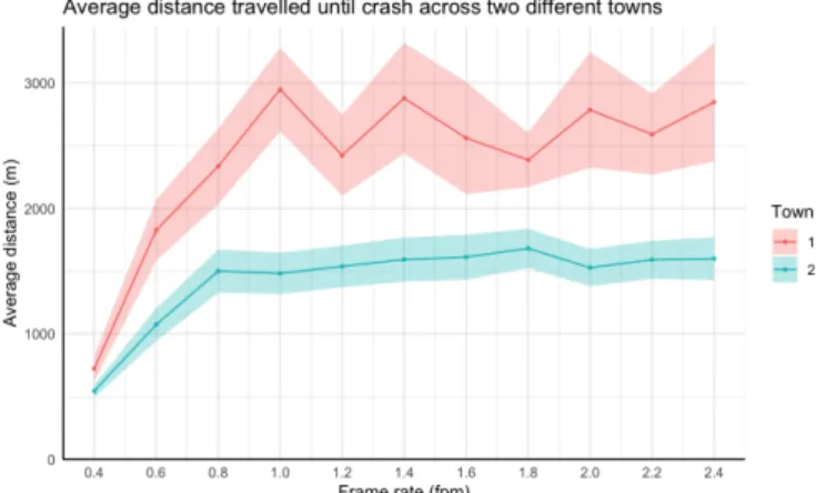
In this section, the performance of the distance-based con-trol method is analysed in function of various different distance-based frame rates. In Figure 1, the most impor-tant practical performance metric is shown, the average distance travelled without crashing metric. The average travelled distance is fairly low for very low frame rates but quickly increases. A frame rate lower than 1 fpm is def-initely not sufficient for controlling an AV. However, the metric starts to stabilise for frame rate values of 1.4 fpm and higher. Hence, a higher frame rate does not really increase the performance of the ADS while significantly increasing the energy consumption. Note that all the ex-periments are performed in an urban environment with a maximum speed limit of 90 km/h. In more rural en-vironments, the optimal fpm frame rate will be a little higher. For this reason, slightly higher frame rates are used throughout the power experiments in order to not exploit the urban environment characteristics.

Figure 1: The average distance travelled by the ego-vehicle without crashing in function of the frame rate expressed in fpm. The two different colors represent two different towns in the CARLA simulator

(9)

In addition, both the average collision intensity and the average successful simulations performance metrics start to converge for the same frame rate values of 1.4 fpm and higher. However, the average normalised time spent outside the restricted lane metric already starts to con-verge for a frame rate of 1.2 fpm or higher.

5.2 Distance-Based versus Time-Based Performance

This section compares the distance-based method with the conventional time-based method. In Figure 2, the av-erage distance travelled without crashing metric is plotted for two towns to compare the performance between the 1.4, 1.8 and 2.2 fpm frame rates and some of the most widely used fps frame rates.

For both towns, the performance of the distance-based method is much better than the performance of the time-based method at 10 fps. However, the distance-time-based per-formance in Town 1 is lower than the time-based 30 fps performance, whereas the distance-based performance in Town 2 is equal to or better than the performance of the higher time-based frame rates. Hence, to ensure an equivalent performance to the 30 fps frame rate, a slightly higher distance-based frame rate needs to be chosen.

Figure 2: A comparison between the distance-based method and the time-based method for the average trav-elled distance without crashing. The two different colors represent two different towns in the CARLA simulator

When using the average collision intensity as a per-formance metric, the distance-based method outperforms the time-based method in Town 2. However in Town 1, only the 2.2 fpm frame rate comes close to the perfor-mance of the 30 fps frame rate, whereas the 1.4 and 1.8 fpm frame rates perform better than the 10 fps frame rate but worse than the 30 fps frame rate.

The average normalised time spent outside the re-stricted lane is the only metric where the performance

of the distance-based and the time-based frame rates are equivalent for both towns.

Finally, the distance-based frame rates again slightly outperform the time-based frame rates in terms of aver-age successful simulations in Town 2. However in Town 1, each of the distance-based frame rates outperforms the 10 fps frame rate but performs significantly worse than the time-based frame rates of 30 fps and higher.

5.3 Power Experiments

After comparing the performance of the distance-based control method and the conventional time-based control method, it is time to look at the actual difference in power consumption. Note that only one out of the three most power consuming autonomous driving algorithms is anal-ysed below as they each consume approximately the same amount of power.

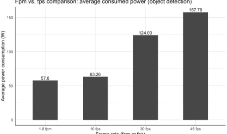
In Figure 3, the average consumed power during the execution of the object detection algorithm is plotted in order to compare the proposed 1.8 fpm frame rate with some time-based frame rates. The second town of the CARLA simulator is used. Note, slightly lower power reductions should be achieved in the first town of the CARLA simulator. It can be observed that the distance-based frame rate at 1.8 fpm consumes less power than the time-based frame rate at 10 fps. Even though, it was con-cluded that the performance of this distance-based frame rate is much higher than that of the time-based 10 fps frame rate. A power reduction of around 8.6% is visi-ble. When compared to either the 30 or 45 fps frame rate, a much higher power reduction is achieved. When comparing the distance-based 1.8 fpm frame rate to the time-based 30 fps frame rate with slightly higher perfor-mance, a power reduction of 53.4% is achieved.

Figure 3: A comparison between the distance-based con-trol method and the time-based concon-trol method for the average power consumption of the object detection algo-rithm.

(10)

5.4 Driving Range Reduction

An ADS with 12 cameras results in a total power con-sumption of approximately 124 W × 3 × 12 = 4.46 kW when using the ordinary method at a frame rate of 30 fps. When using the distance-based control method at a frame rate of 1.8 fpm, a total power of approximately 57.8 W _{× 3 × 12 = 2.08 kW is consumed.}

As a result, for a conventional gas-powered car, the driving range is reduced by 7.59% × 4.46 = 33.85% us-ing a frame rate of 30 fps whereas the drivus-ing range is reduced by 7.59% × 2.08 = 15.79% using a frame rate of 1.8 fpm. Using the distance-based control method in the 2018 Audi A4 Ultra, a total driving range of 137.8 km has been reclaimed when compared to using the time-based control method.

However, most of the AVs are going to be electric ve-hicles. Due to their very limited battery capacities, the impact of an ADS on the driving range is even bigger. A power consumption of 4.46 kW reduces the driving range in the Tesla Model S with approximately 4.46 × 11.7% = 52.18%. Using the distance-based control method, the driving range is reduced by only 2.08 × 11.7% = 24.34%. By incorporating a distance-based ADS in a Tesla Model S, a total driving range of 146.46 km has been reclaimed when compared to using the time-based control method.

6 Conclusion

This work resulted in a total power reduction of ap-proximately 53.4% on a GPU using the distance-based method at 1.8 fpm when compared to using the time-based method at 30 fps. As a result, the driving range reduction is also reduced by 53.4%. However, note that the performance of the ADS is slightly decreased.

This dissertation still leaves a lot of leeway for im-provement and extension. Additional experiments should be performed in more rural environments, on a physical AV and on other processing units.

References

[1] D. Schrank, B. Eisele, and T. Lomax, “2019 Urban Mobility Report,” 2019, p. 41.

[2] J. Vitale Jr., C. Giffi, R. Robinson, S. Schmith, M. Sase, T. Schiller, M. Hecker, R. Singh, and J. H. Bae, “2019 Deloitte Global Automo-tive Consumer Study,” 2019, p. 27. [Online]. Available: https://www2.deloitte.com/content/

dam/Deloitte/us/Documents/manufacturing/ us-global-automotive-consumer-study-2019.pdf [3] S. C. Lin, Y. Zhang, C. H. Hsu, M. Skach, M. E.

Haque, L. Tang, and J. Mars, “The architectural im-plications of autonomous driving: Constraints and acceleration,” in Proceedings of the Twenty-Third International Conference on Architectural Support for Programming Languages and Operating Systems, vol. 53, no. 2, 2018, pp. 751–766.

[4] D. V. McGehee, E. N. Mazzae, and G. H. Baldwin, “Driver reaction time in crash avoidance research: Validation of a driving simulator study on a test track,” Human Factors and Ergonomics Society An-nual Meeting Proceedings, vol. 44, no. 20, pp. 320– 323, 2000.

[5] S. Thorpe, D. Fize, and C. Marlot, “Speed of pro-cessing in the human visual system,” Nature, vol. 381, no. 6582, pp. 520–522, 1996.

[6] R. Farrington and J. Rugh, “Impact of Vehicle Air-Conditioning on Fuel Economy, Tailpipe Emissions, and Electric Vehicle Range,” 2000. [Online]. Avail-able: http://www.nrel.gov/docs/fy00osti/28960.pdf [7] U.S. Department of Energy, “2018 Audi A4 Ultra,” n.d. [Online]. Available: https://www.fueleconomy. gov/feg/Find.do?action=sbs&id=37302

[8] Tesla, “European Union Energy Label,” 2019. [On-line]. Available: https://www.tesla.com/en_EU/ support/european-union-energy-label

[9] M. André and U. Hammarström, “Driving speeds in Europe for pollutant emissions estimation,” Trans-portation Research Part D: Transport and Environ-ment, vol. 5, no. 5, pp. 321–335, 2000.

[10] K. A. Joudi, A. S. K. Mohammed, and M. K. Aljan-abi, “Experimental and computer performance study of an automotive air conditioning system with al-ternative refrigerants,” Energy Conversion and Man-agement, vol. 44, no. 18, pp. 2959–2976, 2003. [11] A. Dosovitskiy, G. Ros, F. Codevilla, L. Antonio,

and K. Vladlen, “CARLA : An Open Urban Driving Simulator,” CoRL, pp. 1–16, 2017.

[12] ——, “Open-source simulator for autonomous driving research.” 2017. [Online]. Available: https://github.com/carla-simulator/carla

(11)

Contents x 2.3.1 Sensing . . . 13 2.3.2 Perception . . . 13 2.3.3 Planning . . . 13 2.3.4 Control . . . 14 2.4 Sensors . . . 14 2.5 Perception . . . 17 2.5.1 Object Detection . . . 17 2.5.2 Object Tracking . . . 18 2.5.3 Localisation . . . 19 2.6 Planning . . . 20 2.6.1 Route planning . . . 20 2.6.2 Prediction . . . 20

2.6.3 Behaviour and Trajectory planning . . . 20

2.7 Control . . . 21

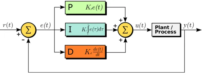
2.7.1 Proportional Integral Derivative (PID) Control . . . 21

2.7.2 Model Predictive Control (MPC) . . . 22

2.8 Computing Hardware . . . 23

2.8.1 CPU . . . 23

2.8.2 Graphical Processing Unit (GPU) . . . 23

2.8.3 FPGA . . . 24

2.8.4 ASIC . . . 24

2.8.5 Specialised Autonomous Driving Computing Platform . . . 25

2.9 Upcoming Autonomous Driving Architectures . . . 27

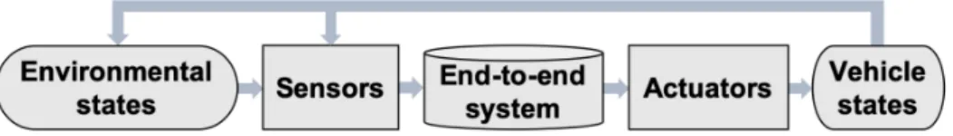
2.9.1 End-to-End Systems . . . 27

2.9.2 Vision-Based Autonomous Driving Architecture . . . 28

3 Distance-Based Control 30 3.1 Stopping Distance Analysis . . . 30

3.2 Problem Statement . . . 31

3.3 Solution: Distance-Based Control . . . 34

4 Experimental Setup 37 4.1 Hardware Setup . . . 37

4.2 Performance Experiments . . . 38

4.2.1 CARLA Simulator . . . 38

(13)

Contents xi 4.2.3 Experiments Configuration . . . 40 4.2.4 Implementation . . . 43 4.2.5 Limitations . . . 44 4.2.6 Runtime Analysis . . . 45 4.3 Power Experiments . . . 46 4.3.1 Localisation Challenges . . . 46

4.3.2 Object Tracking Challenges . . . 47

4.3.3 Object Detection Challenges and Setup . . . 47

4.3.4 Implementation . . . 47

5 Results 49 5.1 Performance Experiments . . . 49

5.1.1 Average Distance Travelled Without Crashing . . . 49

5.1.2 Average Collision Intensity . . . 52

5.1.3 Average Normalised Time Spent Outside the Restricted Lane . . . 54

5.1.4 Average Successful Simulations . . . 55

5.2 Distance-Based versus Time-Based Performance . . . 56

5.2.1 Average Distance Travelled Without Crashing . . . 56

5.2.2 Average Collision Intensity . . . 57

5.2.3 Average Normalised Time Spent Outside the Restricted Lane . . . 58

5.2.4 Average Successful Simulations . . . 59

5.2.5 Conclusion . . . 60

5.3 Power Comparison . . . 60

5.4 Theoretical Driving Range Reduction . . . 62

6 Conclusion and Future Work 64 6.1 Conclusion . . . 64

(14)

List of Figures

1.1 The six levels of driving automation according to the SAE. . . 3

2.1 Power consumption and driving range reduction of the Audi A4 Ultra incorpo-rating different computing platforms. . . 11

2.2 Modular autonomous driving pipeline . . . 12

2.3 Typical sensors in an HAV with their corresponding functionality. . . 15

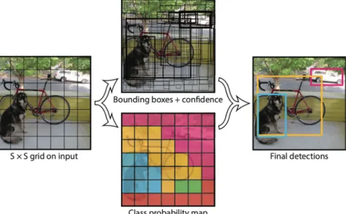
2.4 YOLOv3 3-step methodology . . . 18

2.5 PID control loop diagram . . . 21

2.6 End-to-end system flow diagram . . . 27

3.1 The stopping distance can be observed in function of the vehicle speed. . . 31

3.2 99.99th-percentile latency of the three most power consuming autonomous driving tasks . . . 32

3.3 Power consumption of the three most power consuming autonomous driving tasks 33 4.1 Four different images captured from the two built-in urban towns of the CARLA simulator. . . 39

4.2 The two CARLA simulator components. . . 40

4.3 Random pedestrian behaviour across three different simulations. . . 41

4.4 Comparison of two simulations with a different number of spawned pedestrians. . 42

4.5 Two images showing the impact of adding (many) highly non-deterministic vehi-cles to the simulator. . . 43

5.1 Average distance travelled until crash across two different towns. . . 50

5.2 Average simulation time travelled until crash across two different towns. . . 52

5.3 Average collision intensity across two different towns. . . 53

5.4 Average normalised simulation time the ego-vehicle spent outside of the bounds of the restricted lane across two different towns. . . 54

5.5 A histogram indicating the percentage of successful simulations in function of the frame rate. . . 55

(15)

List of Figures xiii

5.6 A comparison between the distance-based control method and the time-based control method for the average travelled distance without crashing. . . 57 5.7 A comparison between the distance-based control method and the time-based

control method of the average collision intensity. . . 58 5.8 A comparison between the distance-based control method and the time-based

control method of the normalised time spent outside of the restricted lane. . . 59 5.9 A comparison between the distance-based control method and the time-based

control method of the number of successful simulations. . . 59 5.10 A comparison between the distance-based control method and the time-based

control method for the average analysed frames per second. . . 61 5.11 A comparison between the distance-based control method and the time-based

(16)

List of Tables

2.1 Comparison of fuel consumption and fuel economy between an ordinary gas-powered car and an electric vehicle. . . 10 3.1 A comparison of four processing units (CPU, GPU, FPGA and ASIC) for

au-tonomous driving. For each category the preferred processing units are shown in bold. . . 33 4.1 Specifications of Nvidia’s GeForce GTX 1080 GPU. . . 37

(17)

Abbreviations

ACC adaptive cruise control

ADAS advanced driver-assistance systems ADS autonomous driving system

ASIC Application-Specific Integrated Circuit

AV autonomous vehicle

BDS BeiDou Navigation Satellite System BSD blind spot detection

CARLA CAR Learning to Act

CNN Convolutional Neural Network CPU Central Processing Unit

CUDA Compute Unified Device Architecture

DARPA Defense Advanced Research Projects Agency

DET object detection

DNE Deep neuroevolution

DNN Deep Neural Network

FPGA Field-Programmable Gate Array

fpm frames per meter

fps frames per second

FSD Full Self-Driving

GLONASS GLObal NAvigation Satellite System GNSS Global Navigation Satellite System GPS Global Positioning System

GPU Graphical Processing Unit

HAV highly autonomous vehicle

HD High Definition

(18)

Abbreviations xvi

HDL Hardware Description Language HLS High-Level Synthesis

IMU Inertial Measurement Unit

km/L kilometres per litre

L/100 km litres per 100 kilometres LIDAR Light Detection and Ranging LKA lane keeping assist

LOC localisation

MPC Model Predictive Control

NPU Neural Processing Unit

nvidia-smi Nvidia System Management Interface

OpenCL Open Computing Language

PID Proportional Integral Derivative

RADAR Radio Detection and Ranging

SAE Society of Automotive Engineers

SLAM Simultaneous Localisation and Mapping

SoC System-on-Chip

SONAR Sound Navigation and Ranging

TRA object tracking

(19)

1

Introduction

According to a recent study, the average American spends nine hours per week driving a car, which equals spending around 18 days per year in a motor vehicle [1]. Unfortunately, driving a motor vehicle is among the most dangerous activities performed on a daily basis. For young people, aged between 5 and 29, road accidents are the main cause of death [2]. Worldwide 1.35 million lives are taken in road accidents every year.

Another interesting fact is that approximately 94 percent of the tragic road crashes are caused by human errors [3]. Such human errors include speeding, distracted driving, driving under the influence of alcohol or drugs, illegal manoeuvring, etc.

1.1 Context

Road safety is the main reason why autonomous vehicles (AVs) or self-driving cars are gaining so much traction right now. AVs can minimise the number of road accidents due to their better and faster perception, anticipation and reaction capabilities when compared to ordinary man-ually controlled vehicles. According to the 2019 Urban Mobility Report, an average commuter spends 54 hours in traffic jams each year [4]. AVs can optimise traffic routing to significantly reduce traffic congestion. Apart from the safety and traffic congestion benefits, there exist nu-merous other reasons why self-driving cars are on the rise such as more time for productivity or relaxing during your commute, new and better mobility options for elderly and less fuel consumption.

It becomes pretty clear why autonomous driving is getting so much traction. In order to further encourage and accelerate the research and the development in autonomous driving, the Defense Advanced Research Projects Agency (DARPA) organised three autonomous driving competi-tions. Each of these competitions awarded the winner a generous prize. The first challenge was organised in 2004 and took place in the Mojave Desert. The AVs needed to follow a 240 km long traject, however none of the vehicles were able to finish and no one received the one million US Dollar prize. The AV Sandstorm of Red Team from Carnegie Mellon University travelled the furthest of all the vehicles with a disappointing travelled distance of 11.78 km. Even though the

(20)

Context 2

first DARPA Grand Challenge seemed to be a failure, it raised a lot of interest and spurred tech-nological advancements in the area of autonomous driving. These techtech-nological advancements were already noticeable during the second Grand Challenge. While during the first challenge no AV was able to complete the course, five AVs finished the 212 km long course of the second challenge and only one out of the 24 vehicles travelled less distance than the winner of the previous Grand Challenge. The Stanford Racing team from Stanford University won the 2005 Grand Challenge prize of two million US Dollars with their AV Stanley, it came in after driving for six hours and 54 minutes. In 2007, DARPA organised their third and latest autonomous driving competition. However, this time the vehicles needed to complete a shorter 96 km course but in an urban environment complying to the traffic rules. This time it was the AV Boss from Carnegie Mellon University’s team Tartan Racing who came in first and claimed the two million US Dollar prize. Stanford University’s team Stanford Racing claimed the second place with their AV Junior. The DARPA challenges gave rise to many other competitions being organised which were all inspired by the DARPA challenges.

A lot of companies saw an opportunity and invested big money in the research and the devel-opment of self-driving cars. However, it should be noticed that every car on the market today still requires the driver’s engagement. This is due to the fact that getting a fully autonomous vehicle on the market is not just about manufacturing the vehicle itself. Some of the major challenges concerning autonomous driving are: meeting strict safety requirements, complying with the law, persuading the public to use AVs, and finally the engineering of the vehicle it-self. Due to these challenges, the movement towards complete automation happens gradually and occurs in multiple phases. The gradual process creates more trust and a safer feeling from the users towards autonomous driving systems (ADSs). The Society of Automotive Engineers (SAE) distinguishes six levels of driving automation ranging from absolutely no automation to complete automation [5]. The six different automation levels can be observed in Figure 1.1. In summary, cars belonging to level 0 are to be controlled completely manually. Automation levels 1 and 2 are characterised by their advanced driver-assistance systems (ADAS) such as adaptive cruise control (ACC), lane keeping assist (LKA) and blind spot detection (BSD). These func-tionalities introduce partial automation into vehicles but the driver is still the main source of control. From level 3 onwards high driving automation is considered, the driver is no longer the primary source of control.

Various definitions exist concerning ADSs. In this thesis, a vehicle from level 1 onwards and a vehicle from level 3 onwards can be considered as an AV and a highly autonomous vehicle (HAV), respectively. The main focus in this thesis will be put on HAVs as these depict the self-driving cars with high to full automation.

(21)

Problem Statement 3

Figure 1.1: The six levels of driving automation according to the SAE. Source [5]

More and more car manufacturers are incorporating ADASs into their vehicles helping the driver to perform specific actions or manoeuvres in order to reduce road accidents and the driver’s burden. Most AVs on the road today belong to automation level 1, for example cars with ACC. Vehicles with multiple ADASs can be considered automation level 2, for instance a vehicle with both ACC and LKA. One of the main examples of such a level 2 ADS is the Tesla Autopilot used in for example the Tesla model S. The Audi AI in the Audi A8 was the first ever ADS to reach automation level 3 under certain conditions. Unfortunately, the Audi A8 was not able to make use of the level 3 automation because of legal issues. There are no commercially available AVs with an automation level of 4 or 5. However, Waymo is already test-driving their HAV of level 4. Other promising self-driving car companies are Intel’s Mobileye, GM’s Cruise, Argo AI, Lyft and Uber.

1.2 Problem Statement

In order for an HAV to travel safely through traffic, many different fairly complex tasks need to be executed in parallel. For example, ADSs should be fully aware of their environment at all times and should be able to react as fast as possible. A lot of different and power-intensive techniques are needed to create a perception of the environment. For example, digital image processing is incorporated in many different autonomous driving tasks, significantly increasing the total power consumption in ADSs. The total power consumption of such an ADS can easily go up to about 1 kW, considerably reducing the driving range with about 7.59% in a 2018 Audi A4 Ultra. With the current rise in electric vehicles, this problem becomes even worse due to their already smaller driving ranges. For instance, the driving range of a Tesla Model S is

(22)

Objective 4

reduced by approximately 11.7% considering an additional power consumption of 1 kW.

1.3 Objective

The main objective of this dissertation is to reduce the energy consumption during autonomous driving by simply reducing the number of frames to be analysed by the ADS. In this dissertation, a new method is proposed, the distance-based control method. The proposed method analyses a frame at each distance interval as opposed to analysing a frame at each fixed time interval. Hence, the number of analysed frames scales linearly with the speed of the vehicle. A slower travelling vehicle uses less frames to control the HAV when compared to a faster travelling vehicle. The method is based on the philosophy that a slightly slower reaction time is justified when travelling at lower speeds and a faster reaction time is needed when travelling at higher speeds. The final goal of this dissertation is to find a distance-based frame rate minimising the total power consumption while maximising the performance of the ADS. It will be shown that the distance-based control method reduces the power consumption with approximately 53.4%.

1.4 Thesis Structure

This introductory chapter gave some background information concerning autonomous driving. It covered some of the main reasons why autonomous driving is becoming so popular. On the other hand, it also introduced some of the main challenges preventing commercially available HAVs from being released on the market.

Chapter 2 builds upon the challenges earlier introduced in this chapter, followed by an archi-tecture breakdown of a modern ADS where the most important autonomous driving tasks are explained. The information given in Chapter 2 is only a high-level overview because the key players from the autonomous driving industry like Tesla, Mobileye and Waymo are obviously not making their ADSs fully publicly available. Luckily enough, there are already some open-source autonomous driving frameworks available on the web such as Autoware, Apollo, openpilot and many more. Most modern ADSs are based on a simple modular pipeline architecture. However, autonomous driving does not ignore the current rise in machine learning applications. Both Su-pervised Deep Learning and Deep Reinforcement Learning are making their way into the future of self-driving cars.

In Chapter 3, the problem statement is further defined and analysed. Both the autonomous driving performance as the power consumption of three different autonomous driving tasks run

(23)

Thesis Structure 5

on four different processing units are compared. At the end of the chapter, the new distance-based method is introduced with as goal to reduce the energy consumption during autonomous driving.

The next chapter focuses on the setup of the experiments carried out for the purpose of this thesis. The configuration, implementation, challenges and limitations of the experiments are extensively discussed. In addition, an introduction to the state-of-the-art autonomous driving simulator CAR Learning to Act (CARLA) is given, followed by all the other necessary libraries, frameworks and tools needed to recreate the experiments.

In the fifth chapter, the power reduction results obtained from the experiments are presented, in addition with an in-depth interpretation and conclusion of the results. It will be shown that a reduction of 53.4% in power consumption is achieved using the distance-based control method.

Finally, the sixth and last chapter of this thesis consists of a general conclusion and a brief discussion about future work. In the conclusion, a brief summary is given of the main take-away points. The future work section wraps up this thesis by looking at some ideas for further improvement.

(24)

2

Autonomous Driving

Autonomous driving is becoming a hot topic as it is gaining a lot of attention across the globe, not only in the research departments but also in the media. Thanks to all the research and the development in the autonomous driving industry, these futuristic fully self-driving cars will be on the market sooner than one would expect.

The average American is spending around 18 days per year in a motor vehicle [1]. Improving the number of road crashes is the main reason why AVs are gaining so much traction right now. A lot of research is already carried out in the area of ADSs. However, as already mentioned in the introduction, autonomous driving faces many challenges. As a result, there is still no fully driverless car on the market yet. In this chapter, a more in-depth overview of an ADS is given. Before moving to the more technical autonomous driving architecture, one should be aware of the major requirements and constraints of an ADS. But first some of the major challenges autonomous driving comes with are given.

2.1 Challenges

Autonomous driving faces a lot of different challenges drastically increasing the time to market of these fully self-driving cars. In this section, some of the major challenges are given ranging from social to technological challenges [6, 7].

2.1.1 Social and Ethical Challenges

According to a study performed by Deloitte, consumers are fifty-fifty on whether AVs will be safe [8]. From the study it is also apparent that the majority of the consumers want the government to have fundamental control over the development, the production and the use of such AVs. The gradual process of moving towards complete AVs helps the consumers gain trust.

One of the main ethical challenges concerning autonomous driving is how an ADS should cope in an unavoidable accident situation. For example, the HAV may face a situation where it should choose whether to sacrifice its passenger(s) to save bystanders or not. These may be very rare

(25)

Technical requirements 7

situations but once they occur, the HAV should adhere to a predetermined policy. Bonnefon et al. [9] studied various possible dangerous traffic situations and the impact of an ADS on these situations.

2.1.2 Legal Challenges

Many countries have a law that a human driver should always have control over the vehicle and is responsible for the behaviour of the vehicle on the road at all times. For example, Regulation 104 of the Road Vehicles Regulations 1986 [10] prohibited the ADS in the Audi A8 Ultra from being used in the United Kingdom. Hence, national laws need to be adapted accordingly [11].

Who faces liability when an HAV is involved in a traffic accident? Vehicles with automation level 4 or higher are no longer fully responsible for the behaviour of the HAV. It seems logical that passengers of HAVs are not liable for any road crash damages. But who will face liability [11]? Will car manufacturers face full liability? When a company or the government is responsible for testing the safety of an HAV and allowing it to operate on the roads, is this company or the government then responsible?

2.1.3 Technical challenges

HAVs operate in extremely unpredictable environments such as changing road conditions, chang-ing weather conditions and unpredictable road users. Drivchang-ing in an urban environment is one of the primary technical challenges autonomous driving is facing today. This scenario is highly undeterministic due to the many environmental variables such as other nearby vehicles and pedestrians. In order to navigate safely in such highly undeterministic environments, HAVs should be equipped with various sensors. The different sensors detect, recognize and track nearby objects and localize the HAV. The various sensors and the processing platforms needed to analyse the data of these sensors tremendously increase both the cost and the total power consumption.

2.2 Technical requirements

HAVs should operate under strict constraints in order to ensure safety. Lin et al. assume five necessary autonomous driving constraints [12]: (1) performance constraints, (2) predictability constraints, (3) storage constraints, (4) thermal constraints and (5) power constraints. Both the performance and predictability requirements as the thermal and power requirements are much alike. Hence, in this dissertation only three sorts of constraints are distinguished.

(26)

2.2.1 Performance and Predictability Requirements

Measuring the performance of an ADS is quite vague. An HAV performs better than another HAV when it navigates safer and smoother through traffic. The performance metric could for example rely on the safety of the ADS. How such a safety/performance metric should be evaluated is still unknown. However, some different metrics could be a good indication of the safety of an ADS. One of these metrics is the reaction time of the ADS, if the reaction time of an HAV is fast, then the chances are rather high that the vehicle will be able to operate safely through the road network. The reaction time of the ADS relies on both the frame rate and the processing latency of the ADS.

Frame rate: The frame rate is a measure indicating how fast the sensor data is being evaluated in the ADS. Usually a time-based method is used to indicate the speed in which the sensor data is forwarded to the processing unit of the ADS. For example, a frame rate of 30 frames per second (fps) means that the sensor data is fed to the processing unit of the ADS every 33.33 ms. Further in this thesis, a different method is used, namely a distance-based method where the sensor data is forwarded to the processing unit depending on the velocity of the HAV.

To ensure a fast reaction time, the processing unit should receive enough sensor data updates to continuously update the perception of the environment. The required frame rate in ADSs is still undefined. In particular, Lin et al. [12] require at least a frame rate of 10 fps to continuously adapt to the constantly changing traffic. The frame rates in modern ADSs vary from 10 fps to 60 fps. Kato et al. assume a minimum necessary distance-based frame rate of one update each travelled meter in order to determine a maximum latency requirement of 100 ms at a vehicle speed of 40 km/h. [13].

Processing latency: The processing latency measures how fast the processing unit of the ADS can analyse the incoming sensor data, make a decision based on the analysed sensor data, and control the vehicle. It is the time elapsed since receiving the sensor data and until a control is sent to the actuator of the vehicle.

In order for an HAV to be advantageous, the HAV should react faster than human beings. Next to a relatively high frame rate, the processing latency of the ADS should be relatively low in order to ensure a rapid reaction from the ADS. McGehee, Mazzae and Baldwin studied the driver reaction time of various drivers [14]. According to the study, an average driver only starts releasing the throttle after 0.96 s and a driver needs on average 2.2 s extra to reach maximum braking, i.e., pressing the brake pedal to its furthest point. Furthermore, the initial steering reaction occurs on average after 1.64 s. Lin et al. [12] require a processing latency of maximum

(27)

100 ms as the fastest human-capable action requires only 150 ms [15]. Using an even stricter latency requirement than the human-capable action time ensures that HAVs will always be superior to ordinary driver-controlled vehicles in terms of reaction time.

Processing latencies in ADSs have very high variability which means that some latencies can take much longer than others. Using the mean processing latency is thus not an appropriate metric to evaluate ADSs. Instead, the tail latency, the latency corresponding to the higher quantiles of the latency distribution, should be used to evaluate ADSs. When for example the 99.99th percentile of the processing latency is used to evaluate an ADS, 99.99 percent of the processing latencies should be within the earlier defined 100 ms processing latency constraint. This additional requirement coincides with the predictability requirement defined by Lin et al [12].

When using a distance-based frame rate, two possibilities for the 99.99th-percentile latency arise: (1) a fixed processing latency constraint is used such as the earlier defined 100 ms constraint, and (2) a variable processing latency is used scaling with the speed of the vehicle. The latter option should also be capable of analysing the data at a high speed when travelling fast. Hence, the former option seems to be the best option as it always uses the industry standard 100 ms processing latency [12].

2.2.2 Storage Requirements

Due to all the sensor data, a tremendous amount of data needs to be stored either locally in the car or in the cloud. The data is for example needed by the car manufacturers to protect themselves in case of a road accident or to test new technologies. Every self-driving car manu-facturer has its own method for sensor data storage. Some autonomous driving industry players save only the much needed sensor data with most car manufacturers saving some data in the ADS and other less essential data for the control of the HAV in the cloud.

However, not only the sensor data is a bottleneck for the data storage in ADSs. In current AVs with a lower automation level, mostly Global Positioning System (GPS)-data is used to localize the vehicles. Relying on only GPS-data is often no longer an option for HAVs as these require much higher localisation precision, for example HAVs should not deviate from their lanes. In order to accomplish higher precision, specialised localisation algorithms are adopted (see Section 2.5.3). These localisation methods make use of very large grid maps or High Definition (HD) Maps, taking up a tremendous amount of storage space.

(28)

2.2.3 Heat and Energy Requirements

To understand the additional energy consumed in HAVs, two terms used in conventional gas-powered cars are introduced: fuel consumption and fuel economy. Fuel consumption indicates how much fuel is needed to drive a specific distance. In most European countries the fuel consumption is expressed in litres per 100 kilometres (L/100 km). Fuel economy expresses the distance that can be travelled with one fuel unit. In this dissertation, kilometres per litre (km/L) is used, expressing the number of kilometres travelled using 1 litre of fuel.

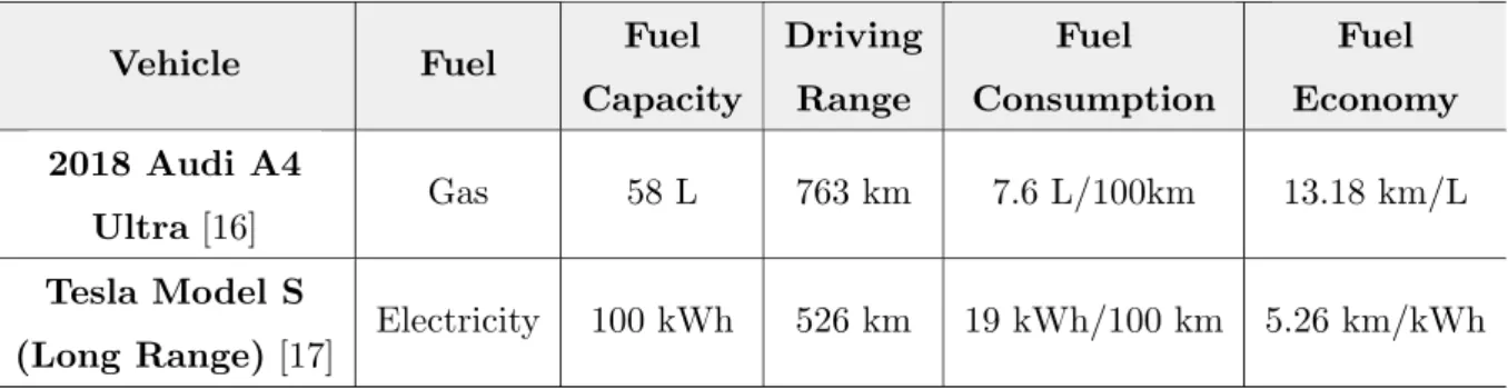
Table 2.1 shows some specifications of the fuel efficiency of two different types of vehicles, one ordinary internal combustion engine vehicle and one electric vehicle. The Tesla Model S (Long Range) has the largest driving range of all electric vehicles on the market today. As a consequence, electric vehicles are still way behind in terms of driving range.

Vehicle Fuel Fuel

Capacity Driving Range Fuel Consumption Fuel Economy 2018 Audi A4 Ultra[16] Gas 58 L 763 km 7.6 L/100km 13.18 km/L Tesla Model S

(Long Range) [17] Electricity 100 kWh 526 km 19 kWh/100 km 5.26 km/kWh

Table 2.1: Comparison of fuel consumption and fuel economy between an ordinary gas-powered car and an electric vehicle.

Power and Driving Range Reduction Analysis

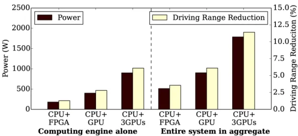
Every additional 1 kW consumed power decreases the fuel economy with about 1 km/L on average in a gas-powered car [18]. For example, in a 2018 Audi A4 Ultra, the fuel economy equals approximately 13.18 km/L (see Table 2.1) [16]. Hence, every additional 1 kW power consumption reduces the driving range with about 7.59%. In the left part of Figure 2.1, the impact of the power consumption on the driving range can be observed for different computing platforms.

However, most HAVs are most likely going to be electric vehicles. Due to the already much smaller driving ranges of electric vehicles, it is even more important to maintain an as low as possible total power consumption during autonomous driving. The energy consumption in electric vehicles is often expressed in kWh/100km, equivalent to the fuel consumption in gas-powered cars. Meaning that, the faster the vehicle travels, the more energy the system consumes. The Tesla Model S has a battery capacity of 100 kWh and a fuel consumption of 19 kWh/100km,

(29)

Figure 2.1: Power consumption and driving range reduction of the Audi A4 Ultra incorporating different computing platforms. On the left, only the computing platform is observed. On the right, the computing platform is observed in addition with the storage and cooling system, almost doubling the driving range reduction. Source [12]

resulting in a maximum driving range of 526 km (see Table 2.1). The national average traffic speeds in Europe vary from 34 km/h to 58 km/h [19]. Travelling at an average traffic speed of 45 km/h results in a power consumption of 45km_h ×19 kW h

100km = 8.55 kW. Finally, every additional

1 kW consumed power thus reduces the driving range with approximately 11.7%. The driving range reduction of the Tesla Model S is significantly higher than that of the Audi A4 Ultra, even though electric vehicles already suffer from smaller driving ranges. As a consequence, an electric vehicle suffers even more from a high additional power consumption.

Unfortunately, the additional consumed power brings a lot of additional heat with it. A cooling system is thus needed to control the temperature inside the vehicle such that the passengers feel no discomfort. The additional energy consumed by the cooling system is higher than one may expect. According to Joudi et al. [20], an automotive air conditioning system has a coefficient of performance of 1.3, representing the ratio of the amount of dissipated heat to the amount of work required to dissipate this heat. The inverse of this ratio is especially useful as it indicates a 77% of additional work is needed to dissipate the original heat. Hence, the additional energy required to cool the computing platform almost doubles the energy consumed by the computing platform alone.

The complete additional energy produced by an HAV compared to an ordinary vehicle consists of the energy generated by the computing platform, the data storage and the cooling system. The experiments in this dissertation mostly focus on the energy consumed by the computing platform alone. Now in the right part of Figure 2.1, Lin et al. [12] expressed the total power consumption of the ADS. It includes the energy consumed by the cooling system and storage

(30)

Autonomous Driving Architecture Overview 12

system. The total driving range reduction is almost doubled when compared to the driving range reduction imposed by the computing platform alone.

Power Consumption of Future Specialised Computing Platforms

Modern ADSs consist of multiple processing units, still consuming tremendous amounts of en-ergy. It is absolutely not absurd for affordable computing platforms of modern ADSs to produce 1 kW or more. However, more and more chip manufacturers are creating specialised chips for autonomous driving. These chips often consume much less power. For example, Nvidia’s state-of-the-art Drive AGX Orin processor only coming out in 2022 will consume around 70 W and will probably be part of a computing package such as its predecessor (Drive PX Pegasus consist-ing of two Drive PX Xavier processors and two Graphical Processconsist-ing Units (GPUs) consumconsist-ing 500 W [21]) such that the total still unknown power consumption of the computing platform will be approximately 750 W [22]. However, according to Liu et al., a leading autonomous driving company of which the name is withheld by request still uses an ADS with a peak power consumption of 5000 W [23]. It is thus of utmost importance to start reducing the power con-sumption during autonomous driving in order to maintain an as large as possible driving range.

2.3 Autonomous Driving Architecture Overview

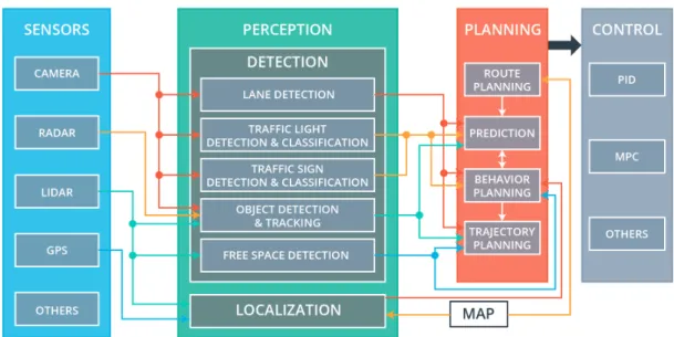
In this section, a short overview is given of the main tasks in autonomous driving which need to be performed continuously in an HAV [12, 23, 24, 25]. Later in this chapter, every task is explained in more detail. The main tasks and their relations can be visualised in Figure 2.2.

Figure 2.2: The figure shows a typical autonomous driving architecture, a modular autonomous driving pipeline divided in four main autonomous driving tasks: Sensing, Perception, Planning and Control. Source [25]

(31)

Autonomous Driving Architecture Overview 13

2.3.1 Sensing

The first step in autonomous driving is sensing the environment using different sensors for autonomous driving. The sensor data is then fed to the processing platform. HAVs operate under highly variable circumstances (different weather conditions, different road networks, different road users, etc.) and should be able to perform many different tasks (e.g., travelling in an urban environment, travelling on a highway, parking, etc.). Choosing an appropriate sensor suite is thus a very important part of designing an HAV. In the next section a broad overview is given of appropriate sensors for ADSs.

2.3.2 Perception

Once the sensor data is received by the processing platform, the processing platform will create a perception of the environment using the received sensor data. The processing platform is thus responsible for translating raw sensor data into an understandable data format for the ADS. This understandable data is a digital representation of the environment. Multiple different algorithms are needed to create such a digital perception of the environment. Every industry player has its own method to create this representation. Some industry players keep the representations of each perception task separated, whereas other industry players such as Waymo make use of the so-called HD Maps (see Section 2.5.3).

The following three primary perception subtasks can be distinguished:

• Object detection is responsible for identifying objects in the neighbourhood such as pedestrians, vehicles, road signs, traffic lights and lanes.

• Object tracking is responsible for tracking the motion of dynamic objects such as other cars and pedestrians.

• Localisation is the task of finding the position of the own vehicle (further referred to as the ego-vehicle).

These three perception subtasks contribute the most to the total power consumption of an ADS. They are explained more in depth in Section 2.5.

2.3.3 Planning

In the planning task, important decisions are taken in order to safely navigate the HAV from point to point. Both long-term and short-term decisions need to be made. The planning task primarily consists of mission planning and motion planning. Mission/Route planning is respon-sible for the long-term decisions while motion planning is responrespon-sible for short-term planning

(32)

Sensors 14

such as lane changing and obstacle avoidance. After the planning decisions have been made, the processing platform in the ADS sends the trajectory to the controller subsystem.

2.3.4 Control

Once the control subsystem receives the trajectory that the HAV should follow, the controller needs to calculate the necessary vehicle control commands and send them to the actuator sub-system. Finally, the actuator subsystem receives the actual driving commands such as breaking, accelerating and steering, and turns them into vehicle motions. The goal of the controller is to minimise the error or the deviation from the planned path. Different control methods could be used such as Model Predictive Control (MPC) and Proportional Integral Derivative (PID) control. HAVs need at least two different controllers:

• Longitudinal controller calculates the needed throttle percentage and break percentage. • Latitudinal controller is used to calculate the required steering angle.

2.4 Sensors

As already mentioned in the previous sections, choosing an appropriate sensor suite is a very important task in the design of an ADS. Different types of sensors are needed to overcome the high variability HAVs operate under as some sensors perform better than others under certain circumstances. The diversity of the sensors is not the only requirement for the sensors in an ADS. There also needs to be redundancy, for instance when one sensor fails, another should be able to replace it. HAVs should thus be equipped with a large number of sensors and both the positions and types of sensors need to be chosen wisely [26, 27, 28, 29, 30]. In Figure 2.3, a vehicle is shown with its corresponding sensors.

Two different types of sensors are distuingished: exteroceptive and proprioceptive sensors. Exteroceptive sensors measure values from the HAV’s environment.

• Light Detection and Ranging (LIDAR) is a technology to calculate the distance to an object using laser beams. It is used in HAVs to generate point clouds mapping the 3D environment. LIDAR sensors are a good fit for HAVs because of their very high accuracy and they often have a field of view of 360 degrees. On the contrary, LIDAR sensors do not have a high reliability as they are affected by poor weather conditions. For example, rain droplets can affect LIDAR’s accuracy due to the ability to perceive tiny objects. In addition, LIDAR sensors are sensitive to external light sources as light

(33)

Sensors 15

Figure 2.3: Typical sensors in an HAV with their corresponding functionality. Source [27]

beams are used to calculate the distances. On top of that, LIDAR sensors suited for autonomous driving are extremely expensive and drastically increase the total cost of an HAV. The cost of a single LIDAR sensor intended for autonomous driving can go up to about AC 70,000 (for instance, the Velodyne HDL-64E used in Waymo’s first self-driving cars). Lately a new LIDAR technology is emerging, Solid State LIDAR. It is LIDAR’s little brother and it is much cheaper, smaller and more durable as there are no moving parts [31]. The fact that Solid State LIDAR is completely static is both advantageous as disadvantageous because Solid State LIDAR is not able to capture such a wide field of view. Unfortunately, this technology is still largely being researched and tested for autonomous driving capabilities, however more and more companies are starting to sell this new technology, such as Blickfeld, Velodyne and XenomatiX.

• Radio Detection and Ranging (RADAR) sensors calculate the distances to objects using electromagnetic pulses or radio waves. The reason why RADAR sensors are widely used in HAVs is because they are a much cheaper option than LIDAR. As a result, RADAR sensors can be used in an ADSs to add a lot of necessary redundancy to the HAV, as can be seen in Figure 2.3. LIDAR is able to detect small and large objects, whereas RADAR is only able to detect larger objects, making RADAR sensors perform better under poor weather conditions. However, RADAR performs better under various different lighting conditions as well because radio waves are unaffected by light sources. In addition, radio waves can travel much further than light waves and sound waves making RADAR a perfect

(34)

Sensors 16

fit for ACC-like applications [29].

• Sound Navigation and Ranging (SONAR) is a technique used to calculate the dis-tances to objects using ultrasonic sound waves. While both RADAR and LIDAR can be used for short and long range distances, SONAR is mainly used for short ranges. Like RADAR, SONAR is rather inexpensive when compared to LIDAR and is unaffected by lighting and poor weather conditions. A great example of an application in autonomous driving where SONAR is used is automated parking.

• Camera sensor is used to create 2D images or even videos from the scene. Depending on the needed information, different vision-based algorithms can be performed on the images to get an estimate of the environment (for example, object detection algorithms such as road sign detection). Like LIDAR, cameras are sensitive to unfavourable weather conditions resulting in less reliability. Cameras are fairly inexpensive and have a rather wide field of view.

• Stereo camera is a camera with at least two lenses oriented in the same direction but from a different origin. Because the environment is captured from two different point of views, the proximity to objects in the field of view can be calculated. Stereo cameras are mainly used in HAVs as a low-cost alternative for the extremely expensive LIDAR sensors [32]. Unfortunately, like the ordinary camera sensors, stereo cameras are highly affected by unfavourable weather conditions.

Proprioceptive sensors measure values internal to the system or HAV.

• Global Navigation Satellite System (GNSS) is a navigation system with global cov-erage. The navigation system uses satellites to transmit radio waves to small electronic receivers in order to determine their location with meter-level precision [30, 33]. GNSSs are widely used in ordinary and self-driving vehicles to get a raw estimate of the ego-vehicle’s location. Examples of GNSSs include Galileo, GPS, GLObal NAvigation Satellite System (GLONASS) and BeiDou Navigation Satellite System (BDS).

• Inertial Measurement Unit (IMU) is a technology measuring the accelerations and angular velocities along its x, y and z-axes using a combination of accelerometers and gyroscopes. An IMU is often used in combination with a GNSS in order to provide a more precise representation of the ego-vehicle’s state (position, heading and velocity) [30]. • Rotary encoders are used to track the orientation of the wheels of a robot. This

(35)

Perception 17

used in robots to calculate the distance travelled from one point to another by tracking the speed of the wheels. It can also be used to calculate the speed and the orientation of the vehicle. Wheel odometry is highly susceptible to errors for example due to slipping. However, it is again mostly used in conjunction with other techniques to refine the position and orientation estimates [30].

2.5 Perception

In Figure 2.2, two main perception tasks can be observed, the detection task and the localisation task. In the figure, the detection task consists of five more detection subtasks which can actually just be categorised as two subtasks: object detection and object tracking. This simplification of the architecture is justified because there is a lot of similarity between the detection subtasks, most of them can be accomplished using the same algorithm and it greatly eases the research in this thesis. The new object detection subtask will perform the lane detection, traffic light detection & classification, traffic sign detection & classification, object detection and free space detection. The object tracking subtask becomes its own new subtask. As already mentioned in Section 2.3.2, the perception task thus consists out of three tasks: object detection, object tracking and localisation. Each of these three perception tasks plays a significant role in creating a perception of the environment.

2.5.1 Object Detection

The video stream is fed to the object detection task where all the important objects are detected, both static and dynamic objects (for example, pedestrians, vehicles, lanes, traffic signs, traffic lights, road barriers, etc.). It is important that next to the detection of the objects, the objects can also easily be classified. Every object has its own behaviour and when the objects are classified, the ADS has much more information to rely on and can much easier predict the behaviour of a specific object. For example, whenever a pedestrian is detected and classified, the ADS can already predict some motion in the upcoming frames.

Object detection and classification is most easily done using camera sensor data or vision data. LIDAR, RADAR and SONAR could be used to detect objects as well, however it is harder to classify the detected objects. In this dissertation, a state-of-the-art real-time vision object detection algorithm is used, namely You Only Look Once v3 (YOLOv3) [34]. It is capable of detecting and classifying a wide range of objects including vehicles, pedestrians, bicycles, traffic signs and traffic lights.