No growth in total global
CO
2
emissions in 2009
No growth in total global CO2 emissions in 2009
© Netherlands Environmental Assessment Agency (PBL), Bilthoven, The Netherlands, June 2010
PBL publication number 500212001
Corresponding author: Jos Olivier; jos.olivier@pbl.nl
Parts of this publication may be reproduced, providing the source is stated, in the form: Netherlands Environmental Assessment Agency, June 2010, No growth in total global CO2 emissions in 2009
This publication can be downloaded from our website: www.pbl.nl/en.
The Netherlands Environmental Assessment Agency (PBL) is the national institute for strategic policy analysis in the field of environment, nature and spatial planning. We contribute to improving the quality of political and administrative decision-making by conducting outlook studies, analyses and evaluations in which an integrated approach is considered paramount. Policy relevance is the prime concern in all our studies. We conduct solicited and unsolicited research that is both independent and always scientifically sound.
Netherlands Environmental Assessment Agency
Office The Hague Office Bilthoven
PO Box 30314 PO Box 303
2500 GH The Hague 3720 AH Bilthoven
The Netherlands The Netherlands
Telephone: +31 (0)70 328 8700 Telephone: +31 (0)30 274 2745 Fax: +31 (0)70 328 8799 Fax: +31 (0)30 274 4479 E-mail: info@pbl.nl
No growth in total CO2 emissions in 2009
Abstract
In 2009, for the first time since 1992, there was no growth in global carbon dioxide (CO2) emissions from fossil fuel use, cement production and chemicals production. The recent credit crunch drove many industrialised economies into recession, particularly OECD countries and Russia, and led to a dramatic decrease in CO2 emissions of 7% in 2009 in these countries. This drop of 800 million tonnes in emissions has compensated for the continued strong increase in CO2 emissions in China and India of 9 and 6%, respectively. In the same year, emissions in other developing countries did not vary as much. These preliminary estimates have been made by the Netherlands Environmental Assessment Agency (PBL) on the basis of energy data for 2008 and 2009 recently published by BP (British Petroleum) and the International Energy Agency (IEA). The estimates are also based on production data on cement, ammonia and steel and emissions per country from 1970 to 2005 from the joint EDGAR project of the European Commission’s Joint Research Centre (JRC) and the Netherlands Environmental Assessment Agency (PBL).
1. Introduction
This paper discusses the method and results of a trend assessment of global CO2 emissions up to 2009 and updates last year’s assessment up to and including 2008. The current assessment includes not only fossil fuel combustion on which the BP reports are based, but also incorporates all other relevant CO2 emissions sources including flaring of waste gas during oil production, cement clinker production and other limestone uses, feedstock and other non-energy uses of fuels, and from several other small sources.
The assessment excludes CO2 emissions from deforestation and logging, forest and peat fires, from post-burn decay of remaining above-ground biomass, and from decomposition of organic carbon in drained peat soils. The latter mostly affects developing countries. These sources could add as
much as a further 20% to global CO2 emissions. However, this percentage is highly uncertain and varies widely between years. This variation is also a reason that emissions and sinks from land use, land-use change and the forestry sector (LULUCF) are kept separate from the UN Climate Convention (UNFCCC) and the Kyoto Protocol. For the same reason, the emissions from the LULUCF sector are not included in this assessment. Information on recent emissions from forest and peat fires and post-burn emissions is being assessed by the Global Carbon Project, which will publish later this year a comprehensive assessment of the global carbon budget including all sources and sinks (GCP, 2010).
The estimate of global CO2 emissions from 1970 to 2005 is based on the results of the EDGAR 4.1 dataset, a joint project of the European Commission’s Joint Research Centre (JRC) and the Netherlands Environmental Assessment Agency (PBL). This dataset provides greenhouse gas emissions per country and on a 0.1 x 0.1 degree grid for all anthropogenic sources identified by the IPCC for the period 1970-2005 (JRC/PBL, 2010). Although the publicly released dataset distinguishes about 25 sources categories, emissions are estimated for well over 100 detailed categories as identified in the Revised 1996 IPCC guidelines for compilation of emission inventories (IPCC, 1996).
For fuel-related combustion emissions, the EDGAR dataset uses detailed international energy statistics from the International Energy Agency (IEA, 2009) and the latest methodology, and CO2 emission factors for 56 fuel types published in the 2006 IPCC Guidelines for GHG Emission Inventories (IPCC, 2006). Other sources of CO2 emissions included are flaring and venting of associated gas from oil production, the production of minerals such as cement and lime, metals production, the production of chemicals such as ammonia and ethylene, and several other small sources such as lubricant and wax use. Moreover, to improve completeness, several other small sources identified in the 2006 IPCC Guidelines were added, such as waste incineration
No growth in total global CO
2
emissions in 2009
CO
2
from fossil fuels and cement in China and India jumps
(6C) and underground coal fires in China and elsewhere (7A). These sources add about 0.3% to fuel combustion emissions. The EDGAR 4.1 dataset also includes annual CO2 emissions from forest fires and peat fires as well as fires in savannahs and other wooded land estimated by Van der Werf et al. (2006). Their study uses the GFED model that uses high resolution satellite observations of burned areas, land use maps and a model to estimate carbon density per grid cell and the fraction of carbon burnt1. EDGAR 4.1 also includes the significant, albeit highly uncertain, CO2 emissions from the decay of organic materials of plants and trees, which remain after forest burning and logging, and from drained peat soils (JRC/PBL, 2010).
For this assessment, the EDGAR 4.1 dataset was used which differs from the basic historical data in EDGAR 4.0 used last year. EDGAR 4.1 includes the latest CO2 emission factors for cement production (e.g., kg CO2/ton cement produced). In addition, all sources of CO2 related to non-energy/feedstock uses of fossil fuels were estimated using the tier 1 methods and data recommended in 2006 IPCC Guidelines on GHG Inventories (IPCC, 2006)2. As well as cement production, EDGAR 4.1 includes other industrial non-combustion processes such as production of lime and soda ash (2A) and carbon used in metal production (2C). Collectively, these sources add 21% to global cement production emissions in 2005.
2. Methodology and data sources for the 2006-2009
period
For the trend estimate for the period 2005-2009, all CO2 emissions were aggregated into the following main source sectors (corresponding IPCC category codes in brackets): fossil fuel combustion (IPCC categories 1A, including
international transport ‘bunkers’, marine and aviation); fugitive emissions from fuels (IPCC category 1B); cement production and other carbonate uses (IPCC
category 2A);
feedstock and other non-energy uses of fossil fuels (IPCC categories 2B+2C+2G+3+4D4);
waste incineration and fuel fires (IPCC categories 6C+7A). For each country, the trend from 2005 onwards was estimated using the appropriate activity data or
1 Annual CO2emissions from forest and peat fires from 1997 to 2009
have been estimated by Van der Werf et al. (2010) using the GFED 3.1 model. Their analysis does not include CO2 emissions from the decay of
organic materials of plants and trees after burning and logging.
2 Up until 2008, the IEA dataset was used which calculates CO2 emissions
using the amounts of fuels used for non-energy purposes such as activity data and an aggregate global oxidation factor per fuel type as emission factor. This change in method and source allocations leads to approxi-mately the same total global CO2 emissions in the non-energy/feedstock
source categories for the years since 1980 (-4% difference, on average). However the differences can be much larger for individual countries. Before 1980, the global totals of two datasets diverged, with differences increasing from 15% in 1979 to 45% in 1970. The IEA shows much lower emissions probably due to less separation in the reporting of non-energy and feedstock uses.
approximated with trends in related statistics as estimator. For the large fraction of fuel combustion emissions (1A) that account for about 90% of total global CO2 emissions excluding forest fires, 2005 emissions were divided per country into four main fuel types for use as trend indicators. These fuel types are coal and coal products, oil products, natural gas and other fuels (e.g., fossil-carbon containing waste oils). For each fuel type, the 2005-2007 trend was based on IEA data released in 2009 (IEA, 2009), and the 2007-2009 trend on BP data released in June 2010 (BP, 2010).
Likewise, the fugitive emissions from fuels (1B) were divided into solid fuels (coke production), and oil and gas (gas flaring and venting). Minerals production (2A) was divided into cement production and other sources, and for the latter, lime production was used as trend indicator. For other non-fuel combustion sources, for chemicals production (2B) – including liming of soils with urea (4D4) – ammonia was used as trend indictor, and for metal production (2B), crude steel production was used. For the other small non-energy uses of lubricants, waxes and solvents (2G+3), the past trend was extrapolated. The same was done for category 7A that comprises the relatively small underground coal fires3 and oil and gas fires (in Kuwait in 1992).
More details on the methodology and data sources are presented in Annex 1. Data quality and uncertainty in the data are also briefly discussed in this Annex. The uncertainty in CO2 emissions from fossil fuel combustion using international statistics is discussed in detail by Marland et al. (1999) and general uncertainty characteristics in global and national emission inventories in Olivier and Peters (2002).
3. Results
3.1 Essentially no growth in global CO2 emissions in 2009
After correction for the leap year 2008 and accounting for uncertainties in the data, total global emissions have essentially stabilised in 2009. Although arithmetically global emissions decreased slightly (-0.7% with leap year correction), the uncertainties estimated in the country trends and particularly in the difference of regions with growing and with decreasing emissions are such that we must conclude that the emissions have essentially stabilised in 2009. This compares with the six years since 2002 with average annual growth rates of 3.5%. In 2008, when the impacts of the credit crunch became visible, global emissions increased by about 1.5%. This is the first time since the 1992 recession that global CO2 emissions have not increased. Previous recessions due to large increases in oil price led to global decreases in CO2 emissions in 1974-1975 and 1980-1982. In October 2009, the International Energy Agency (IEA) expected that global CO2 emissions would decrease by 2.6% in 2009 (Reuters, 2009). This would have been the largest drop in more than 40 years because the global recession froze economic activity and slashed energy use around the world.
3 Underground coal fires are mainly in China and India. The global total is estimated in EDGAR 4.1 at about 46 million tonnes, of which about two-thirds originates from China, with a high uncertainty of about 50%.
No growth in total CO2 emissions in 2009 However, the growth pattern has been sustained in China
and India. This conclusion is based on EDGAR estimates for 1970 to 2005, IEA trends for 2006 and 2007, BP data 2007 to 2009, and other trends. This sustained growth has occurred regardless of the credit crunch that has affected most industrialised countries and is largely compensated for by the decreases calculated for the industrialised countries that have emission mitigation targets under the Kyoto Protocol. 3.2 Large regional differences: China and India jump by
9% and 6% while OECD countries plummet by 7% The recession in OECD-19904 countries has led to large drops in output of heavy, energy-intensive industries such as steel and basic chemicals production, oil refineries and power generation. In Europe, CO2 emissions from industries regulated by the Emissions Trading Scheme fell by 11.6% (Reuters, 2010a) and in the USA, industry emissions from fuel combustion fell by 11% and power generation by 9% (EIA, 2010). Total emissions in the European Union (EU-15) fell by 7% to 3.1 billion tonnes and in the USA by 7% to 5.3 billion tonnes. The total CO2 emissions in Japan and Russia fell by 11% to 1.2 billion tonnes and 9% to 1.6 billion tonnes, respectively. Total CO2 emissions fell by 7% in all industrialised countries with quantitative greenhouse gas mitigation targets under the Kyoto Protocol.
China and India
Since 2000, CO2 emissions in China have more than doubled, and in India have increased by more than half. Since the end of 2008, China, has been implementing a large economic stimulus package over a two-year period. This package includes investment in transport infrastructure and in rebuilding Sichuan communities devastated by the 2008 earthquake. In 2009, CO2 emissions jumped by 9% to 8.1 billion tonnes, even though China has doubled its installed wind and solar power capacity for the fifth year in a row. India where domestic demand makes up three-quarters of the national economy is relatively unaffected by the credit crunch.
4 Here we use the composition of the OECD in 1990 (without Mexico, Korea, Czech Republic, Slovakia, Hungary and Poland).
Emissions continued to increase in 2009 by 6% to 1.7 billion tonnes of CO2. India has now surpassed Russia as the fifth largest CO2 emitter (Figure 3.2).
Other developing countries
The picture is more diffuse in other developing countries, ranging from countries with increasing emissions such as Iran, Indonesia and South Korea, to those with decreasing emissions, such as Brazil, Saudi Arabia, South Africa and Taiwan. In total, CO2 emissions in these countries changed very little in 2009.
Global emissions
In 2009, total global CO2 emissions had increased 25% since 2000 to 31.3 billion tonnes and almost 40% since 1990, the base year of the Kyoto Protocol. In 1990, global emissions were 22.5 billion tonnes, an increase of 45% on the 1970 level of 15.5 billion tonnes. The very large regional variation in emission trends in 2009 resulted in a 53% share of developing countries versus 44% for industrialised countries with mitigation target for total greenhouse gas emissions under the Kyoto protocol. The remaining 3% is accounted for international air and sea transport. The top-6 emitting countries, including the EU-15, comprise two-thirds of total global emissions whereas the top-25 emitting countries capture more than 80% of total emissions (Figure 3.2). Emissions per capita
While emissions in China and other developing countries have increased rapidly in recent years, also in absolute figures, the picture is different for CO2 emissions per capita (Table 3.1 and Figure 3.3) or per unit of GDP (Figure 3.4). Since 1990, CO2 emissions per capita have increased in China from 2.2 to 6.1 tonne per capita and decreased in the EU-15 from 9.1 to 7.9 tonne per capita and from 19.5 to 17.2 tonne per capita in the USA. These changes reflect a number of factors including the large economic development in China, structural changes in national and global economies, and the impact of climate and energy policies. Due to rapid economic development, per capita emissions in China are quickly approaching levels common in the industrialised countries of the Annex I group
Global CO2 emissions from fossil fuel use and cement production, 1990-2009. Figure 3.1 1990 1995 2000 2005 2010 0 10 20 30
40 1000 million tonnes CO2 International transport
Developing countries
Other developing countries Other big developing countries China
Industrialised countries (Annex I) Other Economies In Transition (EIT) Russian Federation
Other OECD1990 countries Japan
EU-15 USA
Top-25 CO2-emitting countries in 2008 and 2009 Figure 3.2 China USA EU-15 India Russian Federation Japan Germany Iran South Korea Canada United Kingdom Mexico Indonesia Italy Australia Brazil South Africa Saudi Arabia France Spain Ukraine Poland Taiwan Thailand Netherlands 0 2000 4000 6000 8000 10000 million tonnes CO2
Industrialised countries (Annex I) 2008
2009 Developing countries
2008 2009
Top 25 of largest CO2-emitting countries in 2009
CO2 emissions in 2009 (million tonnes CO2) and trends in CO2/capita emissions 1990-2009 (unit: tonne CO2/person)
Country Emissions 2009 1990Per capita2000 emissions2008 2009 2000-2009Change percentageChange in
ANNEX I * United States * 5,310 19.5 20.5 18.6 17.2 -3.4 -16% EU-15 ** 3,050 9.1 8.8 8.5 7.9 -0.9 -11% - Germany 770 12.9 10.5 10.0 9.3 -1.2 -11% - United Kingdom 490 10.3 9.3 8.8 8.1 -1.3 -14% - Italy 410 7.5 7.9 7.6 7.0 -0.9 -12% - France 370 6.8 6.8 6.3 6.0 -0.8 -12% - Spain 310 5.8 7.5 8.0 7.1 -0.4 -6% - Netherlands 160 9.8 10.0 9.9 9.7 -0.3 -3% Russian Federation 1,570 15.7 10.8 12.2 11.2 0.4 3% Japan 1,180 9.4 10.0 10.3 9.2 -0.8 -8% Canada 540 16.2 18.0 17.5 16.3 -1.7 -9% Australia 400 16.2 18.7 19.2 18.8 0.1 1% Ukraine 310 20.1 9.1 9.3 8.0 -1.1 -12% Poland 280 6.1 5.6 6.3 6.2 0.6 11% NON ANNEX I China 8,060 2.2 2.8 5.6 6.1 3.2 113% India 1,670 0.8 1.0 1.4 1.4 0.4 38% Iran 570 3.6 5.2 7.5 7.7 2.5 48% South Korea 560 5.9 9.8 11.4 11.5 1.8 18% Mexico 470 3.7 3.8 4.2 4.2 0.3 8% Indonesia 440 0.9 1.4 1.9 1.9 0.5 36% Brazil 380 1.5 2.0 2.1 1.9 0.0 -1% South Africa 380 7.3 6.8 8.2 8.0 1.2 18% Saudi Arabia 370 9.8 11.8 14.4 13.6 1.9 16% Taiwan 260 6.3 10.1 11.4 10.7 0.6 6% Thailand 240 1.7 2.8 3.7 3.6 0.8 30%
* Annex I countries: industrialised countries with annual reporting obligations under the UN Framework Convention on Climate Change (UNFCCC) and emission targets under the Kyoto Protocol. The USA has signed but not ratified the protocol, and thus the emission target in the protocol for the USA has no legal status.
** EU 15 = 15 EU Member States at the time the Kyoto Protocol was ratified. Source of population data: UN WPP Revision 2004.
No growth in total CO2 emissions in 2009 under the Kyoto Protocol. In fact, present CO2 emissions per
person in China are now similar to France. 3.3 Trends in fossil fuel consumption
Fossil fuel combustion accounts for about 90% of total global CO2 emissions excluding forest fires (EDGAR 4.1, JRC/PBL, 2010). BP (2010) states that global oil consumption emissions fell by about 1.7% in 2009, which is the largest decline since 1982 (including leap day correction for 2008). Here too is a divergence between OECD and non-OECD countries of 4% decrease versus a 2% increase, respectively, with the growth occurring in China, India and the Middle Eastern countries. Natural gas consumption fell globally by 2.1%, the largest decline on record. Consumption in OECD countries fell by 3%, mainly due to the recession which also affected the basic chemicals industry. Russia saw the largest decline of 6%, even with the colder winter months than in 2008 (see Annex 3 for the regional impact on the trend of winter temperatures in 2008 and 2009).
Coal consumption was essentially constant but with large differences per region. Consumption in OECD countries and former Soviet Union plummeted by 10 and 13% respectively, the steepest declines on record. According to BP (2010), this is due to the recession that has had a large impact on steel production and power generation which rely heavily on coal. Elsewhere, coal consumption increased by 7%, with China accounting for 95% of the increase, according to BP (2010). 3.4 Trends in non-energy sources
Despite the worldwide recession, global cement production increased by 8% in 2009 with resulting CO2 emissions from the limestone use in clinker production increasing by 7% as this clinker fraction in cement continues to decrease. Production is estimated to have decreased in all but seven countries (USGS, 2010; China Weekly News, 2010). The notable exceptions are China (+17%), Pakistan and Russia (+3%), and Brazil and India (+2%)
A study by the World Business Council on Sustainable Development (WBCSD, 2009) has shown that in recent years the cement industry in most countries has considerably increased the share of blended cement compared to the traditional Portland cement. This change has resulted in average clinker fractions in total cement production of between 70 and 80% compared to around 95% in Portland cement.
Both non-combustion and combustion emissions from cement production relate specifically to the clinker
production process and not to mixing of cement clinker. This has resulted in about 20% decrease in CO2 emissions per tonne of cement produced compared to the 1980s. At that time, it was not common practice to blend cement clinker with other mixing materials, such as fly ash from coal-fired power plants or blast furnace slag. According to EDGAR 4.1 data, this has resulted in an annual decrease of 250 million tonnes in CO2 emissions compared to the reference case of Portland cement production (JRC/PBL, 2009, 2010). Moreover, a similar amount has been reduced in fuel combustion emissions from cement production.
According to WSA (2010), global production of crude steel fell by 8% in 2009, with decreases in all countries except China (+13%), Iran (+9%) and India (+3%). Lime production fell globally by 5%, and ammonia production was estimated to be flat (USGS, 2010).
3.5 Trends in renewable energy sources
The trends in CO2 emissions include the impact of policies to improve energy efficiency and to increase the share of renewable energy sources over that of fossil fuels. Wind power capacity in the world grew 31% in 2009 (GWEC, 2010), with one-third of new installations in China. For the fifth year in a row, China has doubled its installed wind power capacity. Total solar photovoltaic power installed in 2009 is 46% up on 2008, with 70% installed in Europe which is about 50% more than in 2008 (EPIA, 2010). The USA also installed 50% more in 2009 and China doubled its installed capacity.
China now leads the world in large-scale hydropower with 19% of global production, and is well before Brazil and the USA with a 12% share each.
The annual increase in biofuel use in road transport of 15% in 2009 was lower than in previous years which saw about 30% increase (Annex 2). The increase in Brazil and the USA in 2009 was 17% and 12% respectively, whereas Germany saw a 2% decrease. Present fuel ethanol and biodiesel use represents about 3% of global road transport fuels, and would have reduced CO2 emissions by a similar percentage if all biofuel had been produced sustainably. In practice, however, net reduction in total emissions in the biofuel production and consumption chain is between 35% and 80% (Eijkhout et al., 2008; Edwards et al., 2008). These estimates also exclude indirect emissions such as additional deforestation (Ros et al., 2010). An example of the latter is biodiesel produced from palm oil from plantations on deforested and partly drained peat soils. Thus, the effective reduction will be between 1 and 2% excluding possible indirect effects.
4. Consequences for the Kyoto Protocol
targets and emission trading
Collectively, the Annex I countries to the Kyoto Protocol reduced CO2 emissions in 2009 by about 7%. Assuming that the non-CO2 greenhouse gas emissions show a similar trend, the total 2009 emissions of the Annex I countries are about 10% lower than in 1990, the base year for the protocol. The decreases in 2008 and 2009 will help industrialised nations to meet their target under the Kyoto Protocol. Except for the United States, these countries are due to cut emissions collectively by an average of at least 5.2% below 1990 levels by 2008-2012. However, since a large part of the decreases is due to a freeze or drop in economic activity in response to the credit crisis, greenhouse gas emissions could rapidly increase toward pre-recession levels as industrialised countries grow out of recession. Most of the industry capacity is still in place and the idle part is waiting to start producing again. In past recessions due to bank crises or oil price shocks, it took about 2 to 4 years after the dip for energy
consumption and CO2 emissions to recover at pre-recession levels, if at all.
A consequence of the large decrease in Annex I emissions in the Kyoto target period 2008-2012 is that less emission credits from certified emission reduction projects under the UN Clean
CO2 emissions per capita in 1990 and 2009 in the top-25 CO2-emitting countries. Figure 3.3 Australia USA Canada Saudi Arabia South Korea Russian Federation Taiwan Netherlands Germany Japan United Kingdom South Africa EU-15 Iran Ukraine Spain Italy Poland China France Mexico Thailand Brazil Indonesia India 0 4 8 12 16 20 tonne CO2 / capita
Industrialised countries (Annex I) 1990
2009 Developing countries
1990 2009
CO2 emissions per capita
CO2 emissions per unit of GDP in 1990 and 2009 in the top-25 CO2-emitting countries (source of GDP data: IMF, 2010) Figure 3.4 Ukraine China South Africa Russian Federation Iran Saudi Arabia India Australia Indonesia Thailand Canada South Korea Poland USA Taiwan Mexico Japan Germany Netherlands EU-15 Italy Spain United Kingdom Brazil France 0 500 1000 1500 2000
tonne CO2 / USD2005 (PPP-adjusted)
Industrialised countries (Annex I) 1990 2009 Developing countries 1990 2009 CO2 emissions per GDP
No growth in total CO2 emissions in 2009 Development Mechanism (CDM) will be purchased to meet
national Kyoto targets.
The same applies to companies registered under the European Emission Trading Scheme. The UN Environment Programme Risø centre estimates that less funds will flow to developing countries where these projects are being implemented (Reuters, 2010b). Risø’s present projection is that around 1.0 billion tonnes of Certified Emission Reductions (CER units) will come to the market by the end of 2012 when the Kyoto period expires. This estimate is about half that predicted by Risø three years ago. A total of 1 Tg CO2 reduction represents about 200 Tg CO2 per year in a five-year period, which is roughly equal to the annual CO2 emissions of the Netherlands.
However, individual countries such as Australia, Canada, New Zealand and Spain, may still need to purchase emission credits from other countries in order to meet their targets. These may be either CDM credits from developing countries or credits from other industrialised countries that have a large surplus compared to their target (Den Elzen et al., 2009).
Annex 1. Method for estimating CO
2emissions
trends for the period 2005-2009
A.1.1 Methodology and data sourcesThe recent trends were estimated by PBL using trends in most recent data on fossil fuel consumption for 2007-2009 from the BP Review of Energy 2009 (BP, 2010). For cement production, 2005-2009 data were used from the US Geological Survey (USGS) except for China for which use was made of China Weekly News (2010).
For the trend estimate 2005-2009, the following procedure was used. Sources were disaggregated into five main sectors as follows with the defining IPCC source category codes in brackets:
(1) fuel combustion (1A+international marine and aviation bunkers);
(2) fugitive emissions from fuels (1B);
(3) cement production and other carbonate uses (2A); (4) non-energy/feedstock uses of fuels
(2B+2C+2D+2G+3+4D4);
(5) other sources: waste incineration, underground coal fires and oil and gas fires (1992, in Kuwait) (6C+7A).
For these main source sectors the following data was used to estimate 2006-2009 emissions:
(1) Fuel combustion (IPCC category 1A+international bunkers): For energy for 2005-2007, the most recent detailed CO2
estimates compiled by the International Energy Agency (IEA) for fuel combustion by major fossil fuel type (coal, oil, gas, other) for these years (IEA, 2009) to calculate the trend per country and for international air and water transport.
For energy for 2007-2009, the BP Review of World Energy to calculate the trend of fuel consumption per main fossil fuel type: coal, oil, gas (BP, 2010).
For oil consumption, these figures were corrected for biofuel (fuel ethanol and biodiesel) which are included in the BP oil consumption data. See Annex 2 for more details. ‘Other fuels’, which are mainly fossil waste combusted
for energetic purposes, were assumed to be oil products and the trend was assumed to follow oil consumption per country.
For the trend in international transport, which uses only oil as a fuel, we applied the trend in total global oil consumption.
(2) Fugitive emissions from fuels (IPCC category 1B): Fugitive emissions from solid fuel (1B1), which for CO2
refers mainly to coke production: trends per country for 2005-2009 are assumed to be similar to the trend in crude steel production from the Word Steel Association (WSA, 2010).
Fugitive emissions from oil and gas (1B2), which refers to leakage, flaring and venting: trends per country for 2005-2008 are assumed to be similar to the trend in the top-20 of flaring from the World Bank’s Global Gas Flaring Reduction Programme (GGFR, 2010). 2008 data were extrapolated for 2009.
(3) Cement production and other carbonate uses (2A): cement production (2A1)
other carbonate uses, such as lime production and limestone use
soda ash production and use.
CO2 emissions from cement production, which amount to more than 90% of 2A category, were calculated using cement production data for 2006-2009 published by the US Geological Survey (USGS), except for China where use was made of China Weekly News (2010). In addition, we extrapolated the trend in the emission factor due to trends in the fraction of clinker in the cement produced based on data reported by WBCSD (2009). For all other sources in the minerals production category (2A), we used lime production data for 2006-2009 (USGS, 2010) as proxy to estimate the trend in the other 2A emissions. All 2009 data are preliminary estimates.
(3) Non-energy/feedstock uses of fuels (2B+2C+2D+2G+3+4D4):
ammonia production (2B1): net emissions, i.e. accounting for temporary storage in domestic urea production (for urea application see below);
other chemicals production, such as ethylene, carbon black, carbides (2B other);
blast furnace (2C1): net losses in blast furnaces in the steel industry, i.e. subtracting the carbon stored in the blast furnace gas produced from the gross emissions related to the carbon inputs (e.g., coke and coal) in the blast furnace as a reducing agent, since the CO2 emissions from blast furnace gas combustion are accounted for in the fuel combustion sector (1A);
another source in metal production is anode consumption (e.g., in electric arc furnaces for secondary steel
production, primary aluminium and magnesium production) (2C);
consumption of lubricants and paraffin waxes (2G), and indirect CO2 emissions related to NMVOC emissions from solvent use (3);
urea applied as fertiliser (4D4), in which the carbon stored is emitted as CO2 (including emissions from limestone/ dolomite used for liming of soils).
For the feedstock use for chemicals production (2B), ammonia production from USGS (2010) was used (2009 data are preliminary estimates). Since CO2 emissions from blast furnaces are by far the largest subcategory within the metal production category 2C, the trend in crude steel production from Word Steel Association (WSA, 2010) was used to estimate the recent trend in the total emissions. For the very small emissions in categories 2G and 3, the 2000-2005 trend was extrapolated. For simplicity, it was assumed that the small soil liming (4D4) emissions follow the gross ammonia production trend.
(5) Other sources (6C+7A):
waste incineration (fossil part) (6C) fossil fuel fires (7A).
The 2000-2005 trend was extrapolated for the relatively very small emissions of waste incineration (6C) and underground
No growth in total CO2 emissions in 2009 coal fires (mainly in China and India) and oil and gas fires
(1992, in Kuwait) (7A).
CO2 emissions from underground coal fires in China and elsewhere have been included in EDGAR 4.0, although the magnitude of these sources is very uncertain. The estimates for the amount burned in China varied by a factor of 10. However, new analysis of available information by Van Dijk et al. (2009) has shown that the higher number referred to the amount ‘lost’, which includes all coal below the fire area that has been made inaccessible because of the fire. This would be a factor of 10 higher than the amount of coal burned. Their conclusion is that emissions from coal fires in China are at the lower end of the wide range of 15-45 and 150-450 Tg per year, thus around 30 Tg CO2 per year. This is equivalent to about 0.4% of China’s CO2 emissions in 2009.
A.1.2 Differences between EDGAR version 4.1 and 4.0 The main changes in CO2 emissions between EDGAR version 4.0 and 4.1 is in cement production (IPCC code 2A1). This is due to the introduction of explicit accounting for the share of blended cement in total cement production and thus for the fraction of cement clinker in total cement production per country. It has resulted in 17% reduction in global CO2 emissions from cement production in 2005 (about 200 Tg). Another significant improvement is the removal of double counting in iron and steel production (2C) of about 2 Pg in 2005. This was already included in last year’s global trend analysis.
Small differences between version 4.1 and version 4.0 (used in 2008) are in the following source categories (IPCC source code in brackets):
gasworks and other transformation sector (1A1c) road transport (1A3b), urea production (2B5) non-energy use of lubricants and waxes (2G). New sources included in version 4.1 are:
chemicals production (2B): ammonia, ethylene and carbon black that account for 350 Tg CO2 in 2005
other metal production (2C): aluminium, lead and zinc that account for 70 Tg CO2 in 2005.
A.1.3 Other sources of CO2 emissions: forest
and peat fires and post-burn decay
The trend estimates of CO2 emissions do not include CO2 emissions from deforestation/logging and peat fires and subsequent post-burn emissions from decay of remaining above ground biomass and from drained peat soils. Although significant but highly uncertain, CO2 emissions from the decay of organic materials of plants and trees that remain after forest burning and logging are also not included. Annual CO2 emissions and from peat in Indonesia have been estimated at 400-5000 million tonnes CO2 (Hooijer et al., 2006), including emissions from drained peat soils. New estimates by Van der Werf et al. (2008) indicate that except for peak years due to an El Niňo, emissions from peat fires are not as large as the wide range suggests.
A.1.4 Data quality and uncertainties
For industrialised countries, total CO2 emissions per country from EDGAR 4.1 for the period 1990-2005 are generally
within 3% of officially reported emissions, except for a few economies in transition.
For recent years, trends in energy data published annually by BP appear to be reasonably accurate. For example, based on older BP energy data, the increase in 2005 in global CO2 emissions from fuel combustion was estimated at 3.3% globally. With presently available and more detailed statistics of the International Energy Agency (IEA) for 2005, the increase is estimated at 3.2%. At country level, differences can be larger, particularly for small countries and countries with a large share in international marine fuel consumption (bunkers) and with a large share in non-combustion fuel use. Moreover, energy statistics for fast changing economies, such as China, are less accurate than those for the traditional, industrialised countries within the OECD.
Other recent analyses of CO2 emissions from fossil fuel use and cement production have suggested that the uncertainty in CO2 emission estimates could be about 2 to 3% for the USA and as high as 15 to 20% for China (Gregg et al., 2008). However, this uncertainty in the estimate for China is based on revisions of energy data for the transition period in the late 1990s, which may not be applicable to more recent energy statistics. Based on subsequent revisions of emission estimates made by the IEA, PBL estimates the uncertainty in the preliminary estimates for China − caused by uncertainty in the energy data − at about 10%.
The uncertainty in CO2 emissions from fossil fuel combustion using international statistics is discussed in detail in Marland et al. (1999), and general uncertainty characteristics in global and national emission inventories in Olivier and Peters (2002). A.1.5 Results
Table A1.1 shows the trends in CO2 emissions per region/ country for 1990-2009 as presented in Figure 3.1. This table and the figures used in Figures 3.3 and 3.4 can also be found as spreadsheet on the PBL website:
http://www.compendiumvoordeleefomgeving.nl/indicatoren/ nl0533-Koolstofdioxide-emissie-door-gebruik-van-fossiele-brandstoffen%2C-mondiaal.html?i=9-20
Annex 2. Dataset on biofuel consumption
for transport per country, 2005-2009
This dataset is restricted to bioethanol or fuel ethanol and biodiesel used in transport as substitute for fossil oil products (petrol, diesel or LPG). Palm oil and solid biomass used in stationary combustion such as power generation was not considered, as it is not relevant for this study (see Table A2.1). Biofuel consumption data for road transport were used for 2005-2009 from the following sources:
CRF (2010) for Annex I countries (countries reporting emissions to the UN Climate Secretariat, at present data for 1990-2008), except for Bulgaria, Romania and the UK, that reported ‘Not Occuring’ or ‘Not Estimated’.
For European Union countries, these data were supplemented with fuel ethanol and biodiesel
consumption data for 2005-2008 from Systèmes solaires (2007, 2008, 2009) and EBB (2010), e.g. for Bulgaria, Romania and the UK.
Supplemental data for 2009 for the USA, Germany and Brazil, comprising almost 80% of the global total consumption were taken from EIA (2010b), BMU (2010) and Barros (2010), respectively.
For developing countries, various sources were used to obtain bioethanol and biodiesel consumption data for 2005-2008 in Brazil and Thailand. Consumption data were used for selected years for China, India and Argentina. Where time series were incomplete, amounts and trends were calculated using global trends of total bioethanol and biodiesel production 2000-2008 from the Renewables Global Status Report. 2009 Update (REN21, 2009). The global trend 2005-2009 for fuel ethanol production was taken from F.O. Licht cited by Global Renewable Fuels Alliance (GRFA, 2010) and for biodiesel from Renewable Energy Magazine (2010). Only data for 2005 onwards are presented here because correction for earlier years is not relevant for the CO2 estimation methodology used. This is only relevant for 2005/2006 onwards. For earlier years, the EDGAR 4.1 data are
Trends in CO2 emissions per region/country 1990-2009 (unit: billion metric tonnes of CO2)
1990 1991 1992 1993 1994 1995 1996 1997 1998 1999 2000 2001 2002 2003 2004 2005 2006 2007 2008 2009 USA 4.97 4.94 5.02 5.17 5.24 5.24 5.41 5.55 5.61 5.66 5.84 5.73 5.77 5.82 5.89 5.92 5.83 5.90 5.71 5.31 EU-15 3.32 3.36 3.27 3.22 3.22 3.26 3.34 3.27 3.31 3.29 3.32 3.39 3.38 3.46 3.46 3.42 3.41 3.36 3.28 3.05 - France 0.38 0.41 0.40 0.38 0.37 0.38 0.39 0.39 0.41 0.40 0.40 0.41 0.40 0.41 0.41 0.41 0.40 0.39 0.39 0.37 - Germany 1.02 0.99 0.94 0.94 0.92 0.92 0.94 0.91 0.90 0.87 0.86 0.88 0.87 0.88 0.88 0.84 0.86 0.83 0.82 0.77 - Italy 0.42 0.42 0.42 0.41 0.41 0.44 0.42 0.42 0.43 0.43 0.46 0.45 0.46 0.48 0.47 0.47 0.48 0.46 0.44 0.41 - Spain 0.23 0.24 0.25 0.23 0.24 0.25 0.24 0.26 0.27 0.29 0.31 0.31 0.33 0.33 0.35 0.37 0.36 0.37 0.35 0.31 - United Kingdom 0.58 0.60 0.57 0.56 0.56 0.55 0.57 0.55 0.55 0.54 0.55 0.57 0.55 0.56 0.56 0.55 0.55 0.54 0.53 0.49 - Netherlands 0.15 0.15 0.15 0.16 0.16 0.16 0.17 0.16 0.16 0.16 0.16 0.16 0.17 0.17 0.17 0.17 0.16 0.17 0.16 0.16 Japan 1.16 1.17 1.18 1.17 1.23 1.24 1.26 1.25 1.21 1.25 1.27 1.26 1.29 1.30 1.30 1.31 1.29 1.33 1.33 1.18 Other Annex II 0.83 0.83 0.85 0.85 0.87 0.89 0.92 0.96 0.99 1.01 1.03 1.03 1.04 1.07 1.07 1.10 1.09 1.13 1.12 1.07 - Australia 0.27 0.28 0.28 0.28 0.29 0.29 0.31 0.33 0.34 0.35 0.36 0.36 0.37 0.37 0.37 0.40 0.40 0.41 0.40 0.40 - Canada 0.45 0.44 0.46 0.45 0.47 0.48 0.50 0.51 0.52 0.53 0.55 0.54 0.55 0.58 0.57 0.57 0.55 0.59 0.58 0.54 Russian Federation 2.34 2.20 1.98 1.90 1.68 1.68 1.65 1.52 1.51 1.55 1.59 1.60 1.59 1.63 1.63 1.64 1.69 1.70 1.72 1.57
Other Annex I-EIT* 2.54 2.37 2.12 1.94 1.76 1.72 1.63 1.57 1.55 1.50 1.50 1.51 1.50 1.58 1.57 1.58 1.63 1.65 1.66 1.54
- Ukraine 0.77 0.71 0.62 0.54 0.45 0.45 0.39 0.37 0.36 0.36 0.35 0.35 0.35 0.37 0.35 0.35 0.36 0.36 0.36 0.31 - Poland 0.31 0.31 0.30 0.31 0.31 0.32 0.30 0.30 0.28 0.28 0.27 0.27 0.26 0.27 0.28 0.28 0.29 0.29 0.29 0.28 China 2.51 2.65 2.78 3.03 3.18 3.52 3.64 3.58 3.66 3.58 3.58 3.66 3.90 4.51 5.26 5.83 6.46 6.95 7.37 8.06 - cement production in China 0.09 0.11 0.13 0.16 0.18 0.20 0.21 0.21 0.22 0.24 0.24 0.27 0.29 0.34 0.38 0.42 0.48 0.53 0.54 0.64 Other large DC*** 1.83 1.91 1.99 2.03 2.15 2.24 2.36 2.46 2.54 2.60 2.69 2.71 2.79 2.88 3.06 3.17 3.36 3.55 3.77 3.86 - India 0.67 0.71 0.74 0.77 0.81 0.87 0.92 0.96 0.97 1.04 1.06 1.07 1.11 1.14 1.23 1.28 1.37 1.46 1.58 1.67 - Brazil 0.22 0.23 0.23 0.24 0.25 0.27 0.29 0.31 0.32 0.33 0.34 0.35 0.35 0.34 0.35 0.36 0.37 0.39 0.40 0.38 - Mexico 0.31 0.32 0.32 0.32 0.34 0.33 0.34 0.36 0.38 0.37 0.38 0.38 0.38 0.39 0.40 0.42 0.44 0.46 0.47 0.47 - Iran 0.21 0.23 0.24 0.24 0.27 0.28 0.29 0.30 0.31 0.33 0.35 0.35 0.37 0.39 0.42 0.44 0.49 0.52 0.54 0.57 - Saudi Arabia 0.16 0.17 0.18 0.19 0.20 0.21 0.22 0.22 0.24 0.24 0.25 0.26 0.28 0.29 0.30 0.32 0.34 0.36 0.38 0.37 - South Africa 0.27 0.26 0.27 0.27 0.27 0.29 0.30 0.31 0.32 0.30 0.31 0.29 0.31 0.34 0.36 0.36 0.36 0.37 0.39 0.38 Other non-Annex I **** 2.36 2.46 2.54 2.68 2.80 2.97 3.15 3.28 3.25 3.35 3.50 3.58 3.70 3.81 4.02 4.14 4.29 4.52 4.64 4.66 - Asian tigers** 0.71 0.79 0.84 0.92 1.00 1.08 1.17 1.23 1.16 1.24 1.31 1.37 1.42 1.46 1.53 1.55 1.59 1.69 1.71 1.71 - South Korea** 0.25 0.28 0.31 0.33 0.37 0.40 0.43 0.45 0.39 0.42 0.46 0.47 0.48 0.50 0.51 0.49 0.49 0.53 0.55 0.56 - Indonesia** 0.16 0.17 0.18 0.19 0.20 0.21 0.23 0.26 0.26 0.28 0.29 0.31 0.33 0.33 0.35 0.37 0.38 0.41 0.43 0.44 - Taiwan** 0.13 0.13 0.14 0.15 0.16 0.17 0.18 0.19 0.20 0.21 0.23 0.23 0.24 0.25 0.26 0.27 0.27 0.28 0.28 0.26 - Thailand** 0.09 0.10 0.11 0.13 0.14 0.16 0.18 0.18 0.17 0.17 0.17 0.18 0.19 0.20 0.22 0.23 0.23 0.24 0.24 0.24 International transport 0.66 0.66 0.69 0.68 0.70 0.72 0.73 0.76 0.78 0.82 0.84 0.81 0.83 0.84 0.92 0.97 1.01 1.06 1.05 1.03 Total 22.5 22.5 22.4 22.7 22.8 23.5 24.1 24.2 24.4 24.6 25.1 25.3 25.8 26.9 28.2 29.1 30.1 31.1 31.6 31.3
* Including other countries of the former Soviet Union and including Turkey. ** Asian tigers are: Indonesia, Singapore, Malaysia, Thailand, South Korea and Taiwan.
*** Other large developing countries are: Brazil, Mexico, South Africa, Saudi Arabia, India and Iran. **** Remaining developing countries.
No growth in total CO2 emissions in 2009 used, which were calculated with fossil fuel statistics from the
IEA which are separated from biofuel data.
Table A2.1: Biofuel consumption in road transport (bioethanol and biodiesel) 2005-2009 (in TJ)
Annex 3. Global temperature anomalies
in the winters of 2008 and 2009
Winter temperatures can vary considerably from year to year and have a high impact on the energy demand for space heating of houses and offices. Therefore, winter temperature is one of the main variables influencing inter-annual changes in fuel consumption on a national and global scale. Other key explanatory variables are economic growth and trends in fuel prices. Indicators used for estimating the difference between the winters of 2009 and 2008 are the annual number
of Heating Degree Days for particular cities or countries, and spatial temperature anomalies across the globe.
The number of Heating-Degree Days (HDD) at a certain location or a population weighted average over a country is defined as the number of days that the average temperature is below a chosen threshold, for instance 15o C, below which space heating is assumed to be applied. The number of HDD for a particular day is defined as the difference between the threshold temperature and the average temperature that day.
Although the HDD method is a proxy for the energy demand for space heating and does not give precise values, it is often used in trend analysis of energy consumption. In Table A3.1, the number of Heating-Degree Days in 2008 and 2009 are shown in or near selected cities as indicator of winter temperatures in these countries or regions. The absolute numbers indicate the amount of fuel required for space
Biofuel consumption in road transport (bioethanol and biodiesel) 2005-2009 (in TJ)
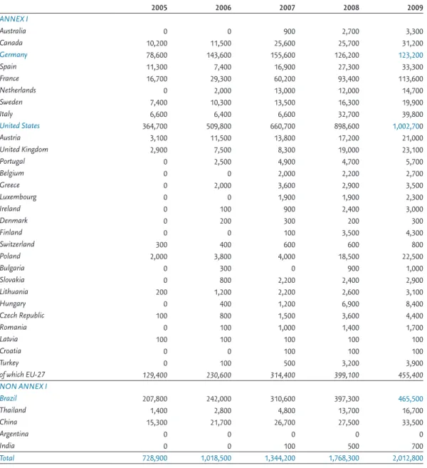
2005 2006 2007 2008 2009 ANNEX I Australia 0 0 900 2,700 3,300 Canada 10,200 11,500 25,600 25,700 31,200 Germany 78,600 143,600 155,600 126,200 123,200 Spain 11,300 7,400 16,900 27,300 33,300 France 16,700 29,300 60,200 93,400 113,600 Netherlands 0 2,000 13,000 12,000 14,700 Sweden 7,400 10,300 13,500 16,300 19,900 Italy 6,600 6,400 6,600 32,700 39,800 United States 364,700 509,800 660,700 898,600 1,002,700 Austria 3,100 11,500 13,800 17,200 21,000 United Kingdom 2,900 7,500 8,300 19,000 23,100 Portugal 0 2,500 4,900 4,700 5,700 Belgium 0 0 2,000 2,200 2,700 Greece 0 2,000 3,600 2,900 3,500 Luxembourg 0 0 1,900 1,900 2,300 Ireland 0 100 900 2,400 3,000 Denmark 0 200 300 200 300 Finland 0 0 100 3,500 4,300 Switzerland 300 400 600 600 800 Poland 2,000 3,800 4,000 18,500 22,500 Bulgaria 0 300 0 900 1,000 Slovakia 0 800 2,200 2,400 2,900 Lithuania 200 1,200 2,200 2,600 3,100 Hungary 0 400 1,200 6,900 8,400 Czech Republic 100 800 1,500 3,600 4,400 Romania 0 100 1,000 1,400 1,700 Latvia 100 100 100 100 100 Croatia 0 0 100 100 100 Turkey 0 100 500 3,200 3,900 of which EU-27 129,400 230,600 314,400 399,100 455,400 NON ANNEX I Brazil 207,800 242,000 310,600 397,300 465,500 Thailand 1,400 2,800 4,800 13,700 16,700 China 15,300 21,700 26,700 27,500 33,500 Argentina 0 0 0 0 0 India 0 0 100 500 700 Total 728,900 1,018,500 1,344,200 1,768,300 2,012,800
Note: Data for 2009 were extrapolated using total global production data, except for Germany, the USA and Brazil (shown in blue).
heating per household (e.g., much more in Moscow than in Los Angeles or New Delhi).
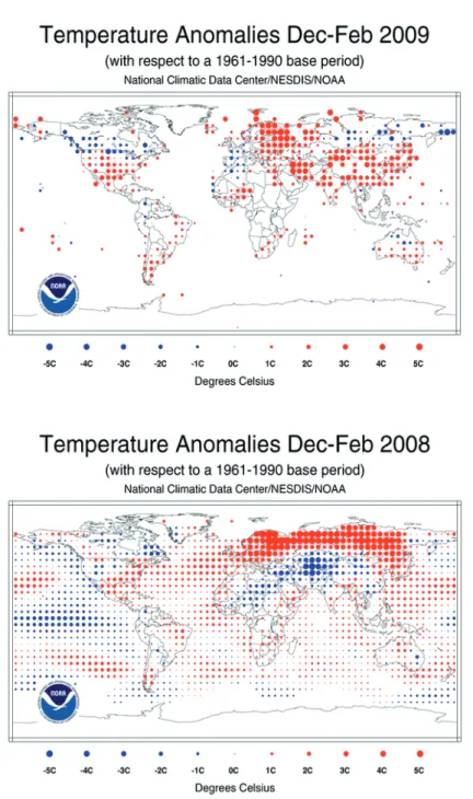
A global analysis by NOAA/NCDC (2008; 2009) characterised the winter months of 2009 as follows:
January-February 2009. Anomalously warm temperatures covered much of the global land area. Warmer-than-average temperatures occurred in most land areas except cooler-than-average conditions across parts of western Alaska, north-western South America, north-central continental USA, south-eastern Canada, northern Australia, north-western Africa, north-western Europe, and central and eastern Russia. In Europe, bitter cold temperatures gripped the northern and eastern region at the beginning of January. September-November 2009.Warmer-than-average
temperatures engulfed much of the planet’s surface, with the exception of cooler-than-average conditions across central Asia, southern South America, and parts of the central contiguous USA.
December 2009. The worldwide land surface temperature tied with 1915 as the 31st warmest December on record. Warmer-than-average conditions were observed across Alaska, eastern Canada, Australia, eastern Russia, southern Europe, southern Asia, and parts of northern Africa and northern South America. Cooler-than-average conditions engulfed much of the contiguous United States, south-western and south central Canada, northern Kazakhstan, Mongolia, northern China, and most of Russia. Other areas with below average conditions include New Zealand, Argentina, and southern Chile. It was abnormally cool across the United Kingdom, and Ireland experienced its coolest December in 28 years.
A similar analysis by NOAA/NCDC (2008) for the winter months of 2008 concluded:
January-February 2008. Cooler-than-average temperatures across the Middle East region, Kazakhstan, Mongolia, Alaska, parts of the western and north-central contiguous USA, northern Africa, and most of China. Warmer-than-average temperatures across Europe, western and central
Russia, central and western Australia, and the southern Plains to the eastern Great Lakes of the contiguous USA. September-November 2008. Warmer-than-average
temperatures across Asia, the western and north-central contiguous USA, eastern Brazil, most of Australia, Europe, and the southern countries in South America. Cooler-than-average conditions occurred across eastern Europe, southern Alaska, south-central and south-eastern continental USA, and parts of Mexico.
December 2008. Warmer-than-average temperatures in Iceland, Fenno-Scandinavia, western and eastern Russia, western Alaska, the eastern contiguous USA, western and south-eastern Africa, eastern Europe, western Australia, and most of Mexico, South America, and southern and south-eastern Asia. Cooler-than-average conditions were present across Canada, the central and north-western continental USA, central Russia, north-western Europe, western and southern Australia, and parts of the Middle East Region.
The difference in demand for space heating in the Northern Hemisphere winter months in 2008 and 2009 is shown visually in Figure A3.1, which presents NOAA maps showing the spatial distribution of temperature anomalies for the winter periods (December-February) for these two years.
Heating-Degree Days (HDD-15) for selected cities in 2009 compared with 2008
Country City HDD 2008 HDD 2009 Difference
China Beiijing 2316 2460 6%
Shanghai 1176 1118 -5%
India New Delhi 219 154 -30%
Mumbai 0 0 Japan Tokyo 1031 940 -9% Osaka 1178 1114 -5% Russia Moscow 3414 3837 12% Italy Rome 973 1017 5% Germany Berlin 2174 2394 10% Düsseldorf 1994 2033 2% Netherlands Amsterdam 1992 2028 2%
United Kingdom London 1750 1733 -1%
United States New York 1772 1880 6%
Washington, DC 1512 1682 11%
Atlanta 1070 1065 0%
Los Angeles 327 330 1%
Source: http://www.degreedays.net using 15o C as threshold temperature.
No growth in total CO2 emissions in 2009
References
Barros, S. (2010), Brazil Sugar Annual 2010. GAIN report no. BR-10002. USDA.
BMU (2010), Development of Renewable Energy Sources in Germany 2009. 18 March 2010. Federal Ministry for the Environment, Nature Conservation and Nuclear Safety (BMU) Division KI II 1.
BP (2010), BP Statistical Review of World Energy 2009.
China Weekly News (2010), 2009 Chinese Cement Production Amounted to 1.63 Billion Tons, a Rise of 17.91%.(Report). 23 March 2010. CRF (2010). Common Reporting Format files of Annex I countries
submitted to UNFCCC Secretariat.
Den Elzen, M.G.J., M. Roelfsema and S. Slingerland (2009), Too hot to handle? The emission surplus in the Copenhagen negotiations. Report no. 500114016. PBL, Bilthoven.
EBB (European Biodiesel Board) (2010), Statistics. The EU biodiesel industry.
Eickhout, B., G.J. van den Born, J. Notenboom, M. van Oorschot, J.P.M. Ros, D.P. van Vuuren and H.J. Westhoek, (2008), Local and global consequences of the EU renewable directive for biofuels. Testing the sustainability criteria. Report no. 500143001. PBL, Bilthoven. Edwards, R., J-F. Larivé, V. Mahieu and P. Rouveirolles (2008),
Well-to-Wheels analysis of future automotive fuels and powertrains in the European context. TANK-to-WHEELS Report; Version 3, October 2008. JRC/CONCAWE/EUCAR, Ispra.
EIA (2010), U.S. Carbon Dioxide Emissions in 2009: A Retrospective Review. Energy Information Administration, U.S. Department of Energy, 5 May 2010.
Comparison of global temperature anomalies for the winter periods of 2008 and 2009. Source: NOAA/NCDC,
2008; 2009).
Figure A3.1 Comparison of global temperature anomalies in the winters of 2008 and 2009
EIA (2010b), May 2010 Monthly Energy Review. Table 2.5, Release Date: May 27, 2010.
EPIA (2010), Global Market Outlook for Photovoltaics until 2014. May 2010 update. European Photovoltaic Industry Association, Brussels. GCP (Global Carbon Project) (2010), Internet http://www.
globalcarbonproject.org/.
Gregg, J.S., R.J. Andres and G. Marland (2008), China: Emissions pattern of the world leader in CO2 emissions from fossil fuel
consumption and cement production. Geophys. Res. Lett., 35, L08806,
doi:10.1029/2007GL032887.
GGFR (Global Gas Flaring Reduction Partnership) (2010), Gas flaring estimates for 2008.
GRFR (2010), Global ethanol production to reach 85.9 billion litres in 2010, 21 March 2010. Global Renewable Fuels Alliance.
GWEC (2010), Global wind 2009 report. Global Wind Energy Council. Hooijer, A., M. Silvius, H. Wösten and S. Page (2006), PEAT-CO2,
Assessment of CO2 emissions from drained peatlands in SE Asia. Delft
Hydraulics. Report Q3943.
IEA (2009), CO2 from fuel combustion. 2009 Edition. International Energy
Agency, Paris.
IMF (2010), World Economic Outlook Database, International Monetary Fund, April 2010.
IPCC (1996), Revised 1996 IPCC Guidelines for National Greenhouse Gas Emission Inventories. Three volumes: Reference manual, Reporting Guidelines and Workbook. IPCC/OECD/IEA. IPCC WG1 Technical Support Unit, Hadley Centre, Meteorological Office, Bracknell, UK.
IPCC (2006), 2006 IPCC Guidelines for National Greenhouse Gas Inventories. Prepared by the National Greenhouse Gas Inventories Programme (NGGIP), Eggleston H.S., L. Buendia, K. Miwa, T. Ngara and K. Tanabe (eds), IGES, Japan.
JRC/PBL (European Commission, Joint Research Centre (JRC)/Netherlands Environmental Assessment Agency (PBL) (2009), Emission Database
for Global Atmospheric Research (EDGAR), release version 4.0. Internet:
http://edgar.jrc.ec.europa.eu
JRC/PBL (European Commission, Joint Research Centre (JRC)/Netherlands Environmental Assessment Agency (PBL) (2010), Emission Database
for Global Atmospheric Research (EDGAR), release version 4.1. In prep.
Internet: http://edgar.jrc.ec.europa.eu
Marland, G., A. Brenkert and J.G.J. Olivier (1999), CO2 from fossil fuel
burning: a comparison of ORNL and EDGAR estimates of national emissions. Environmental Science & Policy, 2, 265-274.
Olivier, J.G.J. and J.A.H.W. Peters (2002), Uncertainties in global, regional and national emission inventories. In: Van Ham, J., A.P.M. Baede, R. Guicherit and J.F.G.M. Williams-Jacobse (eds.):‘Non-CO2 greenhouse gases: scientific understanding, control options and policy aspects. Proceedings of the Third International Symposium, Maastricht, Netherlands, 21-23 January 2002’, pp. 525-540. Millpress Science Publishers, Rotterdam. ISBN 90-77017-70-4.
NOAA/NCDC (2007, 2008, 2009), Climate of 2007/2008/2009. February in Historical Perspective. Including Boreal Winter. National Climatic Data Center, March 2007/2008/2009. NOAA/NCDC (2007, 2008, 2009), Climate of 2007/2008/2009. February in Historical Perspective. Including Boreal Winter. National Climatic Data Center, March 2007/2008/2009. REN21 (2009), Renewables Global Status Report. 2009 update. REN21
Secretariat, Paris.
Renewable Energy Magazine (2010), Global biodiesel market almost doubles every year between 2001 and 2009, 6/4/2010.
Reuters (2009a), European recession slashed 2009 carbon emissions. 18 May 2010.
Reuters (2009b), Global CO2 emissions about 2.6 pct down in 2009-IEA. 21
September 2009.
Reuters (2010), U.N. forecasts less than 1 billion Kyoto offsets by 2012. 6 May 2010. Internet:
Ros, J.P.M., K.P. Overmars, E. Stehfest, A.G. Prins, J. Notenboom and M. van Oorschot (2010), Identifying the indirect effects of bio-energy production. Report no. 500143003. PBL, Bilthoven.
Systèmes solaires (2007), Biofuels barometer 2007 - EurObserv’ER, Systèmes solaires, Le journal des énergies renouvelables n° 179, s. 63-75, 5/2007.
Systèmes solaires (2008), Biofuels barometer 2008 - EurObserv’ER, Systèmes solaires, Le journal des énergies renouvelables n° 185, p. 49-66, 6/2008.
Systèmes solaires (2009), Biofuels barometer 2009 - EurObserv’ER, Systèmes solaires, Le journal des énergies renouvelables n° 192, p. 54-77, 7/2009.
UNEP/NFI (2009), Global Trends in Sustainable Energy Investment 2009. Analysis of Trends and Issues in the Financing of Renewable Energy and Energy Efficiency. ISBN: 978 92 807 3038 1. UNEP DTIE, Energy Branch, Energy Finance Unit, Paris.
USGS (U.S. Geological Survey), 2010. Cement Statistics and Information. Van Dijk, P.M., C. Kuenzer, J. Zhang, K.H.A.A. Wolf and J. Wang (2009),
Fossil Fuel Deposit Fires. Occurrence Inventory, design and assessment of Instrumental Options. WAB report 500102021. PBL, Bilthoven.
Van der Werf, G.R., J.T. Randerson, L. Giglio, G.J. Collatz, P.S. Kasibhatla and A.F. Arellano, Jr (2006), Interannual variability in global biomass burning emissions from 1997 to 2004. Atmos. Chem. Phys., 6, 3423-3441. Van der Werf, G.R. , J. Dempewolf, S.N. Trigg, J.T. Randerson, P.S.
Kasibhatla, L. Giglio, D. Murdiyarso, W. Peters, D.C. Morton, G.J. Collatz, A.J. Dolman and R.S. DeFries (2008), Climate regulation of fire emissions and deforestation in equatorial Asia, PNAS, 150, 20350–20355. Van der Werf, G.R., J.T. Randerson, L. Giglio, G.J. Collatz, M. Mu, P.S.
Kasibhatla, D.C. Morton, R.S. DeFries, Y. Yin and T.T. van Leeuwen (2010), Global fire emissions and the contribution of deforestation, savanna, forest, agricultural, and peat fires (1997-2009). Internet:
http://www.falw.vu/~gwerf/GFED/
WBCSC (2009), Cement Industry Energy and CO2 Performance: ‘Getting the Numbers Right’. World Business Council for Sustainable Development.
WSA (2010), Crude steel production statistics. World Steel Association.
Colophon Responsibility
Netherlands Environmental Assessment Agency
Authors
J.G.J. Olivier, J.A.H.W. Peters
Graphics
M. Abels, J.A.H.W. Peters
Editing
H.J. West
Design and layout
Uitgeverij RIVM
Corresponding Author