Onzekerheids- en gevoeligheidsanalyse van GeoPEARL

Hele tekst

(1)Uncertainty and sensitivity analysis of GeoPEARL. F. van den Berg D.J. Brus S.L.G.E. Burgers G.B.M. Heuvelink J.G. Kroes J. Stolte A. Tiktak F. de Vries. Alterra-report 1330, ISSN 1566-7197 PBL-rapport 500123001. Uitloop 0 lijn. 20 mm 15 mm 10 mm 5 mm. 0 15 mm. 0 84 mm. 0 195 mm.

(2) Uncertainty and sensitivity analysis of GeoPEARL.

(3) 2. Alterra-report 1330.

(4) Uncertainty and sensitivity analysis of GeoPEARL. F. van den Berg D.J. Brus S. L.G.E. Burgers G.B.M. Heuvelink J.G. Kroes J. Stolte A. Tiktak F. de Vries. Alterra-report 1330 Alterra, Wageningen, 2008.

(5) ABSTRACT Berg, F. van den, D.J. Brus, S.L.G.E. Burgers, G.B.M. Heuvelink, J.G. Kroes, J. Stolte, A. Tiktak & F. de Vries. 2008. Uncertainty and sensitivity analysis of GeoPEARL. Wageningen, Alterra, Alterra-report 1330, PBL-rapport 500123001. 114 blz.; 24 figs.; 22 tables.; 57 refs. In the environmental assessments by the Netherlands Environmental Assessment Agency (PBL), the GeoPEARL model is used to calculate the leaching of pesticides to the groundwater at the national scale. In this study, the propagation of errors resulting from the use of a simplified spatial schematisation as well as that of uncertainties in the GeoPEARL input to the predicted leaching concentrations were investigated. Computations using GeoPEARL with the standard schematisation were compared with those obtained with a schematisation at a higher spatial resolution. For all three pesticides considered the nationwide spatial frequency distribution of the median annual leaching concentration (PEC50) and the spatial 90th percentile of the PEC50 (SP90) were hardly affected by spatial aggregation of soil type within larger spatial units. For the assessment of the propagation of uncertainties in the input, only soil properties and the most important pesticide properties, i.e. half-life in soil (DT50) and the coefficient for the sorption on organic matter (Kom) were considered. First, the uncertainties in the soil data and the pesticide were quantified. Next, a regular grid sample of points covering the whole of the agricultural area in the Netherlands was randomly selected. At the grid nodes, realisations from the probability distributions of uncertain inputs were generated and used as input to a Monte Carlo uncertainty propagation analysis. Uncertainties in DT50 and to a lesser extent Kom contributed most to the uncertainty in PEC50 and SP90. The uncertainty about the PEC50 at point locations is greater than that about the SP90. When taking the uncertainties into account, the SP90 of the leaching concentration shifted towards greater values. Recommendations are made for further improvement of the model predictions, in particular by reducing the uncertainty in DT50. Keywords: error propagation, distribution function, groundwater, half-life, leaching concentrations, pesticide, soil properties, sorption coefficient, spatial aggregate ISSN 1566-7197. This report is available in digital format at www.alterra.wur.nl. A printed version of the report, like all other Alterra publications, is available from Cereales Publishers in Wageningen (tel: +31 (0) 317 466666). For information about, conditions, prices and the quickest way of ordering see www.boomblad.nl/rapportenservice. © 2008 Alterra P.O. Box 47; 6700 AA Wageningen; The Netherlands Phone: + 31 317 484700; fax: +31 317 419000; e-mail: info.alterra@wur.nl No part of this publication may be reproduced or published in any form or by any means, or stored in a database or retrieval system without the written permission of Alterra. Alterra assumes no liability for any losses resulting from the use of the research results or recommendations in this report.. 4. Alterra-report 1330 [Alterra-report 13303/June/2008].

(6) Contents Preface. 7. Summary. 9. 1. 2. 3. 4. Introduction 1.1 Uncertainty about pesticide leaching 1.2 Model inputs and outputs 1.3 Objectives of research 1.3.1 Analysis of the error resulting from the use of a simplified soil physical-chemical map 1.3.2 Uncertainty in leaching concentrations at the field scale and at the scale of the total agricultural area in the Netherlands 1.4 Outline of report Analysis of errors in leaching concentrations resulting from the use of the simplified soil physical-chemical map 2.1 Introduction 2.2 Geochemical-geophysical-hydrological map used by STONE 2.3 Detailed soil physical-chemical map 2.4 Procedure of model calculations 2.5 Results of GeoPEARL calculations 2.6 Conclusions Uncertainty and sensitivity analysis of GeoPEARL 3.1 Identification and stochastic simulation of uncertain soil properties 3.1.1 Probability distributions for uncertain soil properties 3.1.2 Parameter values for probability distributions of uncertain soil properties 3.1.3 Stochastic simulation of uncertain soil properties 3.2 Identification and stochastic simulation of uncertain pesticide properties 3.3 Required data on soil properties and locations 3.4 Sensitivity analysis 3.5 Design of the input-matrix in a regression-free sensitivity analysis 3.6 Checks on GeoPEARL input 3.7 GeoPEARL simulations. 11 11 12 13 13 15 15 17 17 17 19 21 22 23 25 26 27 34 38 40 42 44 46 48 49. Results of the uncertainty and sensitivity analysis of GeoPEARL 51 4.1 PEC50 at point locations 51 4.1.1 PEC50 at all locations 51 4.1.2 Uncertainty analysis at the six locations 52 4.1.3 Sensitivity analysis for the six locations : regression-free 55 4.1.4 Sensitivity analysis for the six locations by spline regression 61 4.2 Results for 90th percentile of spatial cumulative frequency distribution of PEC50 63 4.2.1 Uncertainty analysis of the SP90 63 4.2.2 Sensitivity analysis of the SP90 67.

(7) 5. 6. Discussion 5.1 Quantification of the error resulting from the use of simplified physical-chemical soil map 5.2 Effect of uncertainty of pesticide properties and soil characteristics on the median annual average leaching concentrations at locations 5.3 Effect of uncertainty of pesticide properties and soil characteristics on the spatial 90th percentile of the leaching concentrations 5.4 Assessment of the contribution of individual uncertain input parameters to the total uncertainty in PEC50 and SP90 5.5 Effect of other uncertainties on the spatial 90th percentile of the leaching concentration 5.6 Proposal of a strategy to reduce the uncertainty of the current GeoPEARL simulations Conclusions and recommendations 6.1 Conclusions 6.2 Recommendations. 70 71 72 73 74. 83. 1 Classification tree Staring series building blocks 2 Example SOL file 3 Parameters of the fitted lognormal distributions for organic matter content. 6. 69. 77 77 78. Literature. Appendices. 69. 89 99 101. Alterra-report 1330.

(8) Preface. Quality assurance of environmental models used in assessments by the Netherlands Environmental Assessment Agency (PBL) is important. As a result of an inventory of the quality of the models used by Wageningen UR for these assessments, the research programme ‘KwaliteitsSlag’ was set up to improve the quality of these models. This programme started in 2006 and was financed by PBL and Wageningen UR. One of the projects in this research programme dealt with the uncertainty in the calculation of the leaching of pesticides to the groundwater at the national scale as calculated with the GeoPEARL model. In this report the results of a study on the uncertainty in leaching concentrations over time at a specific location and in the spatial leaching concentration over the entire agricultural area are presented. Further, the effects of a simplification in the chemical-physical soil map on the spatial leaching concentrations at the national scale is assessed.. Alterra-report 1330. 7.

(9)

(10) Summary. In the environmental assessments by the Netherlands Environmental Assessment Agency (PBL), the GeoPEARL model is used to calculate the leaching of pesticides to the groundwater at the national scale. The target quantity to report the risk of leaching at a specific location is the 50th percentile over time of the predicted annual average concentration in soil (PEC50). The concentration is taken at 1 m soil depth, which is considered to be representative for the concentration in the upper groundwater. In the new Dutch decision tree for leaching of pesticides to groundwater within the registration procedure of pesticides, the 90th percentile of the spatial frequency distribution (spatial P90 or SP90) of the PEC50 is taken in its area of use. In this report the effect of a simplification in the Dutch physical-chemical soil map on the spatial leaching concentrations was assessed. First, a detailed physicalchemical soil map was prepared based on the 1:50 000 soil map of the Netherlands. Input data on soil properties for GeoPEARL were derived from the simplified soil map as used in the current PBL assessments and from the detailed physical-chemical soil map. The 90th percentile leaching concentrations at a depth of 1 m calculated for both physical-chemical soil maps were compared. The results show that the spatial P90s for the Netherlands as a whole calculated with both soil maps do not differ much. However, the spatial P90s for smaller areas (regions) may differ substantially. In this report also the propagation of uncertainty about important soil and pesticide properties to the PEC50 and SP90 was studied. The soil properties taken into consideration were clay content, silt content, sand content, organic matter content, hydraulic characteristics, and thickness of the soil horizons. The probability distributions for texture, horizon thickness and organic matter were derived from data in the Dutch Soil Information System. Data on the water retention and hydraulic conductivity characteristics of soils were taken from the Staring Series, which is a database containing multiple measurements of 36 different building blocks (for top- and subsoil). The set of curves of a building block was treated as a random sample from all curves that populate the building block. The uncertain pesticide properties considered were the coefficient for the sorption on organic matter and the half-life of transformation in soil. The uncertainty in the pesticide properties was characterised by their variability between soils, which was derived from literature studies. Stochastic simulations at six point locations showed that uncertainty about PEC50 at point locations is large, also at the 0.1 μg/L level. The spatial pattern of the median leaching concentration over time (PEC50) in the Monte Carlo simulations corresponded well with the spatial pattern predicted in an ordinary deterministic GeoPEARL run. Both in the stochastic simulation and in the deterministic simulation, there is a strong correlation between PEC50 and organic matter. For the. Alterra-report 1330. 9.

(11) PEC50, the pesticide transformation half-life (DT50) is the main source of uncertainty. The contributions of the sorption coefficient (Kom) and organic matter to the total uncertainty were smaller, but meaningful. The contribution of uncertainty in texture and soil physical properties to the total uncertainty is generally small. The uncertainty about the spatial P90 (SP90) – which is the regulatory endpoint in Dutch pesticide registration – is smaller than the uncertainty about PEC50 at point locations. The width of the interquartile range is computed to be 15% of the median spatial P90 for pesticides A and B and approximately 40% in the case of pesticide D. For the 90th percentile leaching concentration in space, the most important source of uncertainty on the model output was DT50 and to a lesser degree Kom. Moreover, the estimated 90th percentile concentrations are substantially larger when uncertainty of pesticide and soil properties is considered. The important implication for regulation is that the SP90 is systematically underestimated when uncertainty is ignored. However, when uncertainty is included in the analysis, it may be sensible to use a less extreme percentile for regulatory evaluation, such as the 80th percentile. In this study several assumptions were made. Firstly, it was assumed that the Dutch 1:50 000 soil map was free of errors. This results in an underestimation of the contribution of the uncertainty about the basic soil properties to the total uncertainty about the pesticide leaching. Secondly, lateral and vertical correlations (between soil layers) in the uncertainty of the soil and pesticide properties were ignored. Taking these correlations into account will likely result in an increase in the uncertainty in the SP90. Before this can be done, statistical models and software that describe this correlation need to be improved. The degradation half-life is by far the most important source of uncertainty of both the PEC50 at individual locations and the spatial P90. Strategies to reduce the overall uncertainty should therefore first be directed towards obtaining better estimates of the degradation half-life and its dependence on soil type. As GeoPEARL requires a lot of computation time, it is recommended to check whether part of the analyses could be done with a simpler model. A prerequisite is that the simple model captures the most important processes and shows the same behaviour as the complex model. The soil organic matter map can be improved by including the soil data in the TAGA-archives. This will result in a more accurate soil organic matter map and will yield improved spatial patterns of PEC50. For an overall assessment of the effect of uncertainties in the model input on the target output, uncertainty in other input data, such as the bottom boundary condition, the dispersion length, land use data and drainage data should be investigated. By ranking the effects of all sources of uncertainty, the weakest parts of the GeoPEARL model chain can be identified and a prioritization can be presented for further improvement of the model.. 10. Alterra-report 1330.

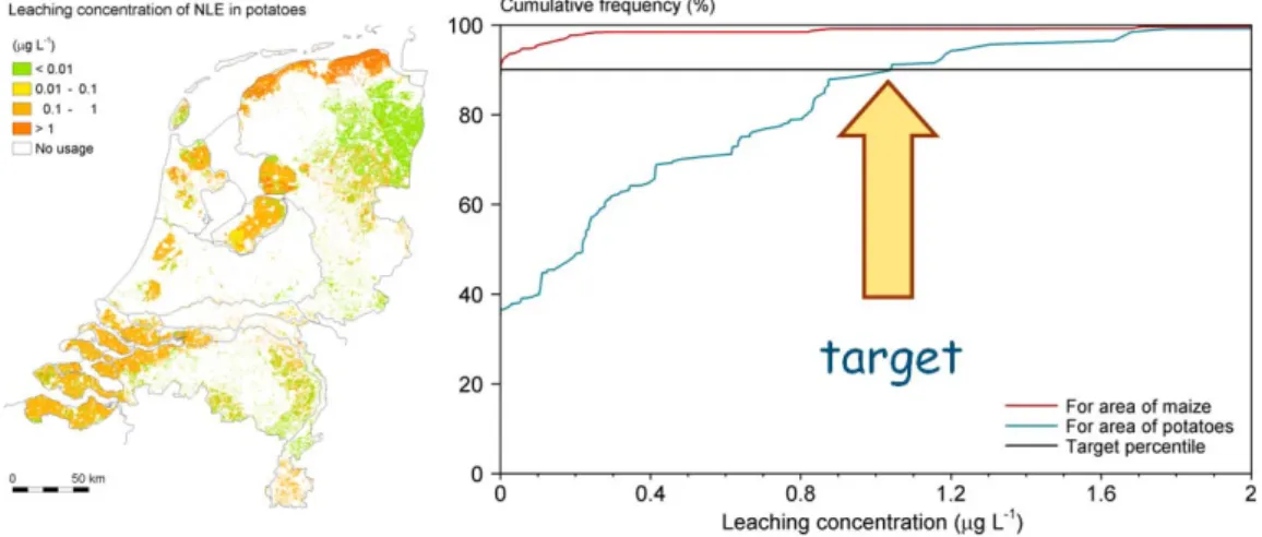
(12) 1. Introduction. 1.1. Uncertainty about pesticide leaching. In the Netherlands a policy plan on sustainable crop protection has been adopted to ensure that environmental risks due to the use of crop protection products (pesticides) are minimised (LNV, 2004). The Netherlands Environmental Assessment Agency (PBL) is responsible for evaluating the progress made in achieving the objectives of this plan. Pesticide leaching to the groundwater is one of the aspects considered, because groundwater is a major source of drinking water in the Netherlands. The PBL uses a metamodel of the GeoPEARL model to assess the leaching of pesticides to the groundwater (Van der Linden et al., 2006). GeoPEARL is a spatially distributed pesticide leaching model (Tiktak et al., 2002; 2003), which combines a one-dimensional, process-based leaching model to spatial data available in Geographical Information Systems. GeoPEARL also plays a central role in Dutch pesticide registration procedures (Van der Linden et al., 2004). In contrast to earlier procedures (Van der Linden and Boesten, 1989), pesticide leaching is evaluated in the entire intended use area of the product. A pesticide can only be registered if the concentration of the pesticide is below 0.1 μg/L for more than 90% of the intended use area of the product. This regulatory endpoint can be directly inferred from the cumulative frequency distribution of the predicted leaching concentration in the intended use area (Figure 1.1).. Figure 1.1. Percentiles of the leaching concentration in the intended use area can be inferred from the cumulative frequency distribution of a leaching map. Example with pesticide “NLE” in potatoes (as in Tiktak et al., 2003).. Until now, uncertainty is not explicitly addressed in the risk assessment. However, understanding the consequences of uncertainty is needed to improve risk assessment as a decision-support tool (Brown and Heuvelink, 2005; Refsgaard and Henriksen, 2004). The different sources of uncertainty in pesticide fate modelling have been. Alterra-report 1330. 11.

(13) described by Dubus et al. (2003). Uncertainty is first present in the primary data (physical, chemical and environmental conditions). There is also uncertainty in the estimation of model input parameters from these primary data. This includes for example the estimation of pesticide half-life (DT50) from laboratory data, even though harmonization of the boundary conditions and settings can limit this source of uncertainty (FOCUS, 2006). Uncertainty in environmental assessments also arises from the use of pedotransfer functions (Tiktak et al., 1999; Dubus et al., 2003) or the use of spatial interpolation of spatially referenced parameters (Brus and Jansen, 2004; Brown and Heuvelink, 2005). Model structure, the numerical solution of the model and the spatial schematisation provide additional sources of uncertainty (Addiscott et al., 1995). Jury and Gruber (1989) and Van der Zee and Boesten (1991) have studied the effect of spatial variability on the average leached fractions of the applied dosage of pesticides from fields by stochastic simulation, and they suggested that spatial variability can significantly increase the pesticide leaching. Leterme et al. (2007) studied the effect of spatial variability on pesticide leaching on a regional scale using a similar method and their findings also indicate an increase in the fractions of the dosage of pesticide leached. Stochastic simulations are likely to generate extreme events that are not captured within an ‘average’ deterministic simulation.. 1.2. Model inputs and outputs. This report presents an uncertainty and sensitivity analysis of the GeoPEARL model. The analysis only studies the effect of input uncertainty. GeoPEARL contains a large number of model inputs (Figure 1.2), many of which are spatially distributed. An uncertainty analysis with all these model inputs would require too much computation time, because a single GeoPEARL run requires approximately 24 hours on a single computer. The analysis therefore focuses on the uncertainty of the pesticide half-life (DT50), the coefficient for sorption on organic matter (Kom), soil organic matter content, soil texture, thickness of soil horizons, Staring series building blocks and the soil physical properties of the Staring series building blocks. The choice of these (sets of) input parameters follows the conclusions of Tiktak et al. (1994) and Boesten (1991) in previous sensitivity analyses performed on the point-scale models PESTRAS and PESTLA, respectively. These two models are predecessors of the PEARL model. They found the Freundlich exponent, Kom, and DT50 to be the most sensitive pesticide parameters. Organic matter content was found to be the most important soil parameter. Other sensitive parameters were the soil physical parameters, in particular the n-parameter in the Mualem-van Genuchten equation of water retention, and the saturated conductivity parameter Ksat. The Freundlich exponent was not included in the analysis presented in this report. Uncertainty in the Freundlich coefficient is considered to be less important than that in the half-life and the sorption coefficient, because the coefficient of variation of the Freundlich exponent is much smaller than that of half-life and sorption coefficient.. 12. Alterra-report 1330.

(14) Substance Substance properties, such as the half-live and the partitioning coefficient. Management Application date Application type Application dosage. Assessment Substance ID Plot ID Management ID Start date End date Output control. Meteo district Rainfall Temperature ETref. Soil profile Soil layer ID. Plot Meteo district ID Land-use type ID Soil profile ID Groundwater depth group ID Seepage flux and amplitude Drainage characteristics Irrigation switch. Spatially distributed variables. Soil layer Soil physical unit ID Layer thickness Texture Organic matter pH. Soil physical unit Parameters of the Mualemvan Genuchten functions Dispersion length. Groundwater depth group Initial groundwater level. Land-use Emergence date Harvest date Development stage ID Critical pressure heads for drought stress and irrigation. Development stage LAI Crop factor Rooting depth. Figure 1.2 Structure of the GeoPEARL database. Fields in yellow refer to spatially distributed inputs, fields in green are assumed spatially constant in deterministic studies.. The uncertainty analysis focused on the following model outputs: - The temporal median of the annual average leaching concentration (PEC50) at 1 m depth at point locations within the intended use area. Following FOCUS (2000), the median annual average leaching concentration is derived from a weather time-series of 20 years. So, to calculate the PEC50 at a location, the following procedure is followed: (i) at the location of interest, the point scale model PEARL is run for 20 years with real weather data, (ii) the annual average leaching concentrations are calculated for these 20 years, (iii) PEC50 is computed by taking the median of these 20 averages; - The 90th percentile of the spatial distribution of PEC50 in the intended use area (SP90). In our analysis, it is assumed that the intended use area is the entire agricultural area within the Netherlands.. 1.3. Objectives of research. 1.3.1. Analysis of the error resulting from the use of a simplified soil physical-chemical map. Although more detailed spatial information of the soil input is available for the Netherlands, in a standard assessment of the target concentration, computations are done for 6 405 map units, referred to as ‘STONE plots’ (Kroon et al., 2001). These. Alterra-report 1330. 13.

(15) plots are characterised by unique combinations of subsoils (‘hydrotypes’), drainage characteristics, seepage fluxes, groundwater depth classes, land use type, climate district, soil physical type and soil profiles (Figure 1.3). This saves considerable computing time because GeoPEARL needs only be run 6 405 times, since all locations within a STONE-plot have the same input values. However, ignoring spatial variation within plots may lead to bias (Heuvelink and Pebesma, 1999), particularly for non-linear models such as GeoPEARL (Leterme et al., 2007). The bias may be quantified by comparing the standard GeoPEARL results with the results obtained with a more detailed map of model inputs. Because of time constraints, the analysis of the effect of accounting for spatial variation of input variables within the 6 405 STONE-plots was limited to soil input characteristics. More detailed maps of the hydrological and climatic input variables were not used. Instead, these input variables were derived from the STONE map with 6 405 map units (plots). The research presented in the first part of this report (Chapter 2) therefore focuses on the quantification of the error resulting from the use of a spatial schematisation, consisting of 6 405 unique combinations.. Figure 1.3 Procedure for creating the spatial schematisation for GeoPEARL. This procedure was originally developed for the Dutch Model for Emission of Nutrients, STONE (Kroon et al., 2001). 14. Alterra-report 1330.

(16) 1.3.2 Uncertainty in leaching concentrations at the field scale and at the scale of the total agricultural area in the Netherlands The main objective of this study was to analyse the uncertainty in the leaching concentration calculated with the GeoPEARL model at specific locations as well as at the scale of the entire agricultural area within the Netherlands. As a complete analysis for all components in the GeoPEARL model, e.g the lower boundary flux, drainage schematisation, would be very time consuming, the uncertainty analysis focussed on the soil schematisation and the two most important pesticide properties, i.e. the coefficient for the sorption on organic matter and the half-life in soil. The research presented in chapters 3 and 4 therefore focuses on: 1. Quantification of the uncertainty about the median annual average leaching concentration at point locations (PEC50) and about the associated spatial 90thpercentile for the entire Dutch agricultural area (spatial P90, abbreviated here to SP90), as caused by uncertainty of pesticide properties and soil characteristics; 2. Assessment of the contribution of individual uncertain input parameters to the total uncertainty in PEC50 and SP90 (i.e. stochastic sensitivity analysis). Other important issues addressed in this report are 1) whether ignoring uncertainty in soil characteristics and pesticide properties leads to a systematic error (bias) in the model predictions and 2) what strategy should be followed to reduce the uncertainty of the current GeoPEARL simulations.. 1.4. Outline of report. In Chapter 2 the effect of accounting for spatial variation in soil input variables within STONE plots is quantified. This chapter first presents a more detailed map with soil input variables. Using an overlay of the soil map 1:50 000 and the map with the STONE plots, all relevant soil profiles within each STONE plot are characterised. Using the more detailed soil map, the SP90 (i.e., the 90th percentile of the spatial cumulative frequency distribution of the median annual leaching concentration at a depth of 1 m) is assessed for the whole agricultural area. The results of these calculations and the results of the standard schematisation for four different pesticides are also presented. Chapters 3 and 4 present the uncertainty and stochastic sensitivity analysis. Chapter 3 describes the definition, identification and stochastic simulation of soil and pesticide properties. Statistical and technical procedures of the Monte Carlo uncertainty and sensitivity analysis are also presented. The results of the computations are described and interpreted in Chapter 4. Chapter 4 starts with a discussion of results at point locations. The output variable presented is the median average annual leaching concentration (see Section 1.2). Then, the results of the regulatory endpoint (the spatial 90th percentile of the leaching concentration in the entire agricultural area) are discussed.. Alterra-report 1330. 15.

(17) In Chapter 5 the results obtained in the entire study are discussed and compared with results from other studies. Finally, in Chapter 6 recommendations are given for further research and on the improvement of the schematisation as well as the model.. 16. Alterra-report 1330.

(18) 2. Analysis of errors in leaching concentrations resulting from the use of the simplified soil physical-chemical map. 2.1. Introduction. The most important output variable of GeoPEARL is the 90th percentile of the spatial cumulative frequency distribution of PEC50. To obtain an accurate estimate of this percentile, GeoPEARL is run for a large number of unique combinations of soil type, weather district and groundwater depth group (Tiktak et al., 2002; 2003). The current GeoPEARL version uses the so-called STONE schematisation, which was developed for national predictions of nutrient emissions to surface waters and groundwater (Kroon et al., 2001). In this schematisation, the unique combinations are aggregated to 6 405 larger spatial units, using relation diagrams (see also Tiktak et al., 2003). Within each unit, the dominant soil profile is assumed to be representative for the whole unit. The effect of this assumption on the nationwide spatial frequency distribution of predicted PEC50 is analysed by comparing the output of GeoPEARL obtained with the STONE-plot soil input with the output obtained with soil input that is derived from the soil physical-chemical map of De Vries (1999). In Section 2.2 a description is given of the procedure to create the original map with STONE-plots containing information on geochemical, geophysical and hydrological properties, and the information that was added in order to complete the ‘soil’ information required by GeoPEARL. In Section 2.3, the procedure is described to derive a detailed soil physical-chemical map. The output was analysed in detail on the basis of: - the regulatory endpoint for the GeoPEARL model, which is the 90th percentile of the spatial cumulative frequency distribution of the PEC50; - spatial patterns of PEC50. When creating a new map with model inputs, the lower boundary condition of SWAP will be affected. The consequence is that new calculations with NAGROM should preferably be carried out (De Lange, 1996). This step has not been carried out in this study – implying that the current study is limited to the effect of variation of soil input variables within STONE plots only.. 2.2. Geochemical-geophysical-hydrological map used by STONE. In this section a description is given of the procedure followed to obtain the geochemical-geophysical-hydrological map as used by the model STONE. The final map is obtained by overlaying three elementary maps: 1) a geophysical-chemical map of the upper layer, referred to hereafter as the soil physical-chemical map (0-120 cm below surface), 2) a geochemical map of subsurface layers (1.20 - 13 m) and 3) a hydrological map (Kroon et al., 2001).. Alterra-report 1330. 17.

(19) To create the soil physical-chemical map, first the units of the Soil Map of the Netherlands 1: 50 000 are grouped into 21 soil physical units, also referred to as PAWN-units (Figure 2.1, Wösten et al., 1988). With each PAWN-unit a representative soil profile is associated, that is described in terms of a vertical succession of building blocks of the Staring series, including the thickness of the building blocks. The Staring series building blocks are soil horizons, grouped on the basis of soilphysical properties. The 21 soil physical units (PAWN-units) have been subdivided by the Rijksinstituut voor Integraal Zoetwaterbeheer en Afvalwaterbehandeling (RIZA) on the basis of the geochemical properties phosphate sorption capacity, mineralisation capacity and cation exchange capacity (CEC). It should be noted that these parameters are not relevant for pesticide leaching.. Figure 2.1 Map of the 21 soil physical units, also referred to as PAWN-units (Wösten, et al., 1988).. 18. Alterra-report 1330.

(20) Finally, an overlay of the map of the resulting geophysical-chemical units and a land use map with units grassland, maize, other agricultural land use, and nature was made. This results, after aggregation1, in a soil physical-chemical map consisting of 456 map units. For all 456 map units estimates of texture, organic matter content, bulk density, pH, C/N ratio and sesqui-oxide content were added for each layer (Kroon et al., 2001). For this, point-data in the Soil Information System of Alterra, and other information have been used. The subsurface geochemical map is much less detailed, and consists of 30 map units only. The hydrological base-map consists of 900 map units. After overlaying the three elementary maps, the units of the resulting map were grouped into 6405 map units, referred to as STONE-plots, which in fact is a somewhat misleading term because a STONE-plot may consist of multiple map polygons. With this number of map units, the required computing time for one STONE run is one day on a single personal computer, which was considered acceptable. The vertical resolution required by STONE is much larger than that of the representative soil profiles of the 21 PAWN-units (see Appendix 2). Therefore, for each STONE-plot the GeoPEARL layers are allocated on the basis of their depth to one of the Staring series building blocks. All layers within the same building block have the same properties.. 2.3. Detailed soil physical-chemical map. In 1999 a new map of physical and chemical properties of the 0-120 cm soil layer became available (De Vries, 1999). This section describes this new soil physicalchemical map, and how this map was used to obtain the soil data required as input for GeoPEARL. The new soil physical-chemical map is obtained by grouping units of the Soil Map of the Netherlands 1 : 50 000 smaller than 1000 ha with related units (De Vries, 1999). This results in a map of 330 units. Similar to the PAWN-units, each map unit is associated with a representative profile description, that is described in terms of a vertical succession of pedogenetic soil horizons. Note the difference with the representative soil profile descriptions of the PAWN-units, which are described in terms of a vertical succession of Staring series building blocks, i.e. soil physical layers. Each pedogenetic soil horizon is described by median values for thickness of soil horizon, organic mater content, clay fraction, loam fraction sand coarseness (M50), pH-KCl, CaCO3, C/N-ratio and bulk density, as well as a measure of the spatial variation of these properties by means of the 10th- and 90th percentiles. These statistics are derived from point-data in the Soil Information System of Alterra, supplemented by information derived from the descriptions of the sheets of the Soil Map of the Netherlands 1 : 50 000.. 1. Combinations of less than 10 grid cells of 250 m x 250 m have been aggregated.. Alterra-report 1330. 19.

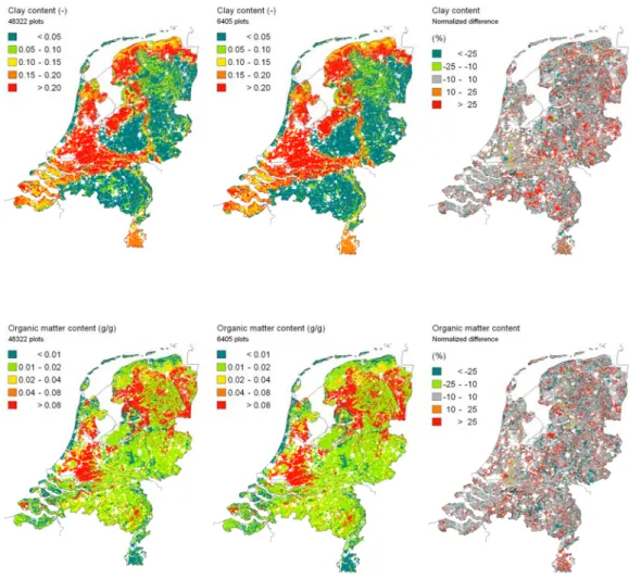
(21) For application of the new soil physical-chemical map in the model GeoPEARL an overlay of this soil physical-chemical map and the map with the 6 405 STONE-plots was made, resulting in 48 423 map units. Most of the STONE-plots contain more than one unit of the detailed soil physical-chemical map. Instead of 6 405, the new GeoPEARL soil file (schematisation.sol file) contains 48 423 different soil profiles. The required information on the basic soil properties such as soil texture, organic mater content and pH-KCl can be directly derived from the 330 representative soil profile descriptions. For this, the median values were used. To determine the Mualem-Van Genuchten parameters, a classification tree was constructed (See Appendix 1). Given soil texture, organic matter content and the geological formation the Staring series building block can be determined, as well as its associated MualemVan Genuchten parameters. It should be noted that in the STONE 2.0 schematisation 456 soil profiles have been defined. This greater number of soil profiles is due to the inclusion of additional soil characteristics, for example CEC and P-binding capacity. These properties are not relevant in the description of pesticide behaviour in soils.. Figure 2.2. Clay content and organic matter content of layer 0 - 120 cm according to the map with STONE-plots (6405 units) and according to the new soil physical-chemical map (48 423 units).. 20. Alterra-report 1330.

(22) Figure 2.2 shows maps of the clay content and organic matter content of the upper 120 cm of the soil profile as derived from the original map with STONE-plots and as derived from the new soil physical-chemical map. At first glance, both for clay content and organic matter content differences between the two maps are small. However, a closer look shows that there are considerable differences, up to 25% (right panel in Figure 2.2).. 2.4. Procedure of model calculations. For the assessment of the effect of the detailed soil physical-chemical map on the predicted spatial 90 percentile leaching concentration, four pesticides were selected. The properties of these pesticides are given in Table 2.1. Pesticides NLA, NLB and NLD are described in FOCUS (2000). Pesticide NLE shows pH-dependent sorption behaviour, and is described in Tiktak et al. (2003). The pesticides were annually applied to the soil surface in spring (26 May). Assessments were made for both the detailed schematisation, and the original STONE schematisation. A beta version of GeoPEARL_3.3.3 was used to calculate the spatial 90th percentile of the leaching concentrations for both schematisations. For the detailed soil schematisation, a schematisation.sol file was prepared, containing the description of the 330 soil profiles. In addition, a new .plo file was constructed containing the soil profile number for all plots in the detailed schematisation. As the leaching concentrations were calculated for the entire agricultural area, ploughing was not considered. Table 2.1 Overview of the most important properties of the pesticides considered in this study. Property1 NLA NLB NLD -1 M (g mol ) 300 300 300 Pv,s (Pa) 0 0.0001 0.0001 90 90 90 Sw (mg L-1) -1 60 10 35 Kom,ac,eq (L kg ) 60 10 35 Kom,ba,eq (L kg-1) Kom,ne (L kg-1) pKa 60 (20 °C) 20 (20 °C) 20 (15 °C) DT50,ref (d) 0 0 0 kd (d-1). NLE 200 0 50 500 25 4.5 50 (20 °C) 0. 1) M is the molar mass, Pv,s is the saturated vapour pressure, Sw is the solubility in water, Kom,ac,eq is the coefficient of equilibrium sorption on organic matter under acidic conditions, Kom,ba,eq is the coefficient of equilibrium sorption on organic matter under basic conditions, Kom,ne is the coefficient of sorption to the non-equilibrium domain, pKa is the negative logarithm of the dissociation constant, DT50,ref is the half-live under reference conditions, and kd is the rate constant for non-equilibrium sorption.. For each pesticide, GeoPEARL was run for the entire agricultural area, so the median leaching concentration at 1 m depth was calculated for all 48324 plots. From these concentrations, GeoPEARL calculated the spatial 90 percentile of the leaching concentration at a depth of 1 m.. Alterra-report 1330. 21.

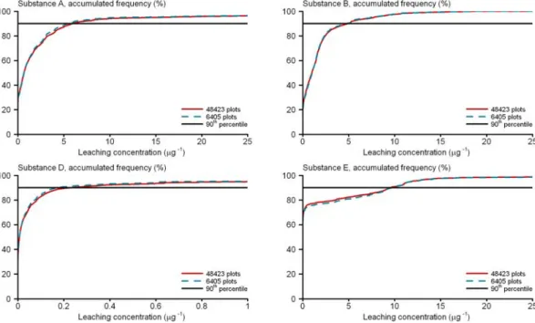
(23) 2.5. Results of GeoPEARL calculations. Comparison of results shows a minor effect of accounting for spatial variation of soil input variables within STONE plots on the nationwide cumulative frequency distribution of the predicted median annual leaching concentration for all pesticides (Figure 2.3).. Figure 2.3. Spatial cumulative frequency distribution of the median annual leaching concentration of four pesticides (see table 3.1 for pesticide properties) calculated with the STONE schematisation (6405 plots) and the detailed soil physical-chemical map (48423 plots).. Also, the spatial 90th percentile leaching concentration was hardly affected by the spatial aggregation of soil type within larger spatial units. Results for PEC50 were also compared on a pixel by pixel basis (grid cell size 250x250 m2). These are shown in Figure 2.4. A first comparison of the spatial patterns does not show large differences. However, when evaluating the normalised differences between the two schematisations, meaningful differences are found (right panel of Figure 2.4). The normalised difference, ND, is calculated as follows: ND = 100. cL , Det − cL , Stone cL , Det. (2.1). In which: cL,Det cL,Stone. = PEC50 (μg/L) calculated using the detailed schematisation = PEC50 (μg/L) calculated using the STONE schematisation. A frequency distribution of the normalised difference shows that 30-40% of the pixels show differences greater than 25% (Table 2.2).. 22. Alterra-report 1330.

(24) Table 2.2 Frequency distribution of the normalised difference between the maps presented in Figure 2.2. ND1 NLA NLB NLD NLE < -25 % 16 15 20 16 -25 - -10 % 2 3 0 1 -10 - +10 % 62 63 60 67 +10 - + 25 % 3 4 0 1 > + 25 % 17 15 20 15 1) calculated according to equation 2.1.. 2.6. Conclusions. The current GeoPEARL schematisation appears to be sufficient for predicting pesticide leaching on the national scale. Local scale predictions are, however, meaningfully affected by spatial aggregation of soil input parameters. This conclusion is in line with earlier conclusions regarding the STONE hydrology (Van Bakel et al., 2002), who advised not to use the STONE schematisation for spatial scales smaller than 25 km2. Acknowledging that there is an increasing need for local-scale model predictions, based on national datasets, Alterra, Deltares and PBL have started the development of the Netherlands Hydrological Instrument (NHI). This new hydrological model will have a larger spatial resolution than the current STONE schematisation. The extended soil schematisation developed in this project can be used as input to the development of this new model.. Alterra-report 1330. 23.

(25) Figure 2.4. Predicted median value of the annual average leaching concentration of four example pesticides at 1-m depth. An annual pesticide dosage of 1 kg ha-1 was used. Left: detailed schematisation, middle: original STONE schematisation, right: normalised difference (%).. 24. Alterra-report 1330.

(26) 3. Uncertainty and sensitivity analysis of GeoPEARL. A complete analysis of the uncertainty in the leaching concentrations calculated with GeoPEARL would have to deal with uncertainties in all input data, i.e. soil, weather, drainage, bottom boundary conditions, land use and pesticide properties. This would be complex and very time consuming. In this study, the uncertainty analysis for GeoPEARL was therefore limited to soil properties and the two most important pesticide properties, i.e. the coefficient for sorption on organic matter and the halflife in soil (see Chapter 1 for justification). The set-up of this analysis results in the quantification of the uncertainty in the median annual average leaching concentration at point locations (PEC50) and the associated 90th percentile of the spatial frequency distribution for the entire agricultural area (SP90), as caused by uncertainty of pesticide properties and soil characteristics. Moreover, the contribution of individual uncertain inputs to the total uncertainty in PEC50 and SP90 (i.e. stochastic sensitivity analysis) is quantified. Sensitivity analysis is the study of how variation in the output of a model can be apportioned to different sources of variation, and of how the given model depends upon the information fed into it. Uncertainty analysis quantifies the overall uncertainty associated with the response as a result of uncertainties in the model input (Saltelli et. al., 2000). These inputs may comprise model parameters, exogenous variables, initial conditions and so on. In this research a stochastic sensitivity analysis was performed, since the input variables taken into account are treated as stochastic variables due to their uncertainty. Instead of the effect of distinct individual inputs, it is possible to analyse the uncertainty contribution of distinct groups of inputs. In the sensitivity and uncertainty analysis of GeoPEARL the following steps were specified: 1. Determine which input variables are taken into account in the analysis; 2. Assign probability distributions (or ranges of variation) to each input factor; 3. Generate an input matrix with simulated values of the uncertain inputs through an appropriate design; 4. Run the model for this input matrix and decide which of the model outputs are investigated; 5. Analyse the model output by looking at its distribution, confidence interval etc. (uncertainty analysis); 6. Assess the influence or relative importance of each uncertain input factor on the model outputs (sensitivity analysis). The first two steps are described in Sections 3.1 and 3.2. It was decided to take eight soil properties and two pesticide properties into account. The probability distribution of these inputs are discussed and given in Sections 3.1 and 3.2.. Alterra-report 1330. 25.

(27) The type of design chosen to generate the input matrix also influences the way in which the output can be analysed. The chosen design is described and discussed in Section 3.5. The model outputs of interest are the PEC50 and the spatial P90 (SP90). The PEC50 is defined as the median over twenty years of the annual average of the Predicted Environmental Concentration in μg/L. In a normal GEOPEARL application, the PEC50 is calculated for 6 405 plots (see Section 2.1). Due to computational constraints, the PEC50 is calculated for 258 locations forming a square grid. The 90percentile of the spatial distribution of the PEC50 over the agricultural area within the Netherlands is referred to as the SP90. It is estimated by the 90-percentile of the PEC50 at the 258 nodes of the square grid. The preparation of the input data for GeoPEARL, the checks on the input data and the set-up of the execution of the runs are described in Sections 3.6 and 3.7 The aim of uncertainty analysis is to quantify the overall uncertainty of the model output as a result of the uncertainties in the model input (step 5 above). Quantiles such as the median, 5% and 95% percentiles, and the interquartile range (width of the 25-75% interval) are useful measures to quantify the uncertainty of the model output. These and graphical illustrations, such as box plots and histograms, of the model output and the results of the analysis are given and discussed in Chapter 4.. 3.1. Identification and stochastic simulation of uncertain soil properties. The uncertainty and sensitivity analysis applied in this research makes use of the Monte Carlo method. This means that a large number of draws from the probability distributions of the uncertain inputs to the GeoPEARL model are made for a finite number of locations (in this case the nodes of a square grid) within the Netherlands. At these locations, the model is run for all draws, thus allowing an analysis of how uncertainties in the inputs propagate to the GeoPEARL output. The uncertainty analysis itself is explained above, but at this stage it is important to note that in order to do the analysis, it is necessary to generate draws or realisations from the probability distributions of the uncertain inputs. This chapter explains how this was done for the uncertain soil and pesticide properties. The following basic soil properties and inputs to GeoPEARL are considered uncertain in this work: 1. clay content (kg kg-1) 2. silt content (kg kg-1) 3. sand content (kg kg-1) 4. organic matter content (kg kg-1) 5. median particle size of sand fraction (M50) (μm) These basic properties were chosen because GeoPEARL is considered sensitive to these properties and because at the national scale, where these properties must be. 26. Alterra-report 1330.

(28) derived from the 1 : 50 000 Dutch soil map, uncertainties can be substantial. Note that the properties vary with depth as well as with geographic location. The variation in depth is modelled by assuming constant values within the soil horizons of the soil profile at any location. Soil profile descriptions of the Dutch 1 : 50 000 soil map typically contain between three and seven soil horizons. Thus, for each sampling location realisations of the uncertain basic soil properties are generated for all horizons. In addition to the basic soil properties, the thickness of the soil horizons is considered uncertain as well: 6. soil horizon thickness (m) GeoPEARL also requires soil hydraulic properties. These properties often show strong spatial variation within mapping units of the 1 : 50 000 soil map and are therefore also included in the uncertainty analysis: 7. water retention characteristic θ(h) (cm3 cm-3) 8. hydraulic conductivity K(h) (cm d-1) These eight soil properties and characteristics are the only uncertain soil properties and characteristics taken into account in this study. Clay content, silt content, M50 and organic matter content determine the water retention characteristic and hydraulic conductivity (through so-called physical building blocks of the Staring series, see section 3.1.1). Organic matter content is used in GeoPEARL to calculate the Freundlich coefficient (for adsorption). Clay content, sand content and organic matter content are needed for calculation of the heat transfer in soil. Three steps are needed to make draws from the probability distributions of the uncertain soil properties. First, a statistical model that characterises the uncertainty by means of probability distribution functions (pdfs) must be defined (section 3.1.1). Next, the parameters of these pdfs must be quantified for the locations and horizons used in the uncertainty analysis (section 3.1.2). Third, simulated values must be generated for all locations and horizons by drawing realisations from the pdfs (section 3.1.3).. 3.1.1. Probability distributions for uncertain soil properties. In the previous section eight uncertain soil properties were identified. Uncertainty about a soil property means that its true value is unknown for any given location and horizon. Although the true value may be unknown, in many cases there will be some idea about the distribution of values that it is likely to take. For example, it may be known with sufficient confidence that the chances are equal that the soil property is greater or smaller than a given ‘representative’ value (i.e., it is centred around a known mean value), or it may be known that in only five out of one hundred cases the absolute difference between the true and representative value is greater than a given number (i.e., a confidence interval). Such knowledge may be based on validation data, expert judgement or, under certain assumptions, be derived from the spatial variability of the soil property and the method that was used to create the soil. Alterra-report 1330. 27.

(29) map. In this work, uncertainty quantification in basic soil properties is based on findings from a previous project (De Vries, 1999), whereas uncertainty in soil hydraulic properties are based on the variability in curves fitted to soil samples from the Staring series database. This will be discussed in more detail in section 3.1.2. Uncertainty as described above can be conveniently described with probability theory. For a numerical soil property at a single location and horizon, the unknown (because of uncertainty) value is represented by a random variable. A random variable has no fixed value but has many (often infinite) possible values, each with a certain probability of occurrence (i.e., probability distribution). Let the soil property be denoted by Z then its cumulative pdf F at some location s and horizon h is defined as: F(z) = P[Z(s,h)≤z]. (3.1). where P represents probability. Important parameters of Z(s,h) are its mean μ(s,h), which represents the expected or average value of Z(s,h), and its standard deviation σ(s,h), which characterises the variation or spread of Z(s,h) around its mean value. Clearly, the standard deviation σ(s,h) is a measure for the uncertainty in the soil property. To fully characterise Z(s,h) it is further necessary to define the shape of F. Common shapes are the normal, lognormal, exponential and uniform distribution. Uncertain soil properties are spatially distributed and vary with depth as well. The (marginal) pdf defined in Eq. (3.1.) must therefore be specified for each location and horizon. Neither the mean μ(s,h) nor the standard deviation σ(s,h) need be constant in space and depth but will typically vary with s and h. In addition, spatially distributed uncertain soil properties will usually be spatially dependent, both laterally as well as vertically. For example, when at some location the clay content is greater than expected, then it is likely that the clay content at neighbouring locations is also greater than expected. Similarly, if soil organic matter at a horizon happens to be smaller than the representative value, then there is an increased chance that soil organic matter at horizons above and/or below it are also smaller than their representative value. In this study, the locations for which calculations are done lie on a coarse square grid with a grid mesh of 9.5 km (see Section 3.3). This results in a total of locations almost equal to the number considered to be adequate for his analysis, i.e. 250. The distances between locations are sufficiently large that spatial correlation in soil properties may safely be ignored. In addition, it was also decided to ignore correlation between soil properties from different horizons at the same location. This greatly facilitates the subsequent analysis, although a critical analysis of the validity of this decision and its consequences for the results of the uncertainty analysis would be sensible. Soil properties can also be cross-correlated. For instance, clay, silt and sand are negatively correlated because their sum must always equal 100 per cent. Part of the correlation between soil properties is explained by the fact that soil properties and. 28. Alterra-report 1330.

(30) their associated probability distributions depend on soil type, but the deviations from the map unit representative values may also be cross-correlated. For example, if at some location soil organic matter is greater than what would normally be expected for the soil type at the location, then perhaps clay content at the location should be smaller than usual. However, these within-unit cross-correlations were judged small and have therefore been ignored, except for soil texture. For soil texture, sand content was simply defined as 100 − clay − silt, thus creating negative correlations between sand and clay and between sand and silt. Cross-correlation between clay and silt is discussed below. The remaining part of this section presents the approach used to derive the probability distribution function Eq. (3.1) for the basic and physical soil properties. The Dutch 1 : 50 000 soil map predicts the soil type at each location in the Netherlands. Since the soil map is assumed error-free, it follows that the soil type at the location is perfectly known. The legend to the soil map presents a representative soil profile which specifies the basic soil properties for all horizons distinguished. In this way the mean or representative values of all basic soil properties for any location and depth in the Netherlands are derived. In a previous study, de Vries (1999) determined for all soil types the spatial variation of basic soil properties per horizon. These properties were clay, loam, organic matter, median particle size (M50) and horizon thickness. Spatial variation was reported by quantifying for each combination of soil type and horizon the absolute minimum and maximum value for the soil property, the lower and upper limits of ‘frequently observed values’, and the ‘modal or representative value’. The lower and upper limits of the ‘frequently observed values’ are assumed to refer to the 10 and 90 percentiles (q10 and q90) of the distribution, thus implying that in 80 per cent of the cases the true value is in the range of the ‘frequently observed values’. In addition, the ‘modal or representative value’ is interpreted as the median value (q50) of the distribution. The uncertainty about the soil properties is caused by the spatial variation of these properties within soil mapping units. Lack of knowledge about where the highs and lows within mapping units occur means that the mean or representative value is used as the best guess for all locations in the mapping unit, implying that the error or deviation from that value is dictated by the degree of spatial variation. Thus, the probability distribution associated with the soil property at an arbitrary location within the mapping unit is equal to the spatial distribution of the soil property within the unit. All that is available about the spatial distribution are the minimum, the q10, the q50, the q90 and the maximum. In order to derive the probability distribution, a parametric form must therefore be assumed and the pdf parameters derived from the available information. In this work, all uncertain basic soil properties and the soil horizon thickness are described with a (truncated) lognormal distribution, because most of the uncertain variables are positively skewed and are not properly represented by a symmetric probability distribution. The parameters of the probability distribution were chosen. Alterra-report 1330. 29.

(31) such that the median of the soil property equalled the ‘modal value’ q50 and that the probability of a value greater than q10 or smaller than q90 equalled 0.80. This was done as follows. Let Y be the log-transformed soil property. Since Y is normally distributed it is fully characterised by its mean μY and standard deviation σY. To ensure that the median of the uncertain soil property equals q50 the mean of Y is taken as: μ Y = log(q 50 ). (3.2). Next σY must be chosen such that P[organic matter content < q10 or organic matter content > q90] = 0.20. In other words: P(soil property < q10 or soil property > q 90 ) = = P(soil property < q10 ) + P(soil property > q 90 ) = = P(Y < log(q10 )) + P(Y > log(q 90 )) = = P(. Y − μ Y log(q10 ) − μ Y Y − μ Y log(q 90 ) − μ Y ) + P( )= > < σY σY σY σY. = F(. log(q10 ) − log(q 50 ) log(q 90 ) − log(q 50 ) ) + 1 − F( ) = 0.20 σY σY. where F is the cumulative standard-normal distribution. Thus, using the bisection method (Kreyszig, 2006), σY was chosen such that: F(. log(q 90 ) − log(q 50 ) log(q10 ) − log(q 50 ) ) − F( ) = 0.80 σY σY. (3.3). Note that this ensures that the probability of values falling in the q10 – q90 range of ‘frequently observed values’ equals 0.80, but does not guarantee that the probability of values smaller than q10 (or greater than q90) equals 0.10. It is only the summed probability that must be equal to 0.20. To also impose these individual constraints would require a pdf structure with an extra parameter (three instead of two). Obvious candidates for that are not available. Figures 3.1 to 3.3 present frequency distributions of the organic matter content in the top layer of six example locations. These are also the locations for which in section 4.1.2 a location-specific uncertainty analysis will be performed. It is clear that the frequency distributions are not symmetric and positively skewed (except for location 208). Therefore it makes sense to represent organic matter content with a lognormal distribution.. 30. Alterra-report 1330.

(32) Frequency. Frequency. 0.35. 0.35. 0.30. 0.30. 0.25. 0.25. 0.20. 0.20. 0.15. 0.15. 0.10. 0.10. 0.05. 0.05. 0.00. 0.00 0.01. 0.015. 0.02. 0.025. 0.03. 0.035. 0.04. 0.015. Organic matter content. 0.025. 0.035. 0.045. 0.055. 0.065. 0.075. Organic matter content. Figure 3.1 Frequency distribution of organic matter content in the top horizon for location 12 (left) and location 103 (right). Frequency. Frequency. 0.25. 0.25. 0.20 0.20. 0.15. 0.15. 0.10. 0.10. 0.05. 0.05. 0.00 0.00. 0.030 0.040 0.050 0.060 0.070 0.080 0.090 0.100 0.110 0.030. 0.040. 0.050. 0.060. 0.070. 0.080. 0.090. 0.100. 0.110. Organic matter content. Organic matter content. Figure 3.2 Frequency distribution of organic matter content in the top horizon for location 53 (left) and location 174 (right). Frequency. Frequency. 0.30. 0.50. 0.25 0.40. 0.20 0.30. 0.15 0.20. 0.10. 0.10. 0.05. 0.00. 0.00. 0.02. 0.03. 0.04. 0.05. 0.06. Organic matter content. 0.07. 0.08. 0.02. 0.03. 0.04. 0.05. Organic matter content. Figure 3.3 Spatial frequency distribution of organic matter content in the top horizon for location 208 (left) and location 257 (right).. The resulting lognormal distribution was truncated at the specified minimum and maximum, meaning that values smaller than the minimum and greater than the maximum were assigned a zero probability density. In practice, the truncation is. Alterra-report 1330. 31.

(33) achieved by discarding simulated values that are smaller than the minimum or greater than the maximum (see Section 3.1.3). The truncation effectively assigns larger probability density values to all remaining values. This is because the sum of the probabilities over all possible values must equal one by definition. As a result of this, the 10- and 90-quantiles of the truncated distribution with parameters obtained with Equations (3.2) and (3.3) are no longer entirely correct. This is because part of the tails of the distribution is removed and the associated probability mass is spread over all remaining values, including values in between q10 and q90, meaning that less than 20 per cent of the distribution will have a value smaller than q10 or greater than q90. Although in principle it is possible to correct for this bias by iterative search of adjusted parameters μY and σY, this would involve tedious computations and might in addition lead to an unwanted shift of the median. It was therefore decided to refrain from the correction. Note also that the lognormal distribution has zero as its minimum value, implying that imposing a minimum of zero has no truncation effect. Since soil horizon thickness is uncertain, the sum of the soil horizon thicknesses is uncertain as well and need not to be equal to the standard fixed profile depth of 1.20 m. This problem was solved by assuming that the thickness of the bottom horizon equals 1.20 m minus the cumulative thickness of all horizons above. In the exceptional case where this would yield a negative thickness for the bottom horizon, it was assigned a zero value and the horizon just above it was corrected to match the 1.20 m depth criterion. As mentioned above, sand, clay and silt will be negatively correlated because they must always sum to 100 per cent. To this end, sand was computed by subtracting the simulated values for silt and clay from the total value of 100 per cent. This did not lead to negative values for sand. Another problem was that the study of de Vries (1999) presents statistics of clay and loam, whereas in this study simulations for clay, silt and sand are required. Loam is the sum of clay and silt. Silt can therefore be computed by subtracting clay from loam, but to simulate clay and loam their correlation must be known. Here it was assumed that loam and clay are uncorrelated within the same mapping unit. This does not appear to be very realistic and may be relaxed in future work. Once the assumption is made, loam and clay can be independently simulated and silt can be computed by subtracting the simulated clay from the simulated loam. Negative values for silt were avoided by discarding cases where the simulated loam was smaller than the simulated clay. Soil physical properties refer to parameters that characterise the water retention and hydraulic conductivity characteristics of the soil. These characteristics are essential input in models that calculate storage and transport of water in the unsaturated zone of the soil and thus influence pesticide leaching. In the Netherlands, these characteristics are stored in the Staring series. The Staring series is a database containing measured data of the water retention (θ(h)) and hydraulic conductivity (K(h)) characteristics of soils. The series present measured data of 36 different building blocks (18 for top- and subsoil, respectively). The Staring series was initially published in 1987 (Wösten et al., 1987) and updated in. 32. Alterra-report 1330.

(34) 1994 (Wösten et al., 1994) and 2001 (Wösten et al., 1994). The number of samples in the database increased from 237 in 1987, 620 in 1994 to 832 in 2001. For each sample, the hydraulic characteristics of the soil are represented by Mualem-van Genuchten equations (Van Genuchten et al., 1991):. θ (h) = θ r +. K (h) = K. θ s -θ r n ( 1 + αh )1-1/n. (( 1 + α h s. n. ). ( 1 + αh. 1 - 1/n n. ). - αh. (3.4) n −1. ). 2. (1 - 1/n) (l + 2). (3.5). Where: K(h) is hydraulic conductivity (cm d-1), h is soil water pressure head (cm), θ is volumetric water content (cm3 cm-3), θs is the saturated water content (cm3 cm-3), θr is the residual water content in the very dry range (cm3 cm-3) and α (cm-1), n and l (-) are shape parameters. The parameters in Eqs. (3.4) and (3.5) are obtained by numerical optimisation (Stolte et al., 2007). Curves are fitted through measurements of θ(h) and K(h) and parameters are chosen such that the curve best matches the measurements. The fit procedure was done using the RETC program code (Van Genuchten et al., 1991). The RETC code is capable of simultaneously fitting both the unsaturated hydraulic conductivity curve and the water retention curve on one specific dataset. With this, the interaction between these characteristics is taken into account. As a result the measured hydraulic characteristics became available via optimised model parameters (i.e. θr, θs, Ksat, α, l and n). Curves were fitted for each of the 832 samples in the database. Each of the 36 building blocks has multiple associated curves. Some have over 100 curves, others fewer than 10. The curves per building block were treated as a random sample from all curves that populate the building block. Thus, the differences between curves of a building block represent the uncertainty about them. However, this was not the only source of uncertainty in soil physical parameters, because the building blocks themselves were uncertain as well. As was pointed out in Chapter 2, the building block at any location and horizon is determined by entering a scheme that uniquely derives the building block from parent material, texture, organic matter and M50. Some of these inputs are uncertain and consequently so is the building block. The probability distribution of soil physical parameters is therefore partly derived from the probability distribution of the building blocks, which in turn depends on those of the basic soil properties, and partly from the random sample of curves corresponding with each building block. It is not easy to derive the exact pdfs for each of the soil physical parameters because of the complicated way in which it is defined, but in fact there is no need to know it explicitly. All that is needed is a way. Alterra-report 1330. 33.

(35) to sample from the pdfs. This is much easier, because all that needs to be done is enter the scheme with the simulated basic soil properties, derive the building block, and next randomly select a curve from the set of curves associated with it. This is explained in more detail in section 3.1.2. Note that because fitted curves are sampled rather than individual soil physical parameters, it is ensured that unrealistic combinations of soil physical parameters do not occur.. 3.1.2 Parameter values for probability distributions of uncertain soil properties As explained in Section 3.1.1, parameters of the truncated lognormal distributions of the basic soil properties were derived from the 10, 50 and 90 quantiles using Eqns. (3.2) and (3.3). Truncation was done by rejecting values greater than the maximum or smaller than the minimum. Quantiles and minima and maxima were derived from profile observations taken from each of the 330 soil types distinguished in the Dutch 1 : 50 000 soil map (de Vries, 1999). As an illustration, Table 3.1 presents the quantiles, minimum and maximum of thickness, clay content and organic matter for the horizons of the six example locations. The soil type and geographic location are also given. Recall that these are also the locations for which in chapter 4.1.2 a location-specific uncertainty analysis will be performed. Table 3.1 confirms that the median is often smaller than the mid-point between the 10- and 90-quantiles, indicating positively skewed distributions. As expected, organic matter content generally decreases with depth. Note also that the spread is fairly small for the horizon thicknesses and relatively large for organic matter. In many cases the minimum is close to or even equal to the 10-quantile. Similarly, in many cases the maximum is equal or only marginally larger than the 90-quantile. Thus, truncation will definitely occur. Comparison of locations shows that locations 53, 174 and 208 have small clay contents, whereas location 104 has the largest clay content. Annex 3 provides fitted parameters for the organic matter distributions for all locations and layers. The annex confirms that truncation is substantial for some cases, because the fitted 90-quantile is larger than the maximum or the 10-quantile is smaller than the minimum. Table 3.2 characterises all 36 building blocks and presents the number of soil samples per building block for which Mualem-VanGenuchten curves were fitted. Note that the number of samples strongly varies between building blocks. Many blocks have in between 10 and 30 samples, but some have many more and some have only a few. Note also that Table 3.2 presents two numbers per building block. The first number (before screening) refers to the number of samples for which curves were fitted. These curves were critically examined and some did not pass the test described below. The second number (after screening) refers to the number of samples that passed the test.. 34. Alterra-report 1330.

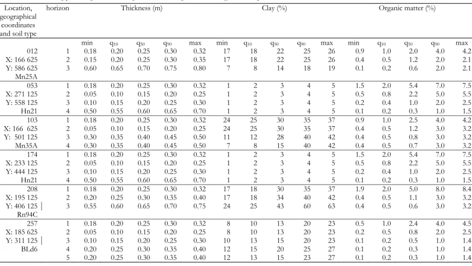
(36) Table 3.1. Parameters of probability distributions of soil thickness, clay content and organic matter for six selected locations. horizon Thickness (m) Clay (%) Location, geographical coordinates and soil type min q10 q50 q90 max min q10 q50 q90 max 012 1 0.18 0.20 0.25 0.30 0.32 17 18 22 25 26 X: 166 625 2 0.15 0.20 0.25 0.30 0.35 17 18 22 25 26 Y: 586 625 3 0.60 0.65 0.70 0.75 0.80 7 8 14 18 19 Mn25A 053 1 0.18 0.20 0.25 0.30 0.32 1 2 3 4 5 X: 271 125 2 0.05 0.10 0.15 0.20 0.25 1 2 3 4 5 Y: 558 125 3 0.10 0.15 0.20 0.25 0.30 1 2 3 4 5 Hn21 4 0.50 0.55 0.60 0.65 0.70 1 2 3 4 5 103 1 0.18 0.20 0.25 0.30 0.32 24 25 30 35 37 X: 166 625 2 0.05 0.10 0.15 0.20 0.25 24 25 30 35 37 Y: 501 125 3 0.30 0.35 0.40 0.45 0.50 11 12 28 40 42 Mn35A 4 0.30 0.35 0.40 0.45 0.50 7 8 15 40 42 174 1 0.18 0.20 0.25 0.30 0.32 1 2 3 4 5 X: 233 125 2 0.05 0.10 0.15 0.20 0.25 1 2 3 4 5 Y: 444 125 3 0.10 0.15 0.20 0.25 0.30 1 2 3 4 5 Hn21 4 0.50 0.55 0.60 0.65 0.70 1 2 3 4 5 208 1 0.18 0.20 0.25 0.30 0.32 17 18 30 35 37 X: 195 125 2 0.20 0.25 0.30 0.35 0.40 17 18 34 40 42 Y: 406 125 3 0.55 0.60 0.65 0.70 0.75 24 25 43 60 63 Rn94C 257 1 0.18 0.20 0.25 0.30 0.32 8 10 13 20 23 X: 185 625 2 0.05 0.10 0.15 0.20 0.25 8 10 13 20 23 Y: 311 125 3 0.10 0.15 0.20 0.25 0.30 10 13 15 20 23 BLd6 4 0.20 0.25 0.30 0.35 0.40 12 15 20 25 27 5 0.20 0.25 0.30 0.35 0.40 12 13 15 23 27. Alterra-report 1330. 35. Organic matter (%). min 0.9 0.4 0.1. q10 1.0 0.5 0.2. q50 2.0 1.2 0.6. q90 4.0 2.0 2.0. max 4.2 2.1 2.1. 1.5 0.5 0.2 0.1 0.9 0.4 0.4 0.4 1.5 0.5 0.2 0.1 1.9 0.4 0.4. 2.0 0.8 0.4 0.2 1.0 0.5 0.5 0.5 2.0 0.8 0.4 0.2 2.0 0.5 0.5. 5.4 2.2 1.0 0.3 2.5 1.2 0.8 0.7 5.4 2.2 1.0 0.3 5.0 1.1 0.6. 7.0 5.0 2.0 1.0 4.0 3.0 3.0 3.0 7.0 5.0 2.0 1.0 8.0 3.0 3.0. 7.5 5.5 2.5 1.5 4.2 3.2 3.2 3.2 7.5 5.5 2.5 1.5 8.4 3.2 3.2. 0.5 0.2 0.1 0.1 0.1. 1.0 0.5 0.2 0.2 0.2. 2.4 0.8 0.5 0.3 0.3. 4.0 2.0 1.0 1.0 1.0. 4.5 2.5 1.4 1.4 1.4.

(37) Table 3.2. Description of 36 building blocks and number of samples per building block analysed on soil hydraulic properties, before and after screening. Code top- or Description Nr samples Nr samples subsoil before retained after screening screening B01 top Loam-poor fine sand 32 32 B02 top Slightly loamy fine sand 27 27 B03 top Very loamy fine sand 14 14 B04 top Extremely loamy fine sand 9 9 B05 top Coarse sand 26 26 B06 top Glacial till 8 7 B07 top Sandy loam 6 6 B08 top Slightly sandy loam 43 34 B09 top Sandy clay loam 29 28 B10 top Clay loam 12 7 B11 top Heavy clay 13 2 B12 top Very heavy clay 9 2 B13 top Loam 10 10 B14 top Silty loam 67 55 B15 top Peaty sand 15 15 B16 top Sandy peat and peat 20 18 B17 top Peaty clay 25 17 B18 top Clayey peat 20 13 O01 sub Loam-poor fine sand 109 109 O02 sub Slightly loamy fine sand 14 14 O03 sub Very loamy fine sand 23 23 O04 sub Extremely loamy fine sand 9 9 O05 sub Coarse sand 17 17 O06 sub Glacial till 15 13 O07 sub Alluvial loam 15 12 O08 sub Sandy loam 14 14 O09 sub Slightly sandy loam 30 28 O10 sub Sandy clay loam 25 19 O11 sub Clay loam 11 7 O12 sub Heavy clay 25 14 O13 sub Very heavy clay 19 3 O14 sub Loam 9 9 O15 sub Silty loam 53 48 O16 sub Oligotrophic peat 16 15 O17 sub Eutrophic peat 36 36 O18 sub Weathered peat 7 5 Total 832 717. Recent analyses with SWAP (version 2.0.9) have shown that problems arise with some combinations of Mualem-van Genuchten parameters. Vanderborght et al. (2005) show that numerical problems occur when hydrology in soil profiles with soil and clay horizons are simulated with curves that have a very small value for the parameter n. In such cases SWAP (version 2.0.9) runs very slowly, may produce erroneous results or may even crash. Small values of the l and Ks parameters also give rise to problems. After careful screening it was therefore decided to remove all curves for which the parameter n was smaller than 1.1 (73 cases), or where the parameter l was smaller than -5.0 (40 cases) or where Ks was smaller than 0.01 (2 cases). In this way, extreme curves that did not fit in the corresponding building block were eliminated and the total number of 832 samples was reduced to 717. Two. 36. Alterra-report 1330.

(38) examples of Mualem-van Genuchten curves that did not pass the screening tests are given in Figure 3.4. The heterogeneity of the soil physical characteristics within a building block is also shown in Figure 3.4, where the distribution of Mualem-VanGenuchten curves of all individual samples of the B18 and O07 building blocks are presented. Other building blocks have similar results. It is clear from the large differences between the curves that soil hydraulic properties can markedly differ within building blocks. It is not only the variability within building blocks that determines the uncertainty about soil hydraulic properties. There is also uncertainty about which building block corresponds with each location and horizon. The building block is determined by entering the decision tree presented in Chapter 2 (see also Appendix 1). The way through the decision tree is partly determined by the basic soil properties of the location and horizon. Since these are uncertain, so is the building block. Table 3.3 gives the probability associated with the three most likely building blocks for all horizons of the six example locations. Note that the probability of the most likely building block varies between 0.31 and 1.00. Thus, uncertainty about basic soil properties causes a substantial uncertainty about what the building block at a location and horizon could be. However, alternative building blocks are typically ‘nearby’ building blocks that have similar behaviour, implying that the effect on soil physical properties may still be small. Note also that for all locations except location 257, uncertainty increases with increasing depth. Table 3.3. Three most probable building blocks with associated probability for all horizons of the six selected locations. location horizon First building block Second building block Third building block Code probability code probability code probability 12 1 B09 0.92 B10 0.05 B08 0.03 2 O10 0.88 O11 0.08 O09 0.04 3 O09 0.61 O08 0.31 O10 0.06 53 1 B02 0.85 B01 0.15 2 O02 0.54 O01 0.46 3 O02 0.57 O01 0.43 4 O01 0.59 O02 0.38 O03 0.02 103 1 B10 0.91 B11 0.05 B09 0.04 2 O11 0.87 O12 0.08 O10 0.05 3 O11 0.37 O10 0.30 O12 0.17 4 O09 0.31 O10 0.25 O08 0.24 174 1 B02 0.82 B01 0.18 2 O02 0.52 O01 0.48 3 O02 0.57 O01 0.43 4 O01 0.58 O02 0.40 208 1 B10 0.74 B09 0.17 B11 0.09 2 O11 0.55 O12 0.39 O10 0.07 3 O12 0.47 O11 0.29 O13 0.23 257 1 B14 0.94 B13 0.06 2 O15 0.94 O14 0.06 3 O15 1.00 4 O15 1.00 5 O15 0.95 O14 0.05. Alterra-report 1330. 37.

(39) c. a. d. b. Figure 3.4. Curves h(θ), and K(h) for two example building blocks B18 (left, a and b) and O07 (right, c and d). Solid grey lines are all curves that passed the screening, dashed red lines are example curves that did not pass the test.. 3.1.3 Stochastic simulation of uncertain soil properties The previous sections have explained how uncertainty in soil properties can be represented by probability distributions and how the parameters of these distributions were derived. This section discusses how samples can be generated from these distributions. Random samples are needed for the Monte Carlo uncertainty analysis discussed in the next chapter.. 38. Alterra-report 1330.

No results found