A MODEL OF THE
LOWER EXTREMITY BIOMECHANICS
DURING THE LUNGE
Joris De Roeck
Student number: 01506163Supervisors: Prof. Dr. Emmanuel Audenaert,
Dr. Jan Van Houcke
A dissertation submitted to Ghent University in partial fulfilment of the requirements for the degree of Master of Medicine in Medicine
A MODEL OF THE
LOWER EXTREMITY BIOMECHANICS
DURING THE LUNGE
Joris De Roeck
Student number: 01506163Supervisors: Prof. Dr. Emmanuel Audenaert,
Dr. Jan Van Houcke
A dissertation submitted to Ghent University in partial fulfilment of the requirements for the degree of Master of Medicine in Medicine
Deze pagina is niet beschikbaar omdat ze persoonsgegevens bevat.
Universiteitsbibliotheek Gent, 2021.
This page is not available because it contains personal information.
Ghent University, Library, 2021.
Preface
This project gave me the opportunity to analyze raw data from motion lab trials. I would like to thank Professor Dr. Emmanuel Audenaert for giving me the chance to discover how biomechanical data preprocessing, normalization and modelling works. I was able to develop different skills and to deal with several state-of-the-art software tools since I was responsible for the complete analysis of the lunge.
In the beginning, I spent a lot of time on getting to know this research field that was still unknown to me at that time. By applying secondary school mathematics in the MATLAB work environment, the data processing became more a learning process than a sequence of algorithms to achieve the intended results. Therefore, I experienced this like a diversion in the curriculum of the Master of Medicine, where I could be more involved in research.
Dr. Jan Van Houcke and ir. Diogo Almeida kickstarted me for the first data processing. I compared several times my data proceedings with the intermediate results from Diogo’s deep squat analysis. These short moments were very helpful. Professor Dr. Audenaert was also available in case of any problems. I am obviously grateful to them. In the course of time, I was able to do data processing entirely on my own.
In addition, I would also like to express my thanks to my brother, Lieven. He has a more mathematical background and it was fine to discuss several data processing related issues with him. He also taught basic skills from computer programming. Next to it, there were some YouTube channels that helped me out of confusion many times.
Furthermore, I insist on thanking all participants and collaborators from the motion lab study. Without them, none of this would have been possible. The study was part of a PhD project by Dr. Jan Van Houcke. Finally, I sincerely hope that you, as a reader, will get a clear understanding from model development to model interpretation as you go through my work.
Table of contents
Abstract ... 1
Abstract in Dutch ... 2
1 Introduction and research question ... 4
1.1 Surgery planning ... 4
1.2 Exploring the lower limbs biomechanics ... 4
1.2.1 The lunge ... 6
1.2.2 The mechanisms behind joint reaction forces ... 7
1.2.2.1 The hip ... 7
1.2.2.2 The knee ...11
1.2.2.3 The ankle ...12
1.3 Pathological phenomena due to loading aberrations ...12
1.3.1 The role of cartilage...12
1.3.2 Hip pathology ...13
1.3.2.1 Femoroacetabular impingement ...13
1.3.2.2 Hip osteoarthritis ...15
1.3.2.3 Active shape modeling ...16
1.3.3 Knee pathology ...16
1.3.4 Ankle pathology ...17
1.4 Hypothesis and aim of the study...17
2 Methodology ...19
2.1 Study sample ...21
2.2 Motion lab analysis ...22
2.3 Computer simulation in a musculoskeletal model ...23
2.4 Creating a statistical model ...24
2.5 Model validation ...26
2.5.1 Model accuracy...26
2.5.3 Model generalization ...26
2.5.4 Model specificity ...27
3 Results ...28
3.1 The kinematic model of the lower limbs during lunge ...28
3.2 Validation results ...32
4 Discussion ...37
4.1 Description of the modes ...37
4.2 Final considerations ...39
5 Reference list ...41
6 Attachments ...44
6.1 Appendix 1: Marker trajectory editing in Motive ...44
6.2 Appendix 2: Working in the Anybody Modeling System ...44
List of figures
Figure 1. Knee load before and after menisci resection in the frontal and sagittal plane. Figure 2. Sketch from the lower limbs during different lunge tasks.
Figure 3. A static force body diagram of a frontal plane of the right hip while standing up. Figure 4. Influence of the CCD angle or neck-shaft angle on the abduction force.
Figure 5. The measurements of the acetabular and femoral version angle Figure 6. The teardrop sign.
Figure 7. Illustration of the α and β angle, as well as the anterior and posterior offset.
Figure 8. An illustration of the CEA and AI on X-ray in anteroposterior view Figure 9. A static force body diagram of the knee joint.
Figure 10. Sagittal sections of the hip joint during flexion.
Figure 11. Cartilage injury distribution in isolated pincer and cam-type FAI. Figure 12. Illustration of the general work flow.
Figure 13. Flow chart of the raw data processing.
Figure 14. Scree plot with the cumulative variance of the modes (or PCs) capturing the
training data.
Figure 15. Variance of the first mode relative to the training data.
Figure 16. Graphical representation of the variance described by the first component. Figure 17. Variance of the second mode relative to the training data.
Figure 18. Graphical representation of the variance described by the second component. Figure 19. Variance of the third mode relative to the training data.
Figure 20. Graphical representation of the variance described by the third component.
Figure 21. RMSE for the original training data versus the reconstructed data from models with
an increasing number of PCs.
Figure 22. Accuracy evolution of waveform data for different levels of prior knowledge
expressed as amounts of training data in a kinematic model and the in-sample target accuracy.
List of tables
Table 1. Demographic and anthropometric characteristics of the study population. Table 2. Validation analysis of the kinematic model.
List of abbreviations
AI Acetabular index
AMS Anybody Modeling System
APT Anterior pelvis tilt
ASM Active shape model
BMI Body mass index
BW Body weight
CCD Caput-collum-diaphyseal
CEA Center edge angle
CSV Comma-separated values (raw data file extension)
CT Computed tomography
CTX-II C-terminal cross-linked telopeptide type II collagen
ECM Extracellular matrix
FAI Femoroacetabular impingement
GAG Glycosaminoglycans
HJRF Hip joint reaction force KJRF Knee joint reaction force mJSW Minimal joint space width
MoCap Motion capture
MRI Magnetic resonance imaging
PC(s) Principal component(s) PCA Principal component analysis
PCHIP Piecewise Cubic Hermite Interpolating Polynomial
RMSE Root-mean-square error
ROM Range of motion
STL SurfaceTessellationLanguage or StandardTessellationLanguage (stereolithografie file extension)
Abstract
Purpose – Modern statistics and higher computational power have opened novel possibilities
to complex data analysis. While gait has been the outmost described motion in quantitative human motion analysis, descriptions of more challenging movements like the lunge are currently lacking in the literature. By linearly combining the variance of kinematic data like flexion angles, a biomechanical model of the lower extremities can be created. This way, lower limb data is considered as a whole and not described by deduced spatiotemporal parameters like maximum flexion or stride length, as done in many gait analyses, resulting in huge loss of waveform data. The hip and knee joints are exposed to high forces and cause high morbidity and costs. Up to now, targeted prevention is lacking due to the absence of appropriate biomarkers or specific radiological markers to detect damage at an early stage. Since osteoarthritis is a disease that usually develops very slow, where compensation mechanisms become no longer sufficient, motion lab analysis will provide an endless source of information in the future. Other applications can be found in sports, surgical planning, implant designs, prediction of cognitive decline, disability monitoring and so on.
Methods – Lunge trials were performed by healthy Caucasian male (n=53) without overweight
and approximately the same age and activity level. Based on the limited population studied here, it is expected that the variance can be described simply. Musculoskeletal model simulations were executed in the Anybody Modeling System based on subject-specific geometry and the state-of-the-art TLEM 2.0 dataset. Principal component analysis is applied as a dimensionality reduction technique in order to enable variance decomposition. This current paper is, to the author’s knowledge, the first to investigate generalization of kinematic model data towards the population. Out-of-sample accuracy is explored by reconstructing data for one of the test subjects based on new models created by a subset of other training data. Finally, model specificity is investigated by generating new test data from the model.
Results – The obtained statistical model proved to be accurate and compact as merely 9 (out
of 52) principal components account for 95% of the total population inter-individual variability and is able to reproduce the original data with a median root-mean-squared error below 0,1344°. The specificity was similar as when considering 90% or 98% variance, while the RMSE for in-sample accuracy is lower at higher variance, as expected.
Conclusion – Regarding a population with cases of impingement or osteoarthritis, elderly
people and other distinguishing features, lunges are supposed to be performed in many different other phenotypes because there is not a consistent way to do this in the normal population. For models aimed at population covering descriptive studies, the number of training samples required must be at least 30.
Abstract in Dutch
Probleemstelling – Moderne statistiek en de hoge computerkracht openen nieuwe
mogelijkheden voor complexe data-analyse. Terwijl het stappatroon veruit de meest onderzochte beweging is in kwantitatieve bewegingslabo analyse (cf. de term ganglabo), is er geen evidentie over de beschrijving van meer uitdagende bewegingen zoals de lunge. Een biomechanisch model van de onderste ledematen kan bestaan uit het lineair combineren van variantie van kinematische data. Op deze manier worden de onderste ledematen in hun geheel beschouwd en niet door afgeleide parameters die ruimte en tijd beschrijven, zoals maximale flexie of paslengte. Helaas wordt dit wel gedaan in vele ganganalyses, wat resulteert in een enorm verlies van potentieel relevante data. Het heup- en het kniegewricht worden blootgesteld aan hoge belasting en zijn belangrijke oorzaken van morbiditeit, wat veel kosten met zich meebrengt. Tot nu toe is er geen specifieke preventie omdat er geen (radiologische) merkers bestaan die aan de voorwaarde van een goede biomerker voldoen om schade in een gewricht vroegtijdig te detecteren. Vanwege het sluipend karakter van osteoartrose, waarbij compensatiemechanismen na verloop van tijd meer en meer tekortschieten, zouden bewegingslabo’s een onuitputtelijke bron van informatie kunnen verschaffen. Andere toepassingen zijn terug te vinden bij sport, chirurgische planning in het kader van computerondersteunde chirurgie, de vorm van prothesen, voorspelling van cognitieve achteruitgang, invaliditeit, overleving, enzovoort.
Methodologie – Lunge bewegingen werden uitgevoerd door gezonde, jonge mannen van het
Kaukasisch ras (n=53) met een BMI-index tussen 18,5 en 25. De variabiliteit van de bestudeerde populatie werd zo beperkt mogelijk gehouden doordat de vrijwilligers bij benadering dezelfde leeftijd en activiteitsniveau hadden. Bijgevolg werd er verwacht dat de variantie eenvoudig beschreven zou kunnen worden. In Anybody werden er simulaties gedaan op basis van modellen die gebaseerd zijn op de geïndividualiseerde botmorfologie en de geavanceerde TLEM 2.0 dataset. Als dimensionaliteitsreductietechniek werd principale-componentenanalyse toegepast met als doel de variantie te ontleden. Volgens de auteur is dit het eerste werk dat de generaliseerbaarheid van modellering met kinematische data ten opzichte van de populatie nagaat. Accuraatheid buiten de steekproeven werd onderzocht door data te reconstrueren op basis van nieuwe modellen die gebaseerd zijn op een subset van andere data uit de originele steekproef. De model specificifiteit werd onderzocht door nieuwe data te genereren vanuit het model.
Resultaten – Het model is voldoende accuraat en compact omdat 95% van de variantie uit de
bedraagt. De specificiteit was gelijkaardig voor modellen met 90% en 98% variantie. Zoals verwacht was de de accuraatheid beter bij toenemende variantie.
Besluit – Betreffende een populatie die bestaat uit personen met impingement, osteoartrose,
oudere personen en andere diverse kenmerken, zullen de lunge bewegingstrajecten met nog meer verscheidenheid uitgevoerd worden. Dit is te verklaren omdat er binnen een scherp afgelijnde populatie reeds geen consistente manier bestaat om de lunge uit te voeren. Om in toekomstige studies de populatie voldoende te dekken met statistische modellen, bedraagt het minimaal aantal vereiste proefpersonen 30.
1 Introduction and research question
1.1
Surgery planning
Total knee replacement (TKA) and total hip replacement (THA) are two of the most common surgeries performed today. Both operations aim to relieve pain, but in short term a lot of post-operative pain has been observed (1). The fear of acute pain has been cited as the reason why arthritic patients delay arthroplasty surgery to a further stage with more complications (1, 2). Despite good treatment modalities for painful complications like trochanteric bursitis, pain is the major component that determines patient satisfaction (1, 3). Nowadays, trochanteric bursitis is even used as an umbrella term encompassing different pathologies known to cause lateral sided hip pain because there are no standardized criteria for diagnosis (3).
There is an apparent need for accurate surgical planning for TKA and THA. Next to the importance of (preemptive) analgesia, the choice of a custom-made prosthesis would affect the pain sensation. Joint loadings would induce pain stimuli. A better understanding of the lower limb biomechanics could lead to more personalized prostheses with less pain by reducing the focal peak load.
In 1870, a German surgeon, called Julius Wolff, pioneered the mother of all bone laws, stating that bone adapts to the load it is exposed to (4). Subtle bone morphology variations are measurable by magnetic resonance imaging (MRI) and they are assumed to be a consequence of load distribution. Excessive load is considered to be a risk factor for hip osteoarthritis, which is probably underdiagnosed (5).
1.2
Exploring the lower limbs biomechanics
The kinetics is concerned with the relationship between forces and their effects on motion. Joint forces and torques arise because people are liable to gravitation that can be dominated by muscle use. These are quantities to assess inertia. By contrast, the kinematics describes the motion of points or objects without concerning the cause of motion, in terms of position (angles) and its first and second derivatives, respectively the velocity and acceleration (6). There are several ways to examine lower limb biomechanics. Motion can be detected by X-ray fluoroscopy or in a motion lab. The purpose of fluoroscopy is to determine the longevity of prostheses that is limited by aseptic loosening and component wear. In vivo measurements are gauged by instrumented hip or tibial implants, that is only available for a limited number of subjects after surgery. These findings cannot be extrapolated to the general population (7-10). The remaining option is to investigate intern forces in silico, i.e. by simulating them in subject-specific computer models. Several packages, like the open source Opensim or commercial
packages like SIMM/FIT, BRGLifemodeler and the Anybody Modeling System (AMS) are available to do so (4, 7, 11).
To predict the forces inside joints, computer simulation models shall use a so-called inverse dynamics approach. Therefore, the outside forces are measured to get an idea of the forces inside the human body. Quantitative kinetic analysis can be based on walking (gait), various sitting positions, as well as specific movements like cycling, deep squatting and lunging, which are more demanding exercises (12-14). Humans use a similar range of motion (ROM) during their daily activities, so research into the lunge will give an impression of the inside forces during live.
Concerning the lower limbs, there are three joints on each side except from the different articulations in the foot inside. The hip or the acetabulofemoral joint is spheroid, although there is some measurable incongruity (6, 15-17). The knee is the largest joint in the human body. It is defined as a modified hinge joint that consists of the tibiofemoral and the patellofemoral joint. The cruciate ligaments and menisci act as a loading transfer medium. If the menisci are removed, the knee load will be three times higher, as figure 1 suggests. Finally, the ankle is considered as a less typical hinge joint because it allows a limited degree of rotation or side-to-side movement in dorsal flexion (6, 17). On the other hand, it is a joint that is surprisingly flexible among experienced ballet dancers (6).
Figure 1. Knee load before and after menisci resection in the frontal (A) and sagittal plane (B).
Inter- and intrapersonal variability can result in excessive and disproportionate joint loadings, on the place where adjacent bone surfaces meet each other. It could be related to osteoarthritis: a highly prevalent form of arthritis in the western world that often occurs in large weight-bearing joints (18). It is supposed to be the most common musculoskeletal disorder worldwide (19). Variations in bone anatomy, like femoroacetabular impingement (FAI), would accelerate the disease progression. Also, different functional activities performed during work
anatomy inside through cartilage and subchondral bone degeneration and osteophyte generation (20). The hyaline cartilage is a load bearing surface, that protects the end of the bones because of its resilient properties (21, 22).
1.2.1 The lunge
The lunge is often applied during muscle stretching in training and rehabilitation exercises and also in common daily activities and sports like badminton, squash and fencing (6, 13, 23-25). In these sports, footwork techniques are crucial to enable to move quickly into the best possible position and to return to the base position to prepare for the opponent’s return action (24). The task essentially consists of a weight acceptance phase (braking) and a rapid accelerating phase (recovery) (13). Unfortunately, there is currently a lack of evidence on the mechanics of this advanced movement skill available in literature.
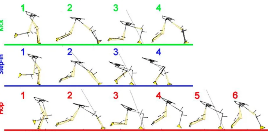
Kuntze et al. investigated different lunge tasks among student badminton players. The way to do lunging may influence muscular fatigue and the injury risk potential (13). Three traditional lunge tasks are chalked out in figure 2. Here, the test subjects performed a standard, kick lunge step.
Figure 2. Sketch from the lower limbs during different lunge tasks: the kick (green), step-in (blue) and
hop (red) exercises (adapted from Kuntze et al.) (13).
Qichang et al. demonstrated higher peak pressures on the lateral parts of the foot among recreational badminton players compared to elite badminton athletes. Conversely, peak pressures on the medial metatarsus and hallux were lower. Differences in hip flexion, knee adduction and internal rotation of the knee were also observed. It suggests other joint reaction forces and muscle activation patterns in higher-level players. This knowledge may be useful to instruct amateur players (24).
1.2.2 The mechanisms behind joint reaction forces
Reaction forces are the reflection of gravity and additional muscle forces that balances the body. Gravitation can be eliminated by the Archimedes’ principle of buoyancy. This idea is widely used by top athletes during aquatic-based rehabilitation programs to regain mobility, muscle strength and cardiovascular endurance without aggravating their injury (26).
1.2.2.1 The hip
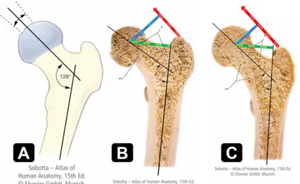
The hip is an outstanding example to explain the stabilizing function of muscles, resulting in higher joint forces than you may expect on the basis of gravity alone. Figure 3 illustrates the the hip joint reaction force (HJRF) in the frontal plane. A large moment arm of the gravity and a small moment arm of the abduction force cause a huge reaction force in the hip joint. The gravity force is proportional to the body mass but does not comprise legs and feet. These torques will vary among different individuals. The HJRF is up to a fourth lower in the coxa vara configuration, whereas it is a quarter higher than normal in coxa valga (27). The mechanism behind this is explained in figure 4.
Figure 3. A static force body diagram in the frontal plane of the right hip while standing up. or is the weight or gravitation force lying on the gravity line of the subject (if the lower limbs are not included). is the adduction force, neutralized by the abduction muscles force or , so . pulls along the trajectory of the gluteus medius and minimus muscle fibers. represents the HJRF. The center of the femoral head acts as a center of rotation of the moment arms, like a lever arm.
Analogously to the abductor moment, there exists also a flexion and rotation moment, respectively in the sagittal and transverse plane. The HJRF depends on the position of the gravity line. Schwab et al. found that for young adults, the femoral head position appears to be a reliable radiographic indicator of the gravity line in the sagittal plane (27). This means that during standing upright, the flexion or extension torques will very slightly contribute to the total HJRF.
Figure 4 illustrates the differences in moment arms of the small gluteal muscles depending on the neck-shaft angle (28). At the epiphyses, being the articular ends of long pipe bones, there is mainly cancellous or spongy bone encompassing the trabeculae. The lateral part of the femur neck consists of a horizontally oriented network of trabeculae trajectories due to traction, while the medial low-lying part has a vertically oriented web of trabeculae because of compression. This is a typical example of the bone law by Julius Wolff (4).
Contrary to the moment arm, the femoral offset is commonly used in THA jargon. It refers to the perpendicular distance from the femur shaft axis to the rotation center of the femoral head (4). The version angles (figures 5 and 6) can interfere and are described further in this section.
Figure 4. Influence of the caput-collum-diaphyseal angle (CCD angle) or neck-shaft angle on the
abduction force (adapted from Sobotta et al.) (28). (A) Normal proximal femur configuration in an adult. (B) A low normal CCD angle of 120 degrees (borderline coxa vara). Increased traction forces cause a reinforcement of the lateral cancellous bone (*) and a reduction of the medial bone (**). There is an enlarged moment arm, as there is an increased femoral offset, resulting in lower muscle abductor forces and therefore, also lower joint reaction forces. (C) A high normal CCD angle of 130 degrees. Here, there is a high amount of the medial cancellous bone (**) due to compression , unlike a reduction on the lateral side (*). The femoral offset is smaller than in (B), so the HJRF will be relatively higher.
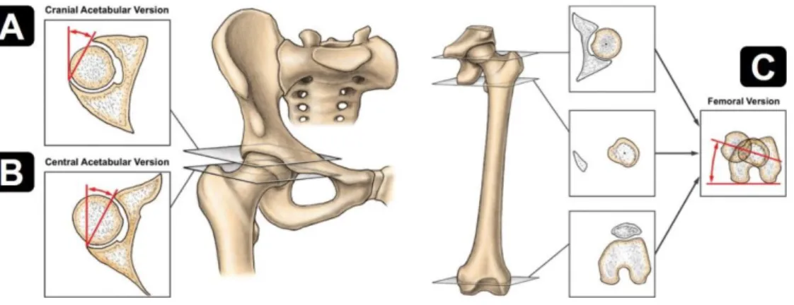
Figure 5. The measurements of the acetabular (A+B) and femoral (C) version angle (from Lerch et al.)
(29).
The acetabular cup location and cup abduction are objectified by the acetabular offset and the cup abduction angle. They also determine the forces on the hip. The acetabular offset is the shortest distance between the acetabular rotation center and the perpendicular to the interteardrop line through the teardrop. The interteardrop line is the line from the left to the right teardrop on X-ray (4). The acetabular teardrop is a U-shaped density taken in anteroposterior projection, as shown in figure 6 (30). The offset and abduction angle determine the upper anterior weight bearing area of the hip joint that should be large enough to distribute the load. Additionally, posteroinferior acetabular coverage is necessary to stabilize the joint. The shorter the acetabular offset, the longer the femoral offset and the lower the total HJRF.
Figure 6. The teardrop sign (from Dandachli et al.) (31).
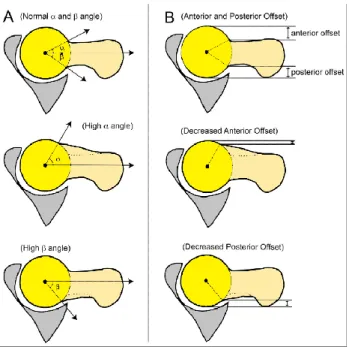
Other anthropometric measurements are the alpha angle, center edge angle and will be measured for each volunteer as in table 1 in the methodology section. The alpha angle is the angle formed by the femoral neck axis and a line connecting the center of the femoral head with the point at the beginning of sphericity, as showed in figure 7 (32). Clinical trials have shown a correlation between the alpha angle and cartilage defects within the hip joint (5).
Figure 7. Illustration of the α and β angle, as well as the anterior and posterior offset. This figure shows
the variety in femoral head-neck configuration (from Amanatullah et al.) (33).
The center edge angle (CEA), as showed in figure 8, is the angle formed by a line parallel to the longitudinal pelvic axis and the line connecting the center of the femoral head with the lateral edge of the acetabulum. The center edge angle, CCD angle, femoral anteversion, or acetabular anteversion were not found to differ between certain groups. The lateral center edge angle and alpha angle would predict the risk of THA independently, however another study concluded that the CEA does not differ in (asymptomatic) cam patients compared to healthy controls. The CEA describes pincer morphology (cf. figure 10) (32, 34).
Figure 8. An illustration of the center edge angle (CEA) and acetabular index (AI) on X-ray in
anteroposterior view (from Ghaffari et al.) (15). The line with indication 5 is drawed between the medial and lateral margins of the sourcil impression on X ray.
Finally, the AI (see figure 8) is the angle of the sourcil relative to the inferior pubic rami axis (35). The CCD angle and the femoral and acetabular version angles are mentioned in figures 4 and 5. Higher femoral or acetabular version angles are associated with more internal rotation
during running to prevent luxation (6). As such, in the case of a cam-type impingement (see section 1.3.2.1), the femoral and acetabular version angle will be associated with more abutments.
At last, there are many other radiologic parameters that can be deduced from imaging of the bone geometry, like the minimal joint space width (mJSW), that are not stated here (35-37). Morphological points can be combined in a shape model, as explained in section 1.3.2.3. These principles are used in THA with the purpose to advance prosthesis durability and convenience. However, a prosthesis with an excessive femoral offset can lead to increased micromotion at the implant bone interface, leading to overload and associated pain (4). However, the presumed correlation between trochanteric bursitis and an excessive offset has not yet been proven (3). On the other hand, less tension can lead to instability. To enable a maximal impingement-free ROM, the femoral anteversion and the acetabulum configuration must be evaluated too (4).
During the open kinetic chain parts of the right-forward lunge, a discreet unipedal stance occurs. This means that one leg is wearing the whole body weight for a while. In the young adult population, the gravity line lies anterior to the spine in the midsagittal plane (27). So, while standing on a single leg, the gravity will cause a substantially increased adduction moment of the supported leg. Hip abductor muscles like the Mm. glutei medius et minimus, also called the small gluteal muscles, stabilize and prevent tilting of the pelvis to the contralateral side (28).
1.2.2.2 The knee
Figure 9 illustrates a simplification of the forces in a relaxed bended knee. The result force is zero, so the object remains at rest, as proposed by the first Newton’s law of motion. Concerning a motion, these forces will not counterbalance each other. As formulated in the second Newton’s law, the object will accelerate with a linear acceleration a or angular acceleration resulting in a force F or a moment M where J acts as moment of inertia (unit: kg m²).
or
The tibiofemoral knee joint reaction force (KJRF) exerts pressure on the tibial condyles. As mentioned in the third Newton’s law, this force will be equal in magnitude but opposite in direction compared to the force on the femoral condyles (6).
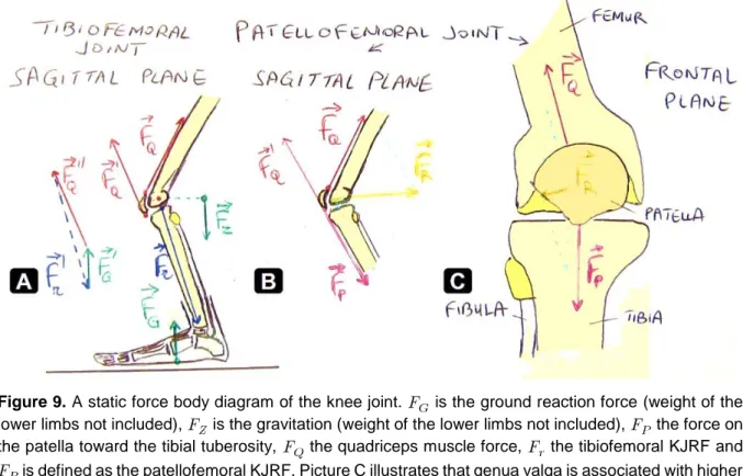
Figure 9. A static force body diagram of the knee joint. is the ground reaction force (weight of the lower limbs not included), is the gravitation (weight of the lower limbs not included), the force on the patella toward the tibial tuberosity, the quadriceps muscle force, the tibiofemoral KJRF and is defined as the patellofemoral KJRF. Picture C illustrates that genua valga is associated with higher lateral compression forces in the femoral trochlear groove (6, 17). Notice that the quadriceps muscle is the only extensor of the knee (17).
The presence of a patella is of vital importance regarding the KJRF. Its function is to enlarge the lever arm of the knee joint, especially during deep flexion, associated with a peak reaction force in the patellofemoral joint. The KJRF will be higher after resection of the patella. In that case, there will be an enlarged quadriceps muscle force, but the torque remains the same (6, 17).
In contrast to what Galloway et al. did for gait, it could be useful to integrate knee biomechanics into a model that considers the entire lower limbs. This seems intuitively justified because all knee muscles are biarticular, except for the M. popliteus (17, 28, 38).
1.2.2.3 The ankle
Like the knee, the ankle is not very mobile because of its important stabilizing properties, especially in dorsiflexion (17). In this study, only the tibiotalar joint will be considered.
1.3
Pathological phenomena due to loading aberrations
1.3.1 The role of cartilage
Subchondral bone is covered by a hyaline cartilage layer. It consists of an extracellular matrix (ECM) composed of proteoglycans, collagen fibers and a low density of chondrocytes (15). Proteoglycans are secreted or attached to cell-surface glycoproteins with covalently linked
polysaccharide chains, also called glycosaminoglycans (GAG). They are crucial in the cell-ECM adhesion. One of them is hyaluronan, a major component in the cell-ECM. This non-sulfated GAG is the backbone of proteoglycan aggregates. Due to anionic residues on hyaluronan surfaces, the molecules bind large amounts of water, forming a kind of hydrated gel. If the pressure increases, hyaluronic molecules will tend to push outward, creating a turgor pressure. That swelling gives the connective tissues the ability to resist compression, in contrast to collagen II fibers that can resist stretching forces by providing the tensile and shear strength in cartilage (15, 22, 39).
Early stages of cartilage injuries are characterized by increased water content, disruption of the collagen network and loss of glycosaminoglycans. The histologic injury will lead to changes that are detectable on T1- and T2-weighted MRI. Fat-suppressed T1 images provide better contrast between cartilage and surrounding tissues, while non-fat suppressed images permits higher spatial resolution (39). Moderate-to-severe cartilage injuries may be a contraindication to joint preservation surgery (15).
1.3.2 Hip pathology
1.3.2.1 Femoroacetabular impingement
FAI is characterized by early and repetitive abutments between the acetabular rim and the proximal femur (which is the femoral head and neck), resulting in concomitant damage in the conflict area, as delineated in figure 11. Abutments occur during full flexion and internal rotation, usually caused by an osseous malformation on the subchondral parts of the bone (2, 5, 15). It is a common cause of hip pain and limited range of motion
in young and middle-aged adults (2, 5). Impingement pain is typically located in the groin or great trochanteric region and typically extends to the lateral side of the thigh (32).
Malformations are categorized in terms of cam and pincer impingement. They are presented in figure 10. The mixed-type is the most common form of FAI, where both cam and pincer morphologies exist (2, 15). Each deformity would be present in about one in three asymptomatic men (15).
FAI can occur with normal osseous anatomy, which is typically of gymnasts with joint hypermobility and excessive training. The prevalence among adult athletes is estimated at more than a half (40). Pincer and cam lesions are usually idiopathic in etiology (2). Hence, radiologists should routinely assess for FAI morphology on all pelvic radiographs without evidence of moderate-to-advance osteoarthritis. Checklist approaches are available to allow radiologists to detect efficiently subtle image findings of FAI and to classify them. Some institutions even perform magnetic resonance arthrography (MRA) while pulling the legs.
During this so-called termed traction arthrography, the contrast dye would penetrate the joint better, to make the distinction between the cartilage and bone easier (15).
Figure 10. Sagittal sections of the hip joint during flexion. (A) A normal hip during standing upright. (B)
A normal hip where the maximal flexion of 90 degrees is reached without abutment of the labrum with the femoral neck [1]. (C) A hip with a kind of pincer-type morphology showing anterior osseous acetabular over-coverage [2], causing premature labral wear [3]. Accordingly, further flexion is avoided by the interaction between the femoral neck and the thin rim on the edge of the acetabular cartilage [4]. There is also a vulnerable load occurring on the posterior side of the joint due to the resultant hip reaction force that holds the leg in flexion, accompanied by a slight subluxation. This typically creates contre-coup lesions [5]. Also, other manifestations like acetabular retroversion can pose as a pincer-type impingement. (D) A hip with cam-type morphology showing an osseous antero-lateral prominence, which is the most commonly occurrence of this deformity [6]. This bone protrusion causes shear stresses between the deep layer of acetabular cartilage and subchondral bone. The subsequent cartilage delamination may develop a cartilage flap [7]. Here, the labrum is somewhat displaced but still intact and fixed to the underlying subchondral bone [8] (from Ghaffari A et al.) (15).
The pincer-type impingement can cause labral tears and degeneration during hip flexion and internal rotation, by compressing the labrum to the acetabular subchondral plate. The labrum is the structure enlarging the acetabular cup. This cartilage ring can be completely absent in long-standing FAI or osteoarthritis. There are different patterns of pincer proliferation that would be important for further policy (15).
A cam-type impingement is associated with high-impact sporting activities during skeletal maturation (41, 42). There is an increased contact pressure on the acetabular cartilage upon intrusion of the prominence during flexion, abduction and/or internal rotation. Neutral internal rotation would not provoke cam intrusion (5). Coxa vara could cause cam-type impingements due to the altered neck-shaft angle. However, the magnitude of the reaction force will be lower, owing to the change in length of the abductor level arm (4, 15). During full hip flexion, such as in low car seats, the anterior femoral neck protuberance will touch the acetabular cartilage in the anterosuperior quadrant on the edge of the hip bowl (5, 12, 15). It drives the cartilage centrally and the labrum peripherally, so it could cause chondrolabral separation (15).
Audenaert et al. found differences in the pattern of cam engagement among patients with cam-type impingements during flexion, abduction and internal rotation in 90° of flexion, which is probably the most relevant motion. Anyway, all motions causing cam intrusions appeared to focus on the same cartilage area. This finding suggests that only complete resection of the femoral conflict area will prevent further damage (5). FAI is likely to be the primary contributor to idiopathic hip osteoarthritis (15).
Figure 11. Cartilage injury distribution in isolated pincer (C) and cam-type FAI (D). Notice the applied
clock-face orientations (A and B) (from Siebenrock KA et al. and Ghaffari A et al.) (15, 41).
1.3.2.2 Hip osteoarthritis
Kopec and colleagues suggest that ethnicity influences osteoarthritis dependent of the joint and stage of the disease according to the Kellgren and Lawrence classification system. This is a method of classifying the severity of osteoarthritis in the spine, hip, knees and so on by using five grades (18, 43). Progression of knee osteoarthritis is higher in African Americans compared to whites. However, African American are less predestined to develop hip osteoarthritis. Differences in joint anatomy and biomechanics, physical activity, muscle strength and other factors might explain these differences (18).
Symptomatic osteoarthritis patients can benefit from conservative interventions, intra-articular injections of glucocorticoids and hyaluronic acid as well as opioids in severe cases as used for acute postoperative pain (1, 2). Drug treatment does not affect the progression (44). If the pain causing limitation of activity persists, hip preservation surgery will be considered if there are no contraindications like advanced chondral damage. Postponing a treatment on behalf of a lack of diagnostic tools will result in end-stage disease with more sequels and poor outcomes after the appropriate therapies.
Precautionary treatment in asymptomatic patients is still controversial (2). This should be considered as it may affect disease progression in the early stages (15). Furthermore, FAI also
computed tomography is not suitable to do so, which is the major reason why computed tomography (CT) scanning is less appropriate to examine FAI (15).
1.3.2.3 Active shape modeling
As a PhD project, Almeida (University of Ghent, Belgium and University of Lisbon, Portugal) developed an active shape model (ASM) of the femur geometry based on X-ray CT scans to improve arthroplasty planning. Active shape modeling is a way of fitting images or virtual three-dimensional objects in a model by Procrustes analyses and principal component analysis (PCA) (19). ASM uses landmark points to describe the object outline. Each landmark refers to the same location, allowing variation in shape that can be measured across two-dimensional X-rays as well as three-dimensional structures with virtual reconstructed bones after CT segmentation. Here, different descriptors for osteoarthritis with low sensitivity and specificity were replaced by a model with modes describing the overall bone morphology variation as a new, reliable and predictive biomarker, independent of the radiologist interpretation (37). Furthermore, awareness of race and gender differences is recommended. Nelson at al. found higher alpha angles, greater mJSW and AI in male, among other things. Their findings also suggested that African Americans would have a narrower pelvis compared to whites (35).
1.3.3 Knee pathology
Osteoarthritis mostly affects the knee joint (14). Knee arthritis is a heterogeneous condition characterized by changes in a variety of joint tissues with discordant biomechanical features (45, 46). It has a huge impact on daily, recreational and professional live.
Many studies observed that loss of the anterior cruciate ligament is associated with gait and movement asymmetries as well as changes in knee joint loadings (14, 44). Also knee extensor weakness is associated with gonarthritis (44). A balanced muscle function seems to be essential for the knee joint. Furthermore, there are classical risk factors like obesity, ageing, genetic traits, malalignment, previous knee injuries and pain at baseline. There is poor level of evidence about self-management treatment (44, 45).
Meireless et al. showed that in early stages of knee osteoarthritis, altered knee loading of the cartilage on the medial tibia plateau was found, by using a musculoskeletal model that calculates the compartmental joint loading (24). Take notice that the medial tibial condyle is one and a half times as large as the lateral one (6). If the normal load bearing contact changes to a region less predisposed, there is a higher risk for degenerative damage. Peak knee rotation moments were different between patients with early osteoarthritis and controls during the stance phase of the step-up-and-over exercise. This reveals that the knee rotation moment should receive more attention in literature instead of the knee flexion moment only (24).
Knoop et al. investigated the link between knee OA, tissue abnormalities and biomechanical factors. They found, among other things, an association of cartilage integrity with quadriceps weakness and reduced laxity in knee varus and valgus (46).
Biomechanical parameters could be integrated in a machine learning approach for phenotyping knee osteoarthritis and progression, together with other variables like urine CTX-II (C-terminal cross-linked telopeptide type CTX-II collagen). It has been proven that this waste product of cartilage is the most consistent biomarker of knee OA progression available nowadays (45).
1.3.4 Ankle pathology
In contrast to hip and knee, cartilage lesions in the ankle are often a complication of fractures (17). As in the hip and shoulder, impingement syndromes in the ankle are an increasingly recognized source of pain. Impingements in the ankle include a spectrum of pathologies involving both osseous and soft tissue abnormalities. There is no classification, but pathologies are traditionally divided into anterior and posterior impingement syndromes for simplicity. Anterior impingement occurs with dorsiflexion at the front of the ankle joint like during deep squatting, while the opposite is true for the posterior variant as in the case of wearing high heels. The latter can be confused with Achilles tendinopathy. Both forms have been demonstrated in athletes and elite dancers (47). There is little literature available on this topic.
1.4
Hypothesis and aim of the study
Movements are the result of cognitive control involving attention, planning, memory and other motor, perceptual and cognitive processes (8, 11, 14, 26, 44, 46, 48). Morphological variations and deformities are at the basis of limited ROM (4, 5, 29). In this study, the relationship of the variance in kinematics from the lower extremities will be investigated by creating a statistical model.
Many motion analyses studied anthropometric, spatiotemporal, kinematic and kinetic parameters for gait analysis. Gait tests do not focus on higher hip flexion, where bone and cartilage collisions may occur. Because of the lack of evidence available for the lunge, this study only considers the normal occurrence in the population, where each field of investigation starts. There is growing evidence that human movement analysis provides more information about cardiovascular disease, disability and survival (48). For example, in the Rotterdam study, Lahousse et al. found that FEV1 is significantly associated with stride time and stride length (49).
Research in healthy biomechanical patterns like for the lunge is important to determine what is normal. Because of the huge amount of waveform data when investigating a patient,
variances make it difficult to categorize and diagnose what is pathologically (48). New diagnostic tool could be very important in orthopedics, where usually prevention is only done when the damage is already very large. Perhaps, current surgery does not always solve the causal problem, that can be objectified by a kinematic investigation, leading to relapses. Also for monitoring, lunge motion labs could be useful because with the diagnostic tools nowadays, it is doubtful whether asymptomatic patients having radiologic findings of impingement should undergo more stringent preclinical monitoring (32).
To eliminate age-related, sex-related and other potential causes of variation, the subjects here investigated will be homogeneous. This type of data is probably more meaningful and less surrogate than bone geometry, to assess (subliminal) damage and risk factors for hip and knee pathology, that are often associated with each other. MRI and CT scans only show consequences of damage but not the causes and hence, there are many false negatives and false positives. For example, maybe the patellofemoral pain syndrome, that cannot be diagnosed on imaging, could be distinguished by an altered performance of the lunge and so, we would be able to strengthen or diagnosis and optimize the appropriate treatment.
The final hypothesis is the ability to generate a reliable model of the normal inter-patient variability of waveform kinematic data, that is supposed to be multidimensional, accurate and compact enough, reliant on a small set of test subjects.
2 Methodology
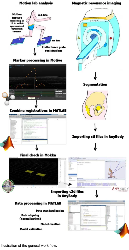
Measurements were done before the start of this thesis project. Raw data achieved in a motion laboratory had to be processed in advanced software tools. The first section considers briefly the recruitment of volunteers of the cross-sectional study. The other sections discuss the work flow from preprocessing to data normalization, modelling and validation. An impression of the data analysis work flow is shown in figure 12. Ethical approval for this study was obtained the Ghent University Hospital Ethics Committee (Corneel Heymanslaan 10, Ghent, Belgium) (approval number EC2014/0286).
2.1
Study sample
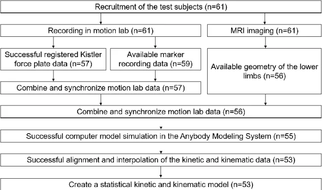
Sixty-one asymptomatic Caucasian healthy men participated to the study. These volunteers were aged between 17 and 28 years old. The admission requirement was practicing sports two or more hours a week. Subjects with overweight (body mass index (BMI) > 25) were excluded. As specified in figure 13, some subjects had an incomplete or incorrect registration.
Figure 13. Flow chart of the raw data processing. For some subjects, there was missing data.
No women were included into the data sample because similar studies were also based on male populations and the sample size is rather small to deal with potential gender differences. A description of the study population is shown in table 1.
Descriptive variable Mean (95% CI*) Normal values
Height (cm) 181.79 (180.08-183.51) Not applicable
Weight (kg) 71.75 (69.63-73.88) Not applicable
Body mass index (kg/m²) 21.70 (21.16-22.23) 18,5 – 25 (50) Sport activity (hours per week) 3.40 (2.76-4.03) Not applicable Center-edge angle (°) 28.41 (27.19-29.63) 25° – 39° (15, 32) Alpha angle (°) 64.61 (62.38-66.84) < 55° (15, 32) Centrum-collum-diaphyseal angle
or neck- shaft angle (°)
129.24 (127.99-130.49) 125° – 135° (32)
Femoral anteversion angle (°) 9.40 (7.30-11.49) < 15° (32) * confidence interval of the mean
The anthropometric measurements are defined in the introduction chapter.
Table 1. Demographic and anthropometric characteristics of the study population.
Upon signing the informed consent form, the participants were asked to perform specific movements like the right-forward kick lunge step (see also figure 2). In addition, the volunteers underwent full lower limbs MRI. In both examinations, twenty-eight reflective markers were stuck on the skin of each subject on palpable anatomical landmarks.
2.2
Motion lab analysis
Next to the markers on the body, nine reflective spheres were fixed to the left and right force plate. The applied force plates were developed by the Kistler Group (Winterthur, Switzerland). Three non-collinear points on the plates are each measured by three coordinates in order to define a plane. The force plate did not register only normal forces like a balance, but also friction forces in two dimensions. If a subject stands still, the sum of the left and right ground reaction forces will be equal to the body weight vector because there would be no forces in the plane of the plate surface.
After calibration setup, eight synchronized cameras recorded the optical markers at 15 Hz during subjects were doing a lunge. A marker point will be registered when it is detected by at least three cameras. A frequently occurring phenomenon in the recording is that of the temporarily invisibility. Motive will interpret a single twinkling marker as multiple different markers. Therefore, it is up to the experimenter to go over the entire recordings afterwards. Motive is the editing software tool that belongs to the Optitrack motion capture system (Natural Point Inc., Corvallis, Oregon, USA).
Finally, the markers should receive a label code in a systematic manner, so Anybody (cf. chapter 2.3) will be able to retrieve the path of the anatomical structures. Spatial marker trajectories are saved as C3D files. This public domain binary file format is the biomechanical data standard used by many commercial motion capture systems. Find out how to edit the captured markers in appendix 1.
In the next step, the C3D files were checked in Mokka (Motion Kinematic & Kinetic Analyzer, Biomechanical Toolkit (BTK)) for any mistakes in trajectories and labeling. Mokka is an open-source software application available on GitHub.
Registrations of the Kistler® force plates were saved as CSV (comma separated values) files while the test subjects performed the movements one after another. Arnaud Van Branteghem (Master of Science in Electromechanical Engineering, University of Ghent, Belgium) has written M-code to add the ground reaction forces to the C3D files in MATLAB (MATLAB 9.0 or release R2016a, MathWorks, Natick, Massachusetts, USA) (51).
2.3
Computer simulation in a musculoskeletal model
Simulations in musculoskeletal modeling software are crucial in this study, also for kinematic data, because patient specific bone geometry and marker positions can be incorporated here. It will enable us to calculate angles at 0,01° precision. Many musculoskeletal models in literature do not focus on this patient-specific variability as they use scaled generic models (52, 53).
The obtained C3D files from section 2.2 were imported into the AMS (version 7.1.0, Anybody Technology, Aalborg, Denmark). The STL files containing the subject-specific geometry of the hip, tibia and fibula, were imported to ensure the bone morphology in the motion capture (MoCap) musculoskeletal models. These STL files were created by doing segmentation of MRI images made by a 3-Tesla MAGNETOM Trio-Tim System (Siemens AG, Erlangen, Germany) in the University Hospital of Ghent. Other morphologic input like muscle position and muscle thickness was obtained from the Twente Lower Extremity Model 2.0 (TLEM 2.0) dataset (17). Marker point trajectories are the motion input of the kinematic and subsequent inverse dynamics analyses in Anybody for the MoCap musculoskeletal model. Marker positions are liable to skin shift because the markers are placed at some distance from the bony landmarks. This skin artifact is thought to be one of the main causes of noise and errors in the output data. Therefore, the AMS exploits so-called soft drivers, as described in appendix 2 (54). A motion capture filter with a cutoff frequency of 2 Hz was used for this purpose. Another reason why errors could occur is the mathematical optimization problem concerning the muscle recruitment solver in the AMS. This solver estimates the load distribution over muscle groups that is
different for every human. The muscles strengths and tendons lengths are not subject-specific and are likely to vary from the cadaveric dataset, especially in the simulation of young men in a good state.
2.4
Creating a statistical model
The generated kinematic and kinetic data in the AMS was labeled in vectors in MATLAB. As common with most of the researchers in this topic, forces and moments were standardized for body weight (BW) and BW x height.
refers to gravitational acceleration and is defined as or .
The units of the forces and moments are respectively (Newton) and (Newton meter). The latter should not be confused with (joule).
The beginning and the end frames of entire recorded lunges are rather useless due to irrelevant transients, so the data should be trimmed. To the author’s knowledge, the variance can be summarized best by only using data from the closed chain part of the movement. Analogously, the time frame with the most bended state will vary from the center of the recorded data. Here, the center of the lunge data is defined as the frame with the highest right knee flexion. After data trimming and aligning, the final step in the data summarization was an interpolation of the kinematic values from the MoCap musculoskeletal model output in order to get data for instances from 0 to 100% progress of the lunge. Here, 0% proceedings will refer to the first frame where the right foot was on the right force plate, 50% proceedings to the peak knee flexion and 100% proceedings to the last frame with the right foot on the right force plate. For this purpose, the applied method was Piecewise Cubic Hermite Interpolating Polynomial (PCHIP) interpolation.
In contrast to some gait studies, only kinematic data was included in the model (38, 55). Kinetic data was left aside because it is generated by using the kinematic data in Anybody in an inverse dynamics analysis. Furthermore, a mode cannot describe angles as well as forces, what is like comparing apples and oranges. On top of that, only data from the right leg is used based on the idea that this leg is loaded more than the left one during lunge motion.
Note that those three hip parameters are also known as the hip Euler angles. More about the hip Euler angles and the anterior pelvis tilt (APT) is written in Appendix 2.
All the subject vectors were combined in a training matrix , such that each column represents a test subject or variable.
represents the number of the test subjects. serves as the diagonal matrix with the row-wise standard deviations of .
with
After model normalization by row-wise standard deviation and mean centering, a residual matrix is created.
with and
In , the variance of each row is equal to because of the normalization. A model of the variance was created based on principal component analysis. Principal component analysis (PCA) is a powerful dimensionality reduction technique developed by Karl Pearson. It is not a method to investigate the center size of the data but the common variability. PCA is mathematically defined as an orthogonal linear transformation. In other words, the dimensions (called “principal components” or “modes”) are not correlated with each other. PCA transforms the data, as such most of the variance of the data will be in the first components. This enables to investigate how the variance of a kinematic parameter will affect another, and that is just what the modelling does: capturing the common variance in modes (38, 56). There is an ability to generate population data from a small set of clinical data. Altogether, PCA is a reliable tool capturing salient features of the original kinematic (and kinetic) waveforms (57). More details about the PCA principles are in appendix 3.
2.5
Model validation
Validation with real data was not possible because there were no kick lunges found in the open source Orthoload database.
Four model validation analyses based on (subsets of) the training dataset are investigated in MATLAB. ‘Goodness’ measures are chosen according to the statistical shape modeling study of Styner et al. in which there is also a PCA dimensionality reduction algorithm (58, 59). This study is the first to provide such an approach, implemented for a kinematic model.
2.5.1 Model accuracy
The first validation test analyzes how much percentage of variance seems enough to reconstruct the data. A model consist of some PCs describing a certain amount of variance. Here, the root-mean-square error (RMSE) is computed as the average absolute difference between original training data and reconstructed data for models with 90%, 95% and 98% variance of the original data.
2.5.2 Model compactness
The model will be compact enough, if it can describe the variance in kinematic observations with a minimal number of modes. The compactness for the first m principal components equals to the cumulative variance of that modes for all kinematic parameters included in the model
, relative to all variance of the training data .
2.5.3 Model generalization
The model generalization quantifies the ability of kinematic models to represent new kinematic instances. The generalization ability is evaluated by performing a series leave-one-out tests on the training data. The question here is: how many training samples are necessary to approach the population precisely? If having enough training samples, we expect the model to be able of describing unseen data quite accurately (60). The generalization value can be interpreted as the median out-of-sample accuracy value.
The generalization evolution gives the RMSE between excluded subject data and the best matched 95% variance model ’ values of randomly selected training data, by ascending number of training samples in the model ’. The higher the test value, the higher the precision of the median generalization value. Here, the number of models created for each number of training samples amounts to .
2.5.4 Model specificity
A population model can generate new data. The model specificity measures the soundness of new instances randomly generated by the developed model . Models with 90%, 95% and 98% of variance are tested. refers to a randomly generated subject.
We assume that the PCs of the model are normally distributed (38, 56). For each observation , an imaginary subject is defined by choosing random normal distributed values
for each mode in the model with :
The RMSE is defined as the error between the virtually subject data and the most similar sample in the training data set. The specificity value can be interpreted as the median approximation error of generated subjects. The higher the test value, the higher the precision of the specificity. Here, the number of models created is set to .
3 Results
3.1
The kinematic model of the lower limbs during lunge
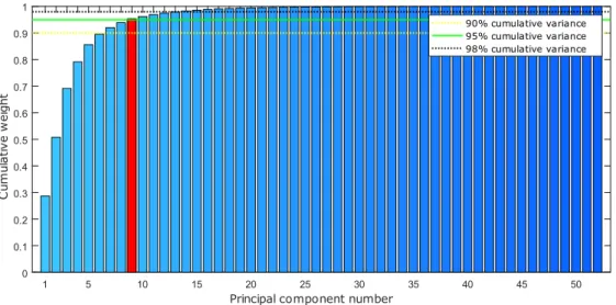
Figure 14. Scree plot with the cumulative variance of the modes (or PCs) capturing the training data.
Models with 90%, 95% and 98% variance can be obtained.
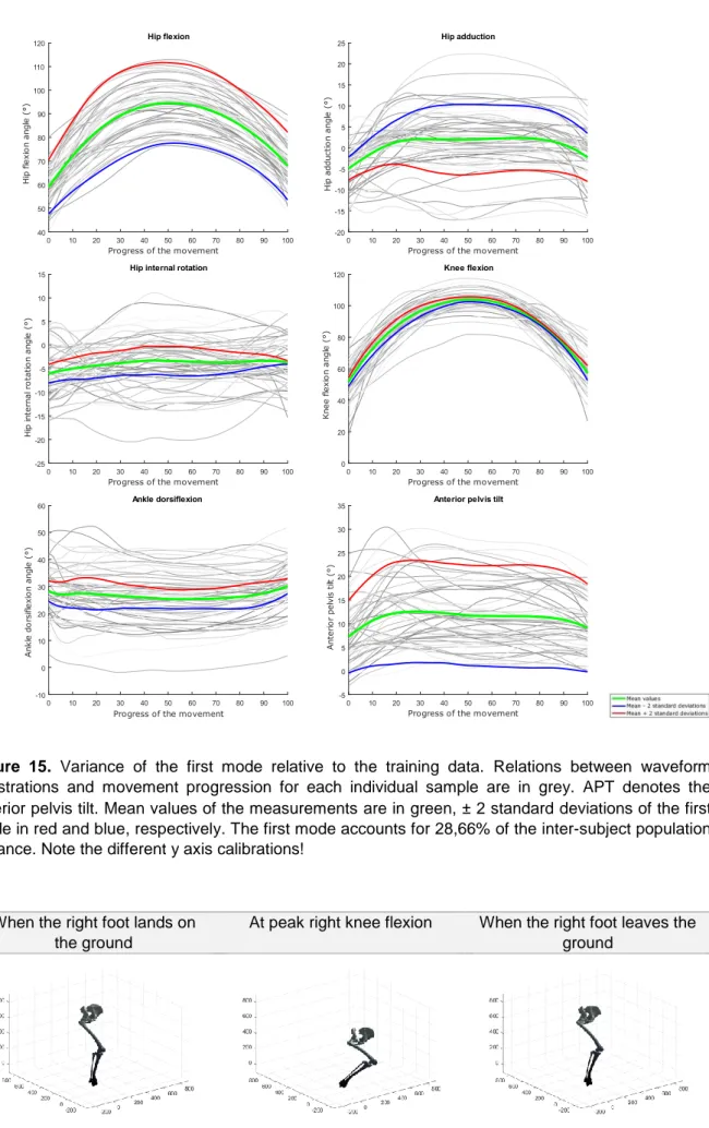
Waveform data from the Euler angles of the hip joint, pelvis tilt, knee and ankle flexion are represented by grey curves in figures 15, 17 and 19. The average peak flexion is 94,76° for the hip joint and 104,18° for the knee joint. For squat trials, this is 107° and 112°, respectively (61). The average peak ankle dorsiflexion amounts to 32,15°, 3,87° for the average peak hip adduction and 0.30° for the average peak hip external rotation. The averaged ROM of the pelvis tilt amounts to 8,53° (during the closed chain part of motion). Variances of the modes 1 to 3 are illustrated in figures 15 to 20, respectively. Figure 14 displays the cumulative variance of all modes from the PCA. The first three modes are representative of 69,14% of the population variance. From the fifth mode on, the PCs contain less than 10% of variance.
. . . . . . . . .
Figure 15. Variance of the first mode relative to the training data. Relations between waveform
registrations and movement progression for each individual sample are in grey. APT denotes the anterior pelvis tilt. Mean values of the measurements are in green, ± 2 standard deviations of the first mode in red and blue, respectively. The first mode accounts for 28,66% of the inter-subject population variance. Note the different y axis calibrations!
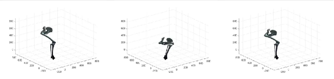
When the right foot lands on the ground
At peak right knee flexion When the right foot leaves the ground
Figure 16. Graphical representation of the variance described by the first principal component.
Figure 17. Variance of the second mode relative to the training data. Mean values of the measurements
in green ± 2 standard deviations of the second mode in red and blue. The second mode accounts for 22,11% of the inter-subject population variance.
Figure 18. Graphical representation of the variance described by the second principal component.
When the right foot lands on the ground
At peak right knee flexion When the right foot leaves the ground
Figure 19. Variance of the third mode relative to the training data. Mean values of the measurements
in green ± 2 standard deviations of the third mode in red and blue. The third mode accounts for 18,37% of the inter-subject population variance.
Figure 20. Graphical representation of the variance described by the third principal component.
3.2
Validation results
In table 2, the within-model accuracy and specificity are given for each set of observations. The model accuracy for 9 modes (95,27% of variance) ranges from 0,11 to 0,16 degrees. The model specificity for this model varies from 0,91 to 6,19 degrees. All values were higher than the 0,01° resolution threshold of the musculoskeletal model.
When the right foot lands on the ground
At peak right knee flexion When the right foot leaves the ground
Set of kinematic parameters Model accuracy Model specificity* Median ° RMSE (° IQR**) Median ° RMSE (° IQR**) % of inter-individual variance in the population 90% 95% 98% 90% 95% 98% Hip flexion-extension 0,22 (0,12) 0,15 (0,08) 0,10 (0,05) 6,19 (1,16) 6,19 (1,16) 6,19 (1,17) Hip adduction-abduction 0,14 (0,07) 0,12 (0,07) 0,08 (0,05) 1,48 (0,87) 1,48 (0,87) 1,49 (0,87) Hip rotation 0,12 (0,09) 0,11 (0,06) 0,05 (0,03) 1,69 (0,61) 1,69 (0,61) 1,70 (0,62) Knee flexion-extension 0,18 (0,18) 0,13 (0,08) 0,10 (0,06) 5,53 (0,78) 5,54 (0,78) 5,54 (0,78) Ankle flexion-extension 0,17 (0,10) 0,16 (0,11) 0,11 (0,06) 2,19 (1,27) 2,19 (1,27) 2,20 (1,27) Pelvis tilt 0,17 (0,10) 0,13 (0,08) 0,07 (0,05) 0,90 (0,67) 0,91 (0,66) 0,90 (0,66) All data 0,16 (0,10) 0,13 (0,08) 0,09 (0,06) 2,05 (4,02) 2,05 (4,02) 2,05 (4,01)
* model specificity by using random sampled test data ** IQR = interquartile range
Table 2. Validation analysis of the kinematic model.
The boxplots in figure 21 illustrate the in-sample model accuracy for ascending number of included components. The RMSE are taken from the original training data relative to reconstructed data with the model. Figure 14 shows the compactness of the training data after dimensionality reduction through PCA.
Figure 21. RMSE for the original training data versus the reconstructed data from models with an
increasing number of PCs.
Regarding figure 22, for each training data amount going from 4 to 52, 10.000 models including 95% population variance are created to reconstruct an excluded subject resulting in an error between the original and the reconstructed data. These out-of-sample accuracy RMSE are given on the y axis in boxplots. The median out-of-sample RMSE is in blue. There is also plotted a green horizontal curve of the in-sample model accuracy of the 95% model from
. . . . . . . . . . . . . . . . . . . . . . . . . . . . . . . . . . . . . . . . . . . . . . . . . . . . . . . . . . . .
section 3.1. The out-of-sample accuracy is clearly stagnating for the hip flexion (around 1,52° RMSE starting from 40 training samples), hip abduction (around 1,21° RMSE starting from 20 samples), hip rotation (around 0,61° RMSE starting from 33 samples), knee flexion (around 1,17° RMSE starting from 50 samples) and pelvis tilt (around 0,86° starting from 42 samples). Only the ankle flexion generalization continues to decline a little by increasing number of training samples. Conversely, the difference with the in-sample accuracy is very small, notably 0,2099° for 53 training samples.
. . . . . . . . . . . . . . . . . . . . . . . . . . . . . . . . .
Figure 22. Accuracy evolution of waveform data for different levels of prior knowledge expressed as
amounts of training data in a kinematic model and the in-sample target accuracy (green horizontal line). Boxplots reproduce the RMSE of the reconstructed data with 95% variance versus the original training data. In order to facilitate interpretation, the axes are linear scaled on the left side, whereas on the right, they are both log-scaled.
. . . . . . . . . . . . . . . . . . . . . . . . . . . . . . . . .