Application of principal component analysis to time series of daily air pollution and mortality

(1)

Application of principal component analysis to time series of daily air pollution and mortality CM Quant, PH Fischer, E Buringh, CB Ameling, DJM Houthuijs, FR Cassee

This investigation has been performed by order and for the account of NOVEM, within the framework of project 650010, Healths effects of particulate matter.

(2)

(3)

Abstract

The overall objective of this study was to investigate whether cause-specific daily mortality (i.e. respiratory, cardiovascular, pneumonia, COPD and total mortality) can be attributed to specific sources of air pollution.

Therefore we formulated the following aims:

1. To apply a principal component analysis (PCA) on air pollution data in order to provide a meaningful description in components that are interpretable in terms of different sources of air pollution.

2. To quantify the association between daily mortality (total, cardiovascular diseases, respiratory, pneumonia and COPD mortality) and the source-specific components. 3. To investigate the effect of season-specific associations between daily mortality and the

components.

4. To consider whether this method leads to new insights with regard to the approach of mortality analyses.

The first part of this report is focussed on the principal component analysis and the allocation of new variables into source-related variables.

The second part relates to the quantification of associations between mortality and the principal components (source-related explanatory variables).

Based on data series used for the mortality analyses in Fischer et al. (in preparation), (concerning daily mortality, air pollution and confounding variables in the period 1993-1998), we applied a principal component analysis on standardised air pollution data. We considered the first part of these principal components, that is the principal components with the largest variances, since these components are supposed to contain the most information and therefore can be used as summary of the air pollution data. We standardised the principal components and applied a varimax rotation on the loadings of the first part of the

standardised components (in our case on the first three, four and five components), to consider whether we obtain vectors that seem to reflect the pollution of specific source categories. We eventually used five principal components that explain 92% of the variance in the data. For these rotated components we computed the daily values and the corresponding lags, which were then used in the mortality analysis in Part two.

We identified five major components that can be related to source categories using principal component analysis: traffic, secondary inorganic transformations, bio-industry, industry and photochemical transformations.

These five components were analysed in relation to (cause-specific) mortality.

The association between these components and mortality was modelled with a generalised additive model (GAM), in one- and multi-component models. In these models also a large number of confounding variables were included, to correct for meteorological influences, influenza epidemics, time of the year etc.

(4)

Our conclusions of the study are:

1. Routinely collected air quality data can be used to identify at least five major components that can be related to source categories using principal component analysis: traffic, secondary inorganic transformations, bio-industry, industry and photochemical transformations.

2. Although PCA leads to a clear insight in the most important sources of the air pollution mixture in the Netherlands, the results do not exclude certain source categories from the policy process.

3. We found statistically significant associations between the components and daily mortality, both in one-component and in multi-component models. These associations were spread over the different rotated components; we did not find an indication for a sole causal factor for the observed mortality associations.

4. The strongest associations were found with the week-averages of the industrial component (significant for all mortality categories) and with the photochemical

component (significant for total, respiratory, pneumonia and COPD mortality). Also for the traffic-related, secondary inorganic transformations and the bio-industry components we found significant results, but with lower relative risks.

5. Comparing associations between different causes of death, relative risks were generally higher for pneumonia and respiratory mortality than for total mortality.

6. In the summer season, components generally had a higher impact on mortality than in the winter.

(5)

Samenvatting

Meer dan 100 epidemiologische studies, verspreid over de hele wereld, hebben een relatie aangetoond tussen dagelijkse variaties in de niveaus van luchtverontreiniging en dagelijkse sterfte. Ook in Nederland is deze relatie aangetoond. Omdat in de buitenlucht meerdere stoffen tegelijkertijd voorkomen, is het moeilijk om exact aan te geven welk onderdeel van het luchtverontreinigingsmengsel verantwoordelijk is voor de gevonden verbanden. Voor beleidsmakers is inzicht in de rol van de afzonderlijke componenten echter van groot belang, omdat kennis over de relevante componenten, en dus ook relevante bronnen, een effectief beleid ter vermindering van de gezondheidseffecten mogelijk maakt. In deze studie is gepoogd om door middel van een specifieke statistische methodiek de relatie tussen dagelijkse sterfte en vijf belangrijke bronnen van luchtverontreiniging te onderzoeken. De vraagstelling van het onderzoek was om een relatie te leggen tussen dagelijkse oorzaak-specifieke sterfte in de Nederlandse bevolking en oorzaak-specifieke bronnen van grootschalige luchtverontreiniging.

De volgende doelstellingen werden hierbij gehanteerd:

1. toepassing van principale componenten analyse (PCA) op luchtverontreinigingsgegevens, en om op basis van de resultaten van deze analyses verschillende bronnen van

luchtverontreiniging te kunnen identificeren.

2. de relatie tussen dagelijkse sterfte (totale, cardiovasculaire, respiratoire, longontsteking en COPD) en de bronnen te kwantificeren.

3. seizoensspecifieke relaties tussen sterfte en bronnen te onderzoeken.

4. aangeven in hoeverre deze methode nieuw inzicht geeft in de relatie luchtverontreiniging en sterfte.

Het eerste gedeelte van dit rapport beschrijft de methodiek van principale componenten analyse; het tweede deel beschrijft de relatie tussen sterfte en de geïdentificeerde bronnen. Op basis van bestaande datareeksen over de periode 1993-1998 van dagelijkse

sterftestatistieken en dagelijkse luchtverontreingingsniveaus, is een principale componenten analyse uitgevoerd op de luchtverontreinigingsdata. Resultaat van deze analyse was vijf principale componenten waarmee 92% van de variantie in de luchtverontreinigingsdata kon worden verklaard. Deze vijf componenten zijn vervolgens geanalyseerd in relatie tot de dagelijkse sterfte.

De geïdentificeerde componenten konden aan de volgende bronnen gerelateerd worden: verkeer, secundair anorganisch aërosol, bio-industrie, industrie en fotochemische verontreiniging.

Met behulp van “Generalised Additive Models” (GAM) is vervolgens de relatie onderzocht met sterfte, waarbij voor een groot aantal potentiële verstorende variabelen is gecorrigeerd. De conclusies van de studie zijn:

1. Op basis van principale componenten analyse van routinematig verzamelde gegevens over dagelijkse luchtverontreinigingsniveaus zijn vijf principale componenten te

identificeren die aan bronnen gerelateerd kunnen worden: verkeer, secundair anorganisch aërosol, bio-industrie, industrie en fotochemische verontreiniging.

(8)

2. Alhoewel met principale componenten analyse meer inzicht wordt verkregen in de rol van de afzonderlijke bronnen in het gehele mengsel van luchtverontreiniging, heeft dit inzicht er niet toe geleid dat bepaalde broncategorieën uitgesloten kunnen worden met betrekking tot de invloed op sterfte.

3. Er zijn statistisch significante associaties tussen de componenten en dagelijkse (oorzaakspecifieke) sterfte aangetoond; deze associaties zijn gevonden met alle vijf componenten, waarbij er geen voorkeur werd gevonden voor een specifieke factor. 4. De sterkste associaties werden gevonden voor de industriële component en voor de

fotochemische componenten. Voor de andere componenten werden eveneens significante associaties gevonden, maar met een lager relatief risico.

5. Relatieve risico’s voor de specifieke doodsoorzaken longontsteking en respiratoire sterfte waren in het algemeen hoger dan voor de totale dagelijkse sterfte.

6. Voor het zomerseizoen werden in het algemeen hogere relatieve risico’s gevonden dan voor het winterseizoen.

(9)

1 Introduction

A large number of epidemiological studies, conducted all over the world, have reported on associations between acute health effects and exposure of populations to particulate matter (PM), especially on PM10 (Samet, 2002). Most of the studies focused on the association

between mortality or hospital admissions and particulate matter. Reported health outcomes are pulmonary function decrements, respiratory symptoms, hospital and emergency department admissions and mortality. More recently, studies were published that focused on birth defects and general practitioner visits in relation to PM exposure (Wilhelm et al., 2003; Hajat et al., 2002).

Recently, in the Netherlands a study was performed on the association between mortality and air pollution over the period 1986-1994 (Hoek et al., 1997, 2000). The results of this study showed statistically significant associations between several air pollution components (including PM10) and daily mortality. The relative risk (RR) of that study was 1.02, 95%

confidence interval (1.003, 1.034), for a change of the PM10 concentration with 100 µg/m3,

resulting in approximately 1000 premature deaths per year in the Netherlands attributable to PM10. In 2001 an extension of the time series analyses on mortality and air pollution was

conducted, considering the period 1992-1998, see Fischer et al. (in preparation). In comparison to earlier analyses on this relationship, a larger PM10 data set (4-5 additional

years, resulting in a seven - eight year time series) was analysed in single- and two-pollutant models. The results of this study were along the same lines as the previous study with a RR of 1.04 and 95% confidence interval (1.025, 1.047) for a change of the PM10 concentration

with 100 µg/m3_.

A complicating factor in studying associations between air pollution and mortality is that air pollution concentrations are generally mutually positively correlated, since e.g. meteorology has the same influence on all concentrations. High correlations between components also occur when pollutants have a common source, for example traffic or industry. Fitting several highly correlated air pollution components in the same model leads to inflation of standard errors and does not lead to meaningful results. Therefore in multi-component models, one usually fits only those air pollution components that have a low interrelation.

Although there is consensus in the scientific literature about the consistency of the associations found in epidemiological time-series studies, it is still unknown what the responsible causal factors for these associations can be. Therefore both toxicological and epidemiological research is focusing on the sources of air pollution that may explain the association between PM and health effects. One of the first studies in this context has been presented by Dr. Halûk Özkaynak at the “PM2000: Particulate Matter and Health” conference (Özkaynak et al., 2000). He presented the application of principal component analysis techniques on a set of air pollution and meteorological data to identify sources. Subsequently, these principal components (among other things auto, fossil fuel, ozone/regional haze, etc.) were used in time-series models to estimate the association between cause-specific mortality and each of these components. Analysis of an extensive twenty years of mortality and pollution records for the greater Toronto area showed statistically significant associations between PM, O3 and motor vehicle related air pollution,

and the various cause specific daily mortality categories. Specifically, the average contribution of auto-related pollution in Toronto to either daily total or cardiovascular

(10)

mortality was estimated to be around 2%, while the average contribution of motor vehicle pollutants to acute respiratory or pneumonia deaths was predicted to be about 5%. Several recent studies reported source-oriented evaluation of PM associated health effects using factor and principal component analysis to estimate daily concentrations due to underlying source types (e.g. mobile emissions, soil, coal) (Laden et al., 2000; Mar et al., 2000; Tsai et al., 2000). In summary, these studies suggest that a number of source-types are associated with mortality, including automobile emissions, coal burning, and vegetative burning.

Laden (2000) used the elemental composition of size-fractioned integrated 24-hr fine particle measurements, collected at least every other day from 1979 until the late 1980s, to identify several distinct source-related fractions. They examined the association of these fractions with daily mortality in six cities. In the fine fraction, 15 elements were routinely found: silicon, sulphur, chlorine, potassium, calcium, vanadium, manganese, aluminium, nickel, zinc, selenium, lead, copper and iron. With specific rotation factors per city up to 5 common factors from the 15 specified elements were identified. The factors identified in all six cities were a silicon factor (classified as soil and crustal material), a lead factor (classified as motor vehicle exhaust), and a selenium factor (classified as coal combustion sources). Dependent on the cities, additional factors identified were vanadium (fuel oil combustion), chlorine (salt), and selected metals (nickel, zinc or manganese) as possible targets and sources. For each city the daily mortality was regressed on the daily score for each of the identified factors. For the three source factors identified in all metropolitan areas, the strongest increase in daily mortality was associated with the mobile sources factor (lead). The coal factor (selenium) was also positively associated with mortality with the exception of one city (Topeka). The crustal factor in fine particulate matter was not associated with mortality. There were some suggestions that the fuel oil combustion factor was positively associated with mortality, but this association was non-significant. In models with measurements for the individual elements, nickel, lead and sulphur were significantly associated with mortality. These results indicate that combustion particles in the fine fraction from mobile and coal combustion sources, but not fine crustal particles, are associated with increased mortality.

Mar et al. (2000) conducted a principal component analysis and varimax rotation on the daily concentrations of the chemical components of PM2.5 and on the gaseous species emitted by

combustion sources (CO, NO2, SO2) in Phoenix over the period 1995 – 1997 to assess the

association with total and cardiovascular mortality. Chemical components were Al, Si, S, Ca, Fe, Zn, Mn, Pb, Br, K, Organic Carbon (OC) and Elemental Carbon (EC). Results from the analyses with five factors were presented. Identified factors were: motor vehicle exhaust and resuspended road dust (high loadings (or correlations) on Mn, Fe, Zn, Pb, EC, CO and NO2),

soil (high loadings on Al, Si, Fe), vegetative burning (high loadings on OC and “soil corrected” K), a local source of SO2 (high loading on SO2) and regional sulphate (a high

loading on S). Total mortality was not associated with the identified factors, except the regional sulphate with a lag of 0 days. Cardiovascular mortality was significantly associated with the factors representing motor vehicles and vegetative burning. The results based on the factors were consistent with time-series results for individual pollutants (CO, NO2, K, EC,

OC).

Tsai et al. (2000) also applied factor analysis and poisson regression to a data set with mortality and extensive PM chemical specification measurements (including trace metals, sulphate and particulate organic matter). Ambient pollution data were collected between 1981 and 1983 at three sites in New Jersey: Newark, Elizabeth and Camden. Chemical components included in the factor analysis with varimax rotation were Pb, Mn, Cd, V, Zn, Fe, Ni, SO4and

(11)

CO. Tracers that were used to identify PM sources were: Mn and Fe for dust, SO4 for

secondary aerosol, Zn, Cd and Cu for various industrial sources. Up to 7 sources were identified in the factor analyses:

Source High loading

Oil burning V and Ni Industrial-1 Cu Geological Mn Industrial-2 Zn Motor vehicle CO Sulphate SO4 Industrial-3 Cd

In Newark oil burning (tracers: V and Ni), industrial sources (tracer: Zn and Cd) and sulphate aerosol showed positive relationships with total daily mortality. For cardiopulmonary deaths only sulphate was a significant factor. In Camden results indicated that oil-burning and motor vehicle emissions (tracers: Pb and CO) were two important sources for total daily mortality; sources traced by copper showed a negative association with total daily deaths. Three PM sources were significant predictors for cardiovascular mortality: oil burning, motor vehicles and sulphate. In Elizabeth total daily mortality showed a negative association with resuspended dust (tracers: Fe and Mn). Three factors were significantly associated with cardiopulmonary mortality: industrial sources (tracer: Cd) showed positive associations and resuspended dust and industrial sources traced by copper showed negative associations. In the Netherlands, the National Institute for Public Health and the Environment operates the ambient air quality monitoring network. Large time series are available of daily concentrations of various pollutants. It would be useful to create source-related variables from these time series, like in the above described literature, which can be used to model the association between sources of air pollution and mortality. This can be interesting for policy makers, since this might give a clue which sources are most important in this relationship. This study will focus on the feasibility of a principal component analysis on air pollution data for the Netherlands.

The overall objective of this study is to investigate whether cause-specific mortality (i.e. respiratory, cardiovascular, pneumonia, COPD and total mortality) can be attributed to specific sources of air pollution.

Therefore we formulated the following aims:

1. To apply a principal component analysis on air pollution data in order to provide a meaningful description in components that are interpretable in terms of different sources of air pollution.

2. To quantify the association between mortality (total, cardiovascular diseases, respiratory, pneumonia and COPD mortality) and the source-specific components.

3. To investigate the effect of season-specific associations between mortality and the components.

4. To consider whether this method leads to new insights with regard to the approach of mortality analyses.

(12)

The first part of this report is focussed on the principal component analysis and the allocation of new variables into source-related variables.

The second part relates to the quantification of associations between mortality and the principal components (source-related explanatory variables). Finally, we will discuss the results in relation with previous findings and related studies.

(13)

2 Part one: Principal component analysis on air

pollution data

2.1 Overview

We will shortly describe the principal component analysis; the results of the principal component analysis together with a more detailed explanation will follow later.

Based on data series used for the mortality analyses in Fischer et al. (in preparation), (concerning daily mortality, air pollution and confounding variables in the period 1993-1998), we apply a principal component analysis on standardised air pollution data. We consider the first part of these principal components, that is the principal components with the largest variances, since these components are supposed to contain the most information and therefore can be used as summary of the air pollution data. We standardise the principal components and apply a varimax rotation on the loadings of the first part of the standardised components (in our case on the first three, four and five components), to consider whether we obtain vectors that seem to reflect the pollution of specific source categories. We will eventually use five principal components that explain 92% of the variance in the data. For these rotated components we compute the daily values and the corresponding lags, which will be used in the mortality analysis in Part two. We list the consecutive steps for later reference: 1. PCA of the standardised air pollution concentrations.

2. Standardise the principal components.

3. Apply a varimax rotation on the first standardised components.

4. Determine the number of (rotated) principal components we want to use, such that the rotated components are interpretable in terms of sources of air pollution.

5. Compute the daily values of the rotated principal components.

2.2 Data

For a more detailed description of the data we refer to Fischer et al. (in preparation), in which the same data are used.

For the principal component analyses we use air quality data of the period 1993-1998, obtained from the National Institute for Public Health and the Environment (RIVM). The pollutants involved are PM10, black smoke (BS), carbon monoxide (CO), nitrogen oxide

(NO), nitrogen dioxide (NO2), ammonia (NH3), nitrate (NO3), sulphate (SO4), sulphur

dioxide (SO2) and ozone (O3). We use the daily averages of the concentrations (also averaged

over the Netherlands) of these pollutants, except for ozone, of which we use eight-hour averages (12.00 to 20.00 hours).

2.3 Statistical software

(14)

2.4 Results and explanation of the principal component

analysis

2.4.1 Principal component analysis

We first sketch the idea of a principal component analysis (PCA), as far as it applies to our specific context. For details on the subject we refer to Jolliffe, (1986). In the following, we will talk about the mean, the covariance etc. of certain air pollutant concentrations. This might be a bit misleading, of course these concentrations are not at all independent samples from a multivariate probability distribution, but are also influenced by e.g. meteorology, day of the week and time of the year. We use the mean, covariance etcetera of the daily concentrations in the period 1993 –1998.

We have a database of air pollution data, containing the daily concentrations of the pollutants PM10, BS, NH3, CO, NO, NO2, SO2, O3, NO3 and SO4 in the period 1993-1998. We shift these

concentrations such that the shifted concentrations have zero means, i.e. we subtract the means of the original concentrations. In a principal component analysis, a new co-ordinate system is chosen (the new co-ordinates are called principal components). Each principal component is a linear combination of the shifted (and eventually also standardised) concentrations, obeying certain conditions. For i∈

{

1,L10

}

, the _{i principal component is}th

written as: , 4 10 , 3 9 , 3 8 , 2 7 , 2 6 , 5 , 4 , 3 3 , 2 , 10 1 , SO a NO a O a SO a NO a NO a CO a NH a BS a PM a PC i i i i i i i i i i i + + + + + + + + + + =

the a_i_,_j,i,j∈

{

1,L,10

}

are real constants specified later. Here PM ,₁₀ BSetcetera are the (eventually standardised) shifted concentrations of PM10, BS etc. We writea for the vector_i

) , ,

(a_i_,₁ K a_i_,₁₀ . The constants a_i_,_j (which are called loadings) are chosen such that: • The length of the vectors a equals 1, i.e.i ai2,1 +L+ai2,10 =1.

• The first principal component PC1 is chosen such that Var(PC1) is maximal.

• Then the second principal component is chosen such that Var(PC₂) is maximal under the restriction that PC₁ and PC₂are uncorrelated.

• In general, the _{j principal component is chosen such that}th ₍ ₎ j PC

Var is maximal on the condition that PC and _k PC are uncorrelated for _j k∈

{

1,L, j−1

}

.

When we use shifted concentrations (and not standardised), this leads to the result that )

(PC₁

Var is equal to the largest eigenvalue of the covariance matrix of the concentrations and a₁a corresponding eigenvector of length one, Var(PC₂)is equal to the second largest eigenvalue and a₂a corresponding eigenvector of length one, etc. When we use standardised concentrations (i.e. shifted concentrations divided by the corresponding standard deviations) a similar correspondence holds, but now with the correlation matrix of the concentrations. As mentioned in Jolliffe (1986) section 2.3, a principal component analysis depends on the scale of the measurements (e.g. the loadings in the correlation and covariance case are not equal, nor can the first be directly obtained from the second). Therefore we should decide

(15)

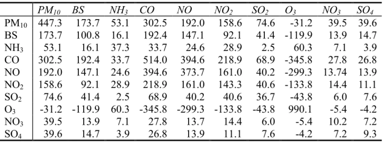
whether we want to rescale the measurements. When shifted concentrations (without dividing by the standard deviation) are used, the pollutants with the largest variance tend to dominate the first principal component(s). The covariance matrix of the air pollution concentrations in the period 1993-1998 is displayed in Table 1 and the correlations are given in Table 2 below.

Table 1 Covariances of the air pollution concentrations

PM10 BS NH3 CO NO NO2 SO2 O3 NO3 SO4

PM10 447.3 173.7 53.1 302.5 192.0 158.6 74.6 -31.2 39.5 39.6 BS 173.7 100.8 16.1 192.4 147.1 92.1 41.4 -119.9 13.9 14.7 NH3 53.1 16.1 37.3 33.7 24.6 28.9 2.5 60.3 7.1 3.9 CO 302.5 192.4 33.7 514.0 394.6 218.9 68.9 -345.8 27.8 26.8 NO 192.0 147.1 24.6 394.6 373.7 161.0 40.2 -299.3 13.74 13.9 NO2 158.6 92.1 28.9 218.9 161.0 143.3 40.6 -133.8 14.4 11.1 SO2 74.6 41.4 2.5 68.9 40.2 40.6 36.7 -43.8 6.0 7.6 O3 -31.2 -119.9 60.3 -345.8 -299.3 -133.8 -43.8 990.1 -5.4 -4.2 NO3 39.5 13.9 7.1 27.8 13.7 14.4 6.0 -5.4 10.2 7.2 SO4 39.6 14.7 3.9 26.8 13.9 11.1 7.6 -4.2 7.2 9.3

Table 2 Correlations of the air pollution concentrations

PM10 BS NH3 CO NO NO2 SO2 O3 NO3 SO4

PM10 1.00 0.82 0.41 0.63 0.47 0.63 0.58 -0.05 0.59 0.61 BS 0.82 1.00 0.26 0.85 0.76 0.77 0.68 -0.38 0.43 0.48 NH3 0.41 0.26 1.00 0.24 0.21 0.40 0.07 0.31 0.36 0.21 CO 0.63 0.85 0.24 1.00 0.90 0.81 0.50 -0.48 0.38 0.39 NO 0.47 0.76 0.21 0.90 1.00 0.70 0.34 -0.49 0.22 0.24 NO2 0.63 0.77 0.40 0.81 0.70 1.00 0.56 -0.36 0.38 0.31 SO2 0.58 0.68 0.07 0.50 0.34 0.56 1.00 -0.23 0.31 0.41 O3 -0.05 -0.38 0.31 -0.48 -0.49 -0.36 -0.23 1.00 -0.05 -0.04 NO3 0.59 0.43 0.36 0.38 0.22 0.38 0.31 -0.05 1.00 0.74 SO4 0.61 0.48 0.21 0.39 0.24 0.31 0.41 -0.04 0.74 1.00

We see that the variances (on the diagonal of Table 1) of the air pollution concentrations are very different. Applying a principal component analysis to the shifted data leads to a result in which the loadings for the pollutants NO3, SO4, NH3 and SO2 are very small loadings in the

first components. We therefore decided to standardise the concentrations before applying a principal component analysis.

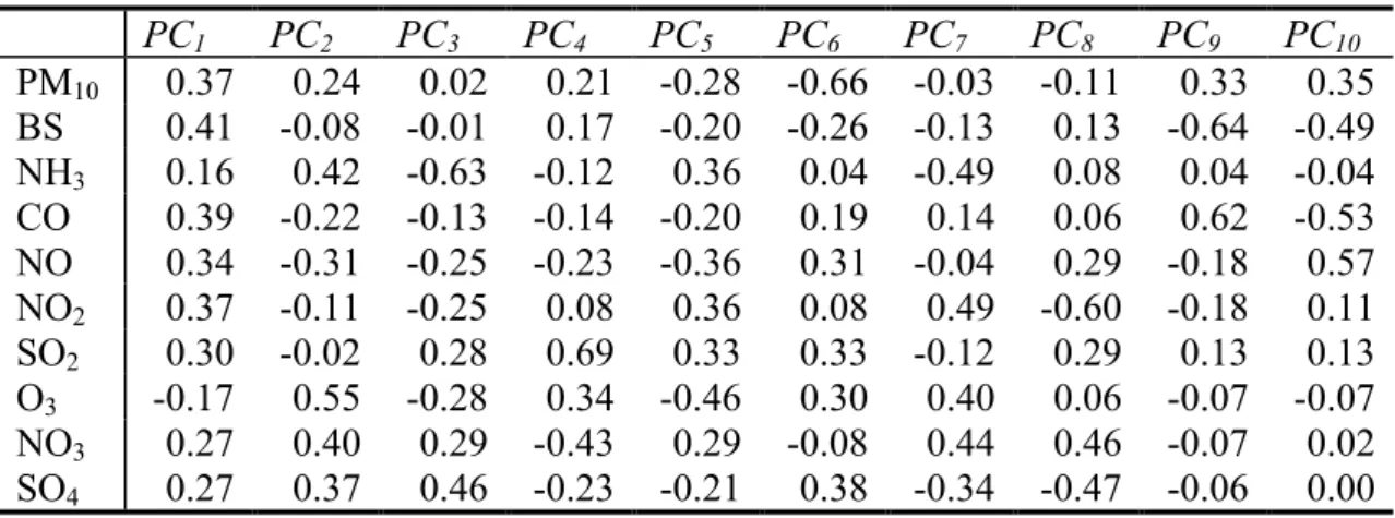
In Table 3 below, we see the loadings of the principal component analysis of the standardised air pollution concentrations, for example:

. 27 . 0 27 . 0 17 . 0 30 . 0 37 . 0 34 . 0 39 . 0 16 . 0 41 . 0 37 . 0 4 3 3 2 2 3 10 1 SO NO O SO NO NO CO NH BS PM PC + + − + + + + + + + =

Since the matrix of the numbers in Table 3 is orthogonal, we can also read this table from left to right, for example for the standardised concentration of PM10 we have:

(16)

. 35 . 0 33 . 0 11 . 0 03 . 0 66 . 0 28 . 0 21 . 0 02 . 0 24 . 0 37 . 0 10 9 8 7 6 5 4 3 2 1 10 PC PC PC PC PC PC PC PC PC PC PM + + − + − − − + + + =

Table 3 PCA of the standardised air pollution concentrations

PC1 PC2 PC3 PC4 PC5 PC6 PC7 PC8 PC9 PC10 PM10 0.37 0.24 0.02 0.21 -0.28 -0.66 -0.03 -0.11 0.33 0.35 BS 0.41 -0.08 -0.01 0.17 -0.20 -0.26 -0.13 0.13 -0.64 -0.49 NH3 0.16 0.42 -0.63 -0.12 0.36 0.04 -0.49 0.08 0.04 -0.04 CO 0.39 -0.22 -0.13 -0.14 -0.20 0.19 0.14 0.06 0.62 -0.53 NO 0.34 -0.31 -0.25 -0.23 -0.36 0.31 -0.04 0.29 -0.18 0.57 NO2 0.37 -0.11 -0.25 0.08 0.36 0.08 0.49 -0.60 -0.18 0.11 SO2 0.30 -0.02 0.28 0.69 0.33 0.33 -0.12 0.29 0.13 0.13 O3 -0.17 0.55 -0.28 0.34 -0.46 0.30 0.40 0.06 -0.07 -0.07 NO3 0.27 0.40 0.29 -0.43 0.29 -0.08 0.44 0.46 -0.07 0.02 SO4 0.27 0.37 0.46 -0.23 -0.21 0.38 -0.34 -0.47 -0.06 0.00

The variances and standard deviations of these principal components are displayed in Table 4.

Table 4 Variances and standard deviations of the principal components of the standardised concentrations

PC1 PC2 PC3 PC4 PC5 PC6 PC7 PC8 PC9 PC10

Var. 5.22 1.75 1.07 0.74 0.41 0.26 0.23 0.19 0.07 0.06 St. dev. 2.28 1.32 1.03 0.86 0.64 0.51 0.48 0.43 0.27 0.24

The idea is that, since the last principal components have very small variances, they contain less information than the first principal components with larger variances.

We standardise the principal components; i.e. we divide each principal component by its standard deviation. We denote the standardised principal components by *

j PC , where ) ( . * j j j PC dev st PC

PC = . When we standardise the components, also the loadings change. We get two new tables of loadings, depending on whether we want to express the standardised principal components as a linear combination of the standardised concentrations or the other way around. The results can be found in Table 5 and Table 6.

(17)

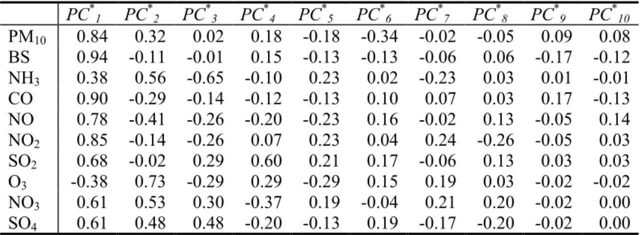
Table 5 Correlation loadings (of the standardised concentrations as linear combination of the standardised principal components)

PC*1 PC*2 PC*3 PC*4 PC*5 PC*6 PC*7 PC*8 PC*9 PC*10 PM10 0.84 0.32 0.02 0.18 -0.18 -0.34 -0.02 -0.05 0.09 0.08 BS 0.94 -0.11 -0.01 0.15 -0.13 -0.13 -0.06 0.06 -0.17 -0.12 NH3 0.38 0.56 -0.65 -0.10 0.23 0.02 -0.23 0.03 0.01 -0.01 CO 0.90 -0.29 -0.14 -0.12 -0.13 0.10 0.07 0.03 0.17 -0.13 NO 0.78 -0.41 -0.26 -0.20 -0.23 0.16 -0.02 0.13 -0.05 0.14 NO2 0.85 -0.14 -0.26 0.07 0.23 0.04 0.24 -0.26 -0.05 0.03 SO2 0.68 -0.02 0.29 0.60 0.21 0.17 -0.06 0.13 0.03 0.03 O3 -0.38 0.73 -0.29 0.29 -0.29 0.15 0.19 0.03 -0.02 -0.02 NO3 0.61 0.53 0.30 -0.37 0.19 -0.04 0.21 0.20 -0.02 0.00 SO4 0.61 0.48 0.48 -0.20 -0.13 0.19 -0.17 -0.20 -0.02 0.00

Table 6 Loadings of the standardised components as linear combination of the standardised concentrations PC* 1 PC*2 PC*3 PC*4 PC*5 PC*6 PC*7 PC*8 PC*9 PC*10 PM10 0.16 0.18 0.02 0.24 -0.44 -1.30 -0.07 -0.26 1.23 1.46 BS 0.18 -0.06 -0.01 0.20 -0.32 -0.51 -0.27 0.31 -2.36 -2.05 NH3 0.07 0.32 -0.61 -0.14 0.56 0.08 -1.02 0.18 0.16 -0.18 CO 0.17 -0.16 -0.13 -0.16 -0.30 0.38 0.28 0.14 2.28 -2.22 NO 0.15 -0.24 -0.24 -0.27 -0.57 0.61 -0.07 0.66 -0.66 2.38 NO2 0.16 -0.08 -0.25 0.10 0.56 0.15 1.02 -1.38 -0.65 0.46 SO2 0.13 -0.01 0.27 0.81 0.51 0.65 -0.25 0.68 0.46 0.54 O3 -0.07 0.42 -0.27 0.39 -0.71 0.59 0.83 0.14 -0.27 -0.28 NO3 0.12 0.30 0.28 -0.50 0.46 -0.15 0.91 1.05 -0.26 0.08 SO4 0.12 0.28 0.45 -0.26 -0.33 0.75 -0.72 -1.07 -0.21 0.00

Table 5 must be read from left to right:

. 08 . 0 09 . 0 05 . 0 02 . 0 34 . 0 18 . 0 18 . 0 02 . 0 32 . 0 84 . 0 * 10 * 9 * 8 * 7 * 6 * 5 * 4 * 3 * 2 * 1 10 PC PC PC PC PC PC PC PC PC PC PM + + − + − − − + + + =

Table 6 must be read from top to bottom:

. 12 . 0 12 . 0 07 . 0 13 . 0 16 . 0 15 . 0 17 . 0 07 . 0 18 . 0 16 . 0 4 3 3 2 2 3 10 * 1 SO NO O SO NO NO CO NH BS PM PC + + − + + + + + + + =

Observe that, since ( * ₌1)

j

PC

Var for all j, and ( *, *)₌0

j

i PC

PC

Cov for i≠ , the loadings inj

Table 5 are also the correlations between the principal components and the pollutant concentrations: e.g. the correlation betweenNO and ₃ *

3

PC equals 0.30. These loadings are

therefore called correlation loadings and convenient when we want to interpret the principal components.

(18)

2.4.2 Rotation of the standardised principal components and

interpretation

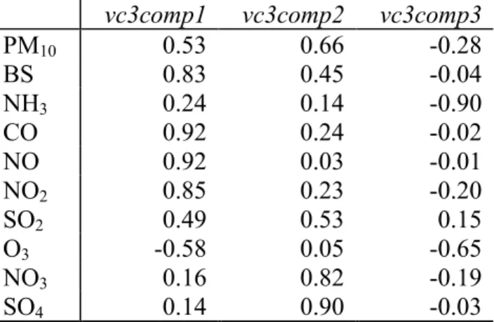
As mentioned before, we would like to use the principal components as summary of the air pollution data: we want to include only the first principal components (or eventually rotations of these components) as explanatory variables in mortality analyses. Since the last principal components have relatively small variances, it is unlikely that we lose important information by excluding these variables. The question is how many principal components to retain and whether a rotation should be carried out. The idea of a rotation is that we choose new co-ordinates (which are a rotation of the first standardised principal components), such that the rotated components span the same subspace as the original first standardised principal components (in that sense, they contain the same information). The purpose of rotation is that we hope to find variables that have an interpretation in terms of different sources of air pollution. For a detailed explanation of rotations, we refer to Chapter 5 of Basilevsky (1994). We examine the correlation loadings of the first components (see Table 5), but we cannot interpret these components as representing certain sources of air pollution. We therefore decide to apply a varimax rotation on the first three standardised principal components. We want to achieve that some of the new correlation loadings will be relatively large, while other loadings will be relatively small. This might simplify the interpretation of the various components. In the case of the varimax rotation on the first three standardised principal components, the rotation is chosen for which the sum of the variances of the new first three squared correlation loadings is maximal (see Basilevsky 1994 p. 263). In Splus, this rotation is obtained by choosing the option normalize=F in the rotate command. We denote the rotated components by vc3comp1, vc3comp2 and vc3comp3, to express that these are the result of the varimax rotation of the correlation loadings of the first 3 standardised principal components.

The correlation loadings of the varimax rotation of the first three standardised components can be found in Table 7 below.

Table 7 Correlation loadings after a varimax rotation of the first three standardised principal components

vc3comp1 vc3comp2 vc3comp3

PM10 0.53 0.66 -0.28 BS 0.83 0.45 -0.04 NH3 0.24 0.14 -0.90 CO 0.92 0.24 -0.02 NO 0.92 0.03 -0.01 NO2 0.85 0.23 -0.20 SO2 0.49 0.53 0.15 O3 -0.58 0.05 -0.65 NO3 0.16 0.82 -0.19 SO4 0.14 0.90 -0.03

The rotated components vc3comp1, vc3comp2 and vc3comp3 have variance 1, are mutually uncorrelated and also uncorrelated with *

4

PC up to *

10

PC (inclusive). To make things clearer,

(19)

. 08 . 0 09 . 0 05 . 0 02 . 0 34 . 0 18 . 0 18 . 0 3 3 28 . 0 2 3 66 . 0 1 3 53 . 0 * 10 * 9 * 8 * 7 * 6 * 5 * 4 10 PC PC PC PC PC PC PC comp vc comp vc comp vc PM + + − − − − + − + =

When we consider the correlation loadings of the rotated components, we see that vc3comp1 is highly correlated with the pollutants BS, CO, NO and NO2 andmoderately correlated with

PM10 and O3. This might indicate a relation with traffic emissions. The second and third

rotated component cannot be associated to different categories of air pollution. We decided that these rotated components are not (all) interpretable as source-related variables. We therefore apply a varimax rotation on the first four standardised principal components, to see whether this leads to a more interpretable result. The corresponding correlation loadings are displayed in Table 8.

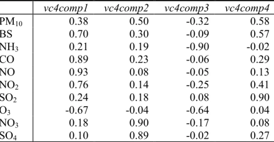
Table 8 Varimax rotation of the first four standardised principal components (correlation loadings)

vc4comp1 vc4comp2 vc4comp3 vc4comp4

PM10 0.38 0.50 -0.32 0.58 BS 0.70 0.30 -0.09 0.57 NH3 0.21 0.19 -0.90 -0.02 CO 0.89 0.23 -0.06 0.29 NO 0.93 0.08 -0.05 0.13 NO2 0.76 0.14 -0.25 0.41 SO2 0.24 0.18 0.08 0.90 O3 -0.67 -0.04 -0.64 0.04 NO3 0.18 0.90 -0.17 0.08 SO4 0.10 0.89 -0.02 0.27

The correlations between the concentrations and vc4comp1 resemble the situation of vc3comp1 and we can interpret this again as traffic. The second component, vc4comp2, is highly correlated with NO3 an SO4, which are secondary aerosols. The third component,

vc4comp3, is strongly correlated with NH3, which might suggest a relation with bio-industry,

but the relatively strong correlation with O3 is not expected for a component representing

bio-industry. The last component, vc4comp4, is highly correlated with SO2 and moderately with

PM10 and BS, we could interpret this as industrial sources.

We finally rotate the first five standardised principal components, to see whether this makes the picture clearer. The results can be found in table 9.The rotated components are denoted by vc5comp1 up to vc5comp5.

Table 9 with five uncorrelated components presents the most promising results to use for the mortality analysis. An interpretation of the various components will be presented according to the structure of the emissions of the different source categories that can be discerned in the Netherlands. Concerning the correlation structure of the air pollution concentrations, we must realise that stemming from the same source is not the only reason for the observed interrelationships between pollutant concentrations. A number of modulating factors must be taken into account. The foremost important factor will be large-scale meteorology that governs transport of pollution and controls the dispersion and removal. On a smaller scale also diurnal modulation plays a role, because of differences in source patterns and temporal profiles of source categories influence the correlation pattern. One of the other factors we have to consider is the influence of seasons, as a number of air polluting components in the

(20)

Netherlands have a seasonal pattern that differs from the rest of the components. In this light it might seem illogical to search for uncorrelated components to represent the different

sources of air pollution. Nevertheless we think that we can give a meaningful interpretation of the five varimax-rotated components and that it is worthwhile to use these components as explanatory variables in a mortality analysis.

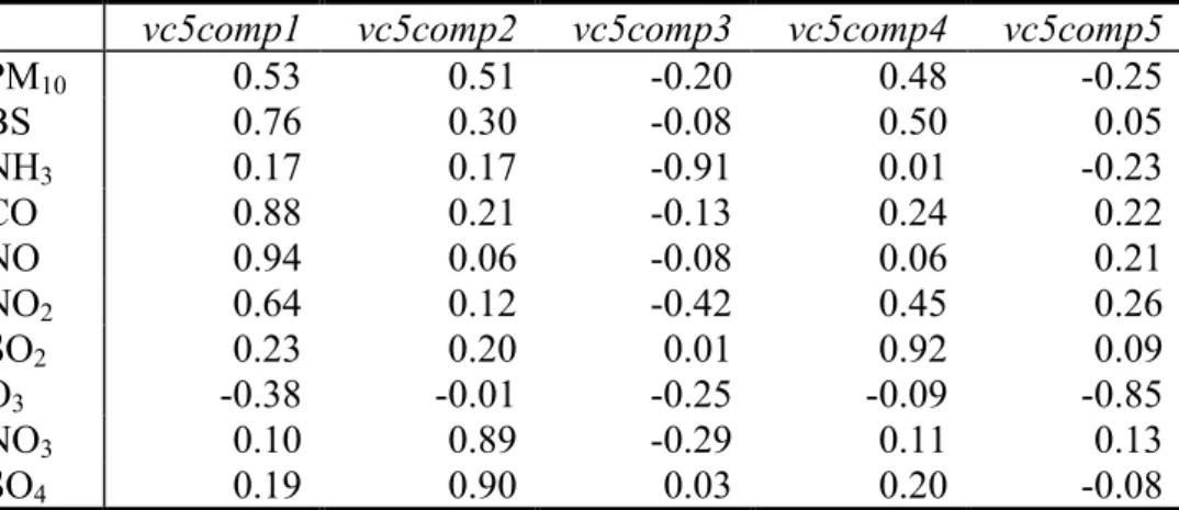
Table 9 Varimax rotation of the first five standardised principal components (correlation loadings)

vc5comp1 vc5comp2 vc5comp3 vc5comp4 vc5comp5

PM10 0.53 0.51 -0.20 0.48 -0.25 BS 0.76 0.30 -0.08 0.50 0.05 NH3 0.17 0.17 -0.91 0.01 -0.23 CO 0.88 0.21 -0.13 0.24 0.22 NO 0.94 0.06 -0.08 0.06 0.21 NO2 0.64 0.12 -0.42 0.45 0.26 SO2 0.23 0.20 0.01 0.92 0.09 O3 -0.38 -0.01 -0.25 -0.09 -0.85 NO3 0.10 0.89 -0.29 0.11 0.13 SO4 0.19 0.90 0.03 0.20 -0.08

The first component, vc5comp1, can be interpreted as a component associated to traffic emissions for reasons elaborated below. This component is correlated highest with NO (a correlation of 0.94 in Table 9). This is also the principal fraction that is emitted by traffic, approximately 80-90% of the NOx emissions of traffic is emitted directly as NO, which

afterwards gets transformed into NO2 quite quickly and eventually into NO3- by a number of

secondary inorganic reaction steps. In a component representing traffic, we expect that this is expressed by the magnitude of the correlations with NO2 and NO3-, we expect that the

correlation with NO2 is substantial, but the correlation with NO3- could be pretty low. We see

such a pattern in vc5comp1: the component has a correlation of 0.64 with NO2 and of 0.10

with NO3-. The second most important correlation with vc5comp1 is with CO: 0.88, which

also is an important indicator of traffic. The third largest correlation is with BS (0.76), which is also in line with traffic as a dominant source. Most of the particulate traffic emissions are from diesel engines and comprise carbonaceous PM of a sooty character that is easily captured by BS measurements. The influence of traffic on the BS levels in the Netherlands is considerably larger than that on PM10 in general, which fits with a lower correlation of

vc5comp1 with PM10 (0.53) than with BS.

RIVM (1996) reports that in 1995 the total Dutch NOx emissions were 518 kT/y, of which

334 kT was from traffic. The other important sources of NOx emissions were energy

production 60 kT and industry + refineries 78 kT in 1995. One could therefore argue that the correlation in a traffic-related component with NO is not expected to be as high as in vc5comp1. On the other hand, the last two source categories (energy and industry + refineries) are supposed to have a somewhat different diurnal profile than that of traffic. These source categories possibly have a more continuous character of operation, such that fluctuations in the concentration of NOx might be mostly attributable to traffic, though the

contribution of industry and refineries in absolute terms to the NOx emissions is by no means

negligible.

For the second largest correlation (between vc5comp1 and CO) a similar reasoning can be presented. The total Dutch emissions in 1995 were 873kT/y of CO. Of this amount 518 kT of CO was from traffic and 228 kT of CO was emitted by industry in 1995 (RIVM, 1996).

(21)

The second component, vc5comp2, is dominated by high correlation loadings with sulphate and nitrate. This component can be characterised as the result of inorganic transformations, as the end products of secondary aerosol formation from the precursor gases SO2 and NOx are

the main factors driving the correlation structure for v5comp2. Sulphate and nitrate still are an important part of the total PM10 in the Netherlands; in 1995 slightly more than 20% of

regional Dutch PM10 levels was either sulphate or nitrate (Den Hartog et al. (1997)).

Therefore we expect that in a component representing inorganic transformations also the correlation with PM10 will be not negligible. This is exactly what we see in vc5comp2: a

correlation of 0.51 with PM10. The correlation between vc5comp2 and BS is quite low (0.30).

This does not conflict with an interpretation of vc5comp2 as representing inorganic transformations, since sulphate and nitrate are no part of BS, while being a considerable part of PM10.

This vc5comp2 can not be directly related to emissions in the Netherlands, as inorganic secondary aerosol formation is a process that takes time and local ambient concentrations of especially sulphate are for the larger part (95%) dominated by foreign transport. Also for this reason the interrelationship with the local Dutch concentrations of the precursor gases (SO2

and NO2) is expected to be lower than of the previously mentioned components of PM.

The third component, vc5comp3, has its main correlation loading (-0.91) with NH3 and none

of the other components. This seems to point to a source as agriculture or bio-industry. In the Netherlands the yearly emissions of NH3 in 1995 were 155 kT/y, of which 144 kT originated

by agriculture (RIVM, 1996). For none of the other air pollution components the source category agriculture is an important contributor, so the fact that all correlations with other pollutants are low, fits with an interpretation of vc5comp3 as representing bio-industry. Maybe only the correlation with NO2 is a bit stronger than expected.

In the Netherlands the concentrations of NH3 are more a local phenomenon than

concentrations of any of the other primary air pollution components, and foreign contribution of NH3 is only of secondary importance in our country. In 1995 approximately 6% of PM10

was NH4+ (Den Hartog et al., 1997), the secondary product of NH3 after neutralisation, while

none of the BS was NH4+ or possibly only slightly NH3 related. Possibly vc5comp3 can also

be related to seasonal activities and sources of PM that are related to agricultural activities as haying, harvesting and combining, also these sources tend to peak primarily during summer in the Netherlands. See also Table 32, the mean of vc5comp3 is negative in summer and positive in winter, which points to an average pollution level that is higher in summer than in winter (since the most important correlations with vc5comp3 are negative).

The fourth component vc5comp4 has its highest correlation loading with SO2 (0.92). This

might be somewhat of a surprise as the emissions of SO2 have decreased considerably in the

Netherlands during the past decades. But one should realise that it is not the absolute height of the concentrations or the emissions but the correlation structure that is the driving force behind the components that are found in the principal components analysis (since we use standardised concentrations). In 1995 the total emission of SO2 was 147 kT/y, of which

industry + refineries contributed 94 kT and energy production 18 kT (RIVM, 1996). The traffic contribution was 30kT. Therefore we interpret vc5comp4 as reflecting industrial sources and more in particular those industrial sources or continuously working energy production related sources that have a temporal emission structure that is different from that of traffic. The moderate correlation of vc5comp4 and BS (0.50) and PM10 (0.48) also points

(22)

in the direction of industrial sources: of the total PM10 emission of 60kT/y in 1995 in the

Netherlands (Buringh et al., 2002) the industrial and traffic contribution to the primary PM10

emission was 21 kT each. The very small correlation loading of vc5comp4 with NO seems illogical for a component representing industry, but as we mentioned earlier, fluctuations in NOx might be mainly driven by traffic emissions.

Finally, vc5comp5 has its strongest correlation loading (-0.85) with ozone, this points to some photochemical processes behind this component. These processes occur more in summer than in winter and we therefore expect the mean of this component to be negative in summer and positive in winter (since the correlation with ozone is negative). This is indeed what we see in Table 32 of the Appendix, the mean is approximately –0.6 in the summer and 0.5 in the winter. Part of PM10, though in the Netherlands the magnitude of this part is

unknown, probably is related to ozone by way of secondary organic aerosol formation (SOA). This might explain a similar sign between the photochemical factor vc5comp5 and PM10. Because ozone is not emitted into the air directly, this vc5comp5 cannot be compared

with emissions from Dutch sources.

A summary of our interpretation of the components is presented in Table 10 below.

Table 10 Interpretation of the components

component Source

vc5comp1 Traffic related

vc5comp2 Secondary inorganic transformations vc5comp3 Bio-industry

vc5comp4 Industry related

vc5comp5 Photochemical transformations

The loadings for the varimax rotation of the first five standardised components as linear combination of the air pollution concentrations can be found in Table 11.

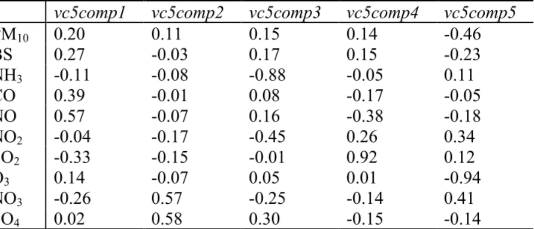
Table 11 Loadings of the varimax rotation of the first five standardised components as linear combination of the standardised concentrations

vc5comp1 vc5comp2 vc5comp3 vc5comp4 vc5comp5

PM10 0.20 0.11 0.15 0.14 -0.46 BS 0.27 -0.03 0.17 0.15 -0.23 NH3 -0.11 -0.08 -0.88 -0.05 0.11 CO 0.39 -0.01 0.08 -0.17 -0.05 NO 0.57 -0.07 0.16 -0.38 -0.18 NO2 -0.04 -0.17 -0.45 0.26 0.34 SO2 -0.33 -0.15 -0.01 0.92 0.12 O3 0.14 -0.07 0.05 0.01 -0.94 NO3 -0.26 0.57 -0.25 -0.14 0.41 SO4 0.02 0.58 0.30 -0.15 -0.14

The daily values of the components are easily computed with the loadings in Table 11. We also constructed the lag 1 day, lag 2 days and lag 3 days variables of the components and the average value of the components in the preceding week (which is the average of lag 1 up to and including lag 7). The lag-variables are successively denoted by l1, l2, l3 or wk after the name of the rotated principal component.

(23)

2.5 Conclusion Part one:

In our opinion, the variables vc5comp1 up to vc5comp 5, which result from a varimax rotation of the first five standardised principal components, are appropriate to be used as source related explanatory variables in a mortality analysis. The correlation structure of these components and the air pollution concentrations is presented in Table 9 and our interpretation in Table 10. We will use these variables and the corresponding lag-variables as source related explanatory variables for mortality in Part two of this study.

(24)

(25)

3 Part two: Associations between mortality and the five

varimax rotated standardised principal components

3.1 Overview

In Part one, we extracted five readily interpretable components after principal component analyses (PCA) with varimax rotation from a time series of air pollution data. As mentioned in the conclusion of Part one, we think the correlation structure of these vc5comp1 up to vc5comp5 (see Table 9) makes it worthwhile to use these variables (and the associated lag-variables) as explanatory variables for daily mortality. Recall that our interpretation of these components can be found in Table 10.

The association between these components and mortality is modelled with a generalised additive model (GAM), in one- and multi-component models. In these models also a large number of confounding variables is included, to correct for meteorological influences, influenza epidemics, time of the year etc. We call the models with only the confounding variables base-models. We also fit models in which the rotated components interact with the season. In this part of the report, we will first describe the data and the computer programs used. Then we will describe the method and the base-model and we present the results.

3.2 Data

3.2.1 Rotated principal components

We use the five varimax rotated principal components vc5comp1, vc5comp2, vc5comp3, vc5comp4, vc5comp5 and the associated lags as described in Part one of this report.

For a more detailed description of the further data, the origin of the data and the data collection, we refer to Fischer et al. (in preparation). In that study the same data are used (but during a longer period). We here only shortly list the variables used for this study (period 1993-1998).

3.2.2 Mortality data

These data are obtained from the Central Bureau of Statistics (CBS) and do not include deaths of Dutch citizens who died outside the Netherlands and non-residents who died inside the Netherlands, nor deaths for whom the exact date of death was unknown. Also deaths due to accidents were excluded. We use the following categories:

• Daily total mortality (ICD-9 <800)

• Daily respiratory mortality (ICD-9 460-519) • Daily pneumonia mortality (ICD-9 480-486)

• Daily chronic obstructive disease (COPD) mortality (ICD-9 490-496) • Daily cardiovascular diseases mortality (ICD-9 390-448)

(26)

3.2.3 Meteorological data

We use daily averages of temperature, relative humidity and barometric pressure, averaged over the Netherlands. Meteorological data were obtained from the Royal Dutch Meteorological Institute (KNMI).

3.2.4 Influenza

We use data on influenza morbidity (obtained from the Dutch Institute for Research of Health care in Utrecht). For each day we have three variables, namely an estimate of the weekly average of influenza morbidity of the past week (lag 0-6 days), the week before the past week (lag 7-13 days) and two weeks before the past week (lag 14-20 days).

3.2.5 Pollen

We use data on airborne pollen obtained through Dr. Spieksma (Hospital Leiden). In this study we use pollen counts of Rumex, Betula and Poacea.

3.3 Software

We use Splus 2000 (for Windows) and Splus 6.0 (for UNIX) to perform the GAM analyses and to compute correlations and quantiles. Relative risks are computed with Microsoft Excel 97.

3.4 Method and base models

3.4.1 Generalised additive models

As is usual (Samet, 2002) in epidemiological studies on associations between air pollution and mortality, we used Generalised Additive Models (GAM) to estimate associations between the (lags of) rotated principal components and the five mortality variables: total, respiratory, cardiovascular diseases, pneumonia and COPD mortality. For a detailed description of generalised additive models we refer to Hastie and Tibshirani (1990).

We use the built-in GAM function of Splus. As reported in Dominici et al. (2002), there are some problems with the default settings of the convergence parameters of this function. We therefore use the new control parameters communicated by Trevor Hastie via the s-news list: the convergence threshold for local scoring iterations and for back fitting iterations is set to

7

10− _{, the maximum number of scoring iterations and of back fitting iterations is set to 30. In} a generalised additive model for mortality one usually uses a Poisson family and corrects standard errors for overdispersion, but Splus obtains the same effect estimates when we use a quasi likelyhood family (family=quasi(link=log, var=’mu’)), while the standard errors are the corrected ones, so we used this family.

To simplify interpretation, the rotated principal components are fitted linearly in the models. We include functions of confounding variables, to adjust for date (to incorporate seasonal and long-term trends), influenza, temperature, relative humidity, atmospheric pressure, day of the week, holidays and pollen. Some of these variables were included linearly in the models,

(27)

others with loess smoothers, polynomial splines, with values for different categories of the data, or as factor. As mentioned in Fischer et al. (in preparation), the technique of loess smoothing can be seen as an advanced version of using moving averages. In loess smoothing a span is involved, that is a parameter indicating the fraction of the range of the data that is used in the smoother. We use the same base models as in Fischer et al. (in preparation), which will be described later. We start with one-component models in which only one rotated principal component is used as explanatory variable (together with the confounding variables of the base models) later we also fit multi-component models.

To estimate the influence of the season on the effects, we also fit models in which the rotated principal components are fitted in interaction with the season. We also fit one-component models with the original (not rotated) principal components.

Relative risks

To make the effect estimates easier to interpret, we computed relative risks. We compared the risk at the 95%-quantile of the component by the risk at the 5%-quantile for the variables vc5comp1, vc5comp2 and vc5comp4. For vc5comp3 and vc5comp5 we compared the risk at the 5%-quantile by the risk at the 95-quantile, since for these components negative values generally correspond to days with high air pollution concentrations (see also Table 11, the largest loadings are negative). We also computed the 95% lower confidence limits of the relative risks (RR-lo) and the 95% upper confidence limits of the relative risks (RR-hi).

3.4.2 Base models

As indicated earlier, we use the same base-models as in Fischer et al. (in preparation), since in that study almost the same data set is used: there is only one extra year involved, 1992, that is excluded from our analysis because of many missing values for NH3. For this reason we

make an adjustment for the loess functions of date included in the base models: we multiply the spans used in Fischer et al. (in preparation) by 7/6, to correct for the shorter time-period used in the current study (six instead of seven years). For details on the construction of the base models we refer to Fischer et al. (in preparation), we limit ourselves here to the description of the final base models.

For total mortality the base model is made up of the following functions: • a loess smoother of the date with a span of 0.03×7/6

• a loess smoother of the average influenza morbidity of the past week with a span of 0.8 • a linear function of the average influenza morbidity of two weeks before the past week • a loess smoother of the temperature with a span of 0.6

• a loess smoother of lag 2 of the temperature with a span of 0.6

• a polynomial spline function (of degree 1) with 70 knots of lag 2 of the relative humidity • a linear function of the barometric pressure

• a piecewise constant function of lag 2 of the pollen counts of Poacea with jumps at -1, 21, 77, 135 and 10000

• a piecewise constant function of lag 2 of the pollen counts of Betula with jumps at -1, 17, 68, 600 and 10000

• a piecewise constant function of lag 2 of the pollen counts of Rumex with jumps at -1, 5 and 10000

• a factor function of the day of the week (that comes down to adding a different constant for each day of the week)

(28)

• a linear function of holidays (that comes down to adding a constant in periods of holidays, since holidays are represented by an indicator variable)

For respiratory mortality the base model consists of: • a loess smoother of the date with a span of 0.03×7/6

• a linear function of the average influenza morbidity of the past week

• a loess smoother of the influenza morbidity of the week before the past week with a span of 0.9

• a loess smoother of lag 1 of the temperature with a span of 0.8 • a loess smoother of lag 3 of the temperature with a span of 0.8

• a polynomial spline function (of degree 1) with 70 knots of lag 1 of the relative humidity • a linear function of the barometric pressure

• a factor function of the day of the week • a linear function of holidays

For cardiovascular diseases mortality the base model is made up of: • a loess smoother of the date with a span of0.04×7/6

• a loess smoother of the average influenza morbidity of the past week with a span of 0.7 • a loess smoother of lag 1 of the temperature with a span of 0.5

• a loess smoother of lag 2 of the temperature with a span of 0.5 • a linear function of the relative humidity

• a linear function of barometric pressure

For pneumonia mortality, the base model is composed of: • a loess smoother of date with a span of 0.04×7/6

• a loess smoother of the average influenza morbidity of the past week with a span of 0.9 • a loess smoother of the average influenza morbidity of two weeks before the past week

with a span of 0.9

• a loess smoother of lag 1 of the temperature with a span of 0.8 • a loess smoother of lag 3 of the temperature with a span of 0.8 • a loess smoother of lag 1 of the relative humidity with a span of 1 • a loess smoother of the barometric pressure with a span of 1

(29)

For COPD mortality we used the following functions in the base model: • a loess smoother of date with a span of 0.04×7/6

• a linear function of the average influenza morbidity of the past week

• a loess smoother of the average influenza morbidity of a week before the past week with a span of 0.6

• a loess smoother of the temperature with a span of 0.8

• a loess smoother of lag 2 of the temperature with a span of 0.8 • a linear function of the relative humidity

• a linear function of the barometric pressure

(30)

3.5 Results

3.5.1 Associations with the five varimax rotated principal components:

one-component models

To quantify the associations between the rotated principal components and the five mortality variables, we first add one component (lag 0, 1, 2, 3 or the average of the lags 1-7) to the base models. The components are added as a linear function, to simplify interpretation. That is, we fit a generalised additive model with confounding variables as in the base models and a linear function of (a lag of) a component.

Table 12 gives the quantiles of the rotated components, which are used to compute relative risks. In the column 90% range, the difference between the 95%-quantile and the 5%-quantile is displayed. Quantiles of the lag 1, 2 and 3 variables are (almost) equal to the quantiles of the corresponding lag 0 variables and are therefore omitted.

Table 12 Quantiles of the five varimax rotated principal components

Component 5% quantile 95% quantile 90% range

vc5comp1 -0.83 2.02 2.85 vc5comp1wk -0.57 1.49 2.06 vc5comp2 -1.12 1.80 2.92 vc5comp2wk -0.74 1.19 1.93 vc5comp3 -1.80 1.25 3.05 vc5comp3wk -1.35 0.93 2.28 vc5comp4 -0.98 1.58 2.56 vc5comp4wk -0.67 1.12 1.78 vc5comp5 -1.86 1.35 3.21 vc5comp5wk -1.73 1.01 2.74

In Table 13 up to Table 17 below, the results of the one-component models are presented, significant results are highlighted. For the effect measure, realise that the fitted models look like: s confounder of functions value component effect deaths of number )= ∗ + ln(

Therefore the relative risks are computed as: )

% 90

exp(effect range

RR= ∗± ) % 90 ) . 96 . 1

exp((effect sterror range lo RR− = − ∗ ∗± ) % 90 ) . 96 . 1

exp((effect sterror range hi

RR− = + ∗ ∗± ,

here the sign for the 90% range is taken positive for the components vc5comp1, vc5comp2 and vc5comp4, and negative for vc5comp3 and vc5comp5 (for all lags). For reasons of presentation and interpretation, we changed the original signs of the regression coefficients and t-values from the GAM-analyses for the components vc5comp3 and vc5comp5.

(31)

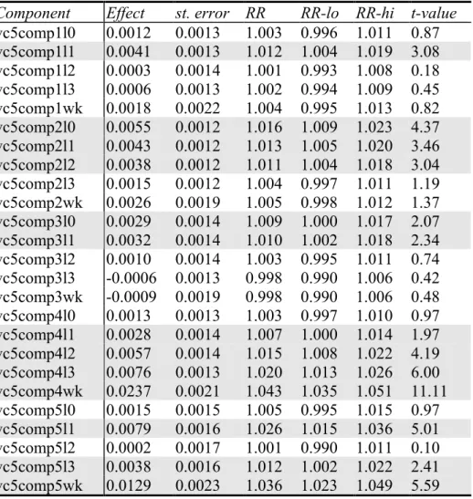
Table 13 one-component models for total mortality

Component Effect st. error RR RR-lo RR-hi t-value

vc5comp1l0 0.0012 0.0013 1.003 0.996 1.011 0.87 vc5comp1l1 0.0041 0.0013 1.012 1.004 1.019 3.08 vc5comp1l2 0.0003 0.0014 1.001 0.993 1.008 0.18 vc5comp1l3 0.0006 0.0013 1.002 0.994 1.009 0.45 vc5comp1wk 0.0018 0.0022 1.004 0.995 1.013 0.82 vc5comp2l0 0.0055 0.0012 1.016 1.009 1.023 4.37 vc5comp2l1 0.0043 0.0012 1.013 1.005 1.020 3.46 vc5comp2l2 0.0038 0.0012 1.011 1.004 1.018 3.04 vc5comp2l3 0.0015 0.0012 1.004 0.997 1.011 1.19 vc5comp2wk 0.0026 0.0019 1.005 0.998 1.012 1.37 vc5comp3l0 0.0029 0.0014 1.009 1.000 1.017 2.07 vc5comp3l1 0.0032 0.0014 1.010 1.002 1.018 2.34 vc5comp3l2 0.0010 0.0014 1.003 0.995 1.011 0.74 vc5comp3l3 -0.0006 0.0013 0.998 0.990 1.006 0.42 vc5comp3wk -0.0009 0.0019 0.998 0.990 1.006 0.48 vc5comp4l0 0.0013 0.0013 1.003 0.997 1.010 0.97 vc5comp4l1 0.0028 0.0014 1.007 1.000 1.014 1.97 vc5comp4l2 0.0057 0.0014 1.015 1.008 1.022 4.19 vc5comp4l3 0.0076 0.0013 1.020 1.013 1.026 6.00 vc5comp4wk 0.0237 0.0021 1.043 1.035 1.051 11.11 vc5comp5l0 0.0015 0.0015 1.005 0.995 1.015 0.97 vc5comp5l1 0.0079 0.0016 1.026 1.015 1.036 5.01 vc5comp5l2 0.0002 0.0017 1.001 0.990 1.011 0.10 vc5comp5l3 0.0038 0.0016 1.012 1.002 1.022 2.41 vc5comp5wk 0.0129 0.0023 1.036 1.023 1.049 5.59

(32)

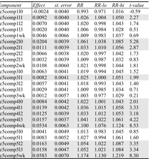
Table 14 one-component models for respiratory mortality

vc5comp1l0 -0.0024 0.0040 0.993 0.971 1.016 -0.59 vc5comp1l1 0.0092 0.0040 1.026 1.004 1.050 2.27 vc5comp1l2 0.0070 0.0040 1.020 0.998 1.043 1.74 vc5comp1l3 0.0020 0.0040 1.006 0.984 1.028 0.51 vc5comp1wk 0.0046 0.0066 1.009 0.983 1.037 0.69 vc5comp2l0 0.0204 0.0039 1.061 1.038 1.085 5.28 vc5comp2l1 0.0111 0.0039 1.033 1.010 1.056 2.87 vc5comp2l2 0.0066 0.0038 1.020 0.997 1.042 1.73 vc5comp2l3 0.0032 0.0039 1.009 0.987 1.032 0.83 vc5comp2wk 0.0108 0.0060 1.021 0.998 1.044 1.81 vc5comp3l0 0.0063 0.0041 1.019 0.994 1.045 1.52 vc5comp3l1 0.0082 0.0041 1.025 1.000 1.051 1.99 vc5comp3l2 0.0057 0.0041 1.018 0.993 1.043 1.40 vc5comp3l3 0.0029 0.0041 1.009 0.985 1.034 0.71 vc5comp3wk 0.0012 0.0057 1.003 0.977 1.029 0.21 vc5comp4l0 0.0084 0.0042 1.022 1.001 1.043 2.01 vc5comp4l1 0.0139 0.0042 1.036 1.015 1.058 3.33 vc5comp4l2 0.0125 0.0039 1.033 1.012 1.053 3.18 vc5comp4l3 0.0157 0.0037 1.041 1.022 1.061 4.22 vc5comp4wk 0.0534 0.0063 1.100 1.076 1.124 8.53 vc5comp5l0 0.0041 0.0049 1.013 0.983 1.045 0.85 vc5comp5l1 0.0083 0.0052 1.027 0.994 1.061 1.60 vc5comp5l2 0.0163 0.0049 1.054 1.022 1.087 3.35 vc5comp5l3 0.0158 0.0047 1.052 1.021 1.084 3.34 vc5comp5wk 0.0583 0.0070 1.174 1.130 1.219 8.30

(33)

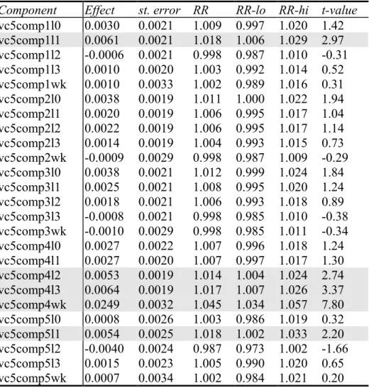
Table 15 one-component models for cardiovascular diseases mortality

vc5comp1l0 0.0030 0.0021 1.009 0.997 1.020 1.42 vc5comp1l1 0.0061 0.0021 1.018 1.006 1.029 2.97 vc5comp1l2 -0.0006 0.0021 0.998 0.987 1.010 -0.31 vc5comp1l3 0.0010 0.0020 1.003 0.992 1.014 0.52 vc5comp1wk 0.0010 0.0033 1.002 0.989 1.016 0.31 vc5comp2l0 0.0038 0.0019 1.011 1.000 1.022 1.94 vc5comp2l1 0.0020 0.0019 1.006 0.995 1.017 1.04 vc5comp2l2 0.0022 0.0019 1.006 0.995 1.017 1.14 vc5comp2l3 0.0014 0.0019 1.004 0.993 1.015 0.73 vc5comp2wk -0.0009 0.0029 0.998 0.987 1.009 -0.29 vc5comp3l0 0.0038 0.0021 1.012 0.999 1.024 1.84 vc5comp3l1 0.0025 0.0021 1.008 0.995 1.020 1.24 vc5comp3l2 0.0018 0.0021 1.006 0.993 1.018 0.89 vc5comp3l3 -0.0008 0.0021 0.998 0.985 1.010 -0.38 vc5comp3wk -0.0010 0.0029 0.998 0.985 1.011 -0.34 vc5comp4l0 0.0027 0.0022 1.007 0.996 1.018 1.24 vc5comp4l1 0.0027 0.0020 1.007 0.997 1.017 1.30 vc5comp4l2 0.0053 0.0019 1.014 1.004 1.024 2.74 vc5comp4l3 0.0064 0.0019 1.017 1.007 1.026 3.37 vc5comp4wk 0.0249 0.0032 1.045 1.034 1.057 7.80 vc5comp5l0 0.0008 0.0026 1.003 0.986 1.019 0.32 vc5comp5l1 0.0054 0.0025 1.018 1.002 1.033 2.20 vc5comp5l2 -0.0040 0.0024 0.987 0.973 1.002 -1.66 vc5comp5l3 0.0015 0.0023 1.005 0.990 1.020 0.65 vc5comp5wk 0.0007 0.0034 1.002 0.984 1.021 0.20

(34)

Table 16 one-component models for pneumonia mortality

Component Effect st.error RR RR-lo RR-hi t-value

vc5comp1l0 0.0079 0.0063 1.023 0.988 1.059 1.26 vc5comp1l1 0.0216 0.0062 1.064 1.028 1.101 3.50 vc5comp1l2 0.0107 0.0062 1.031 0.996 1.068 1.73 vc5comp1l3 0.0038 0.0062 1.011 0.976 1.046 0.61 vc5comp1wk -0.0058 0.0103 0.988 0.948 1.030 -0.57 vc5comp2l0 0.0166 0.0061 1.050 1.014 1.087 2.73 vc5comp2l1 0.0063 0.0061 1.018 0.983 1.055 1.02 vc5comp2l2 0.0008 0.0061 1.002 0.968 1.038 0.13 vc5comp2l3 -0.0070 0.0061 0.980 0.946 1.015 -1.14 vc5comp2wk 0.0159 0.0093 1.031 0.995 1.068 1.71 vc5comp3l0 0.0234 0.0064 1.074 1.034 1.116 3.64 vc5comp3l1 0.0166 0.0064 1.052 1.013 1.093 2.61 vc5comp3l2 0.0113 0.0064 1.035 0.996 1.076 1.78 vc5comp3l3 0.0051 0.0064 1.016 0.978 1.055 0.80 vc5comp3wk 0.0112 0.0089 1.026 0.986 1.067 1.25 vc5comp4l0 0.0099 0.0065 1.026 0.993 1.060 1.52 vc5comp4l1 0.0154 0.0065 1.040 1.007 1.075 2.35 vc5comp4l2 0.0191 0.0061 1.050 1.018 1.083 3.12 vc5comp4l3 0.0224 0.0058 1.059 1.029 1.091 3.87 vc5comp4wk 0.0690 0.0096 1.131 1.094 1.170 7.18 vc5comp5l0 0.0028 0.0076 1.009 0.962 1.058 0.37 vc5comp5l1 0.0131 0.0081 1.043 0.991 1.097 1.62 vc5comp5l2 0.0287 0.0075 1.096 1.046 1.149 3.81 vc5comp5l3 0.0368 0.0073 1.125 1.075 1.178 5.06 vc5comp5wk 0.0989 0.0108 1.312 1.238 1.390 9.16