of the EMEP Unified (Eulerian) model
G.J.M. Velders, E.S. de Waal, J.A. van Jaarsveld, J.F. de Ruiter
This investigation was performed by order and for the account of the Directorate-General for Environmental Protection (DGM/KvI) of the Netherlands' Ministry of Housing, Spatial Planning and the Environment, within the framework of project M/500037 "Nationaal Luchtbeleid", Milestone "EMEP model evaluation".
Abstract
A few aspects of the EMEP Unified (Eulerian) model have been evaluated by analysing the deposition parameterisation for acidifying compounds and the concentration and deposition of SOx, NOx, and NHx in the Netherlands. Evaluation was also carried out by analysing the
source-receptor matrices for the Netherlands and the geographical distribution of the emissions, comparing results with both the OPS model and measurements. The picture given of the Netherlands by the EMEP Unified model was found for most acidifying compounds to be a fair one. The source-receptor matrices calculated by the EMEP and OPS models were seen to be in good agreement for oxidised sulphur, and in reasonable agreement for reduced nitrogen. Large discrepancies between the models were found for oxidised nitrogen. The contribution of the Dutch emissions to local deposition in the Netherlands came to a factor of 4 higher in the OPS model, compared to the EMEP model. The contributions of Belgium and Germany to deposition are also much higher in the OPS model. These differences can be traced back to the lower concentration and dry deposition, along with higher wet deposition, of NOx in the EMEP model. For oxidised nitrogen, there was a large difference in the
influence of the boundary and initial conditions on the source-receptor matrix. The EMEP model suggests that almost 30% of the deposition is due to sources outside Europe. The SO2
concentrations in the Netherlands calculated with the EMEP model are close to the measurements, while the NOx concentrations are about 40% lower and the NH3
Preface
EMEP model output is used as input in the RAINS model, which, in turn, forms an important element of the scientific base for policy measures in the EU Clean Air for Europe (CAFE) programme and in the framework of the UNECE Convention on Long-Range Transboundary Air Pollution (CLRTAP). This report represents the results of evaluating the EMEP Unified model, as commissioned by the EMEP’s Task Force on Measurements and Modelling (TFMM) through the EMEP Steering Body. The aim of the evaluation was to address the suitability of the model for assessing regional concentrations and long-range transboundary fluxes of sulphur, oxidised and reduced nitrogen, VOCs, ozone and suspended particulate matter. The activities described represent the RIVM-MNP contribution to the EMEP model’s evaluation, intended to contribute to the quality of the EMEP model and the source-receptor matrices, and to assist in the policy-making process.
Contents
Executive Summary 5
Samenvatting 7
1. Introduction 9
2. Deposition parameterisation 11
2.1 Comparison of overall dry deposition velocities EMEP and OPS 12
2.2 General comments on dry deposition parameterisations 15
3. EMEP versus OPS on a 50 x 50 km grid 16
4. Source-receptor relationships for the Netherlands 22
5. Distribution of emissions 26
6. Discussion 30
Literature 31
Executive Summary
A selected set of analyses has been performed by RIVM-MNP to evaluate the EMEP Unified (Eulerian) model. The analyses concentrated on the deposition parameterisation for acidifying compounds, the concentration and deposition of SOx, NOx, and NHx in the
Netherlands, the source-receptor matrices for the Netherlands and the geographical distribution of the emissions. For the evaluation, EMEP results were compared both with the OPS results and observations in the Netherlands to yield the following conclusions for the EMEP Unified model:
• The EMEP Unified model was concluded to give a fair picture of the concentration
and deposition of most acidifying compounds in the Netherlands. Source-receptor matrices
• The source-receptor matrices for oxidised sulphur (SOx) calculated by the EMEP
and OPS models are in good agreement. The agreement for reduced nitrogen (NHx)
is reasonable. For reduced nitrogen, the EMEP model calculated a higher contribution to
the deposition in the Netherlands from emissions in Belgium and Germany, and a lower contribution from the Netherlands.
• Large discrepancies between the EMEP and OPS models were found in the
source-receptor matrices for oxidised nitrogen (NOy). The local deposition contribution of the
Dutch emissions to the deposition in the Netherlands comes to a factor of 4 higher in the OPS model than in the EMEP model. The Dutch emissions contribute only 8% to the deposition in the Netherlands. This was 30-35% in the pervious version of the Eulerian model and 15-20% in the EMEP Lagrangian model. The NOy contributions from Belgium
and Germany are now also much lower in the EMEP model than in the OPS model. These differences may have consequences for emission reductions in countries to meet environmental objectives. When comparing the model’s results with observations in the Netherlands, we see that the EMEP model strongly underestimates NOx concentrations
and dry deposition, and slightly overestimates wet deposition.
• The relative contribution of Dutch emissions to the deposition in the Netherlands is
always higher in the OPS model than in the EMEP model: for SOx (EMEP: 20%,
OPS: 24%), NHx (EMEP: 58%, OPS: 73%), and NOy (EMEP: 8%, OPS 36%). This is in
line with the findings that the OPS model calculates higher concentrations (NOx) and/or
uses higher dry deposition velocities.
• There is a striking difference in the influence of the Boundary and Initial conditions
on the source-receptor matrices for oxidised nitrogen. The EMEP model suggests that
about 30% of the deposition in the Netherlands is due to sources outside Europe, whereas in the case of oxidised sulphur, this is only 3%. This implies that for nitrogen oxide emission reductions, it might be necessary to go beyond Europe to reach environmental objectives for Europe.
Concentration and Deposition
• The concentrations of SO2 in the Netherlands as calculated by the EMEP model
agree well with the measurements; however, the concentrations of NOx and NH3
show differences when compared with the measurements. The SO2 air concentrations
in the Netherlands that were calculated with the EMEP model are similar to both the OPS results and the LML measurements. The NOx concentrations calculated by the EMEP
model are about 50% lower than the OPS concentrations, and about 40% lower than the measured concentrations for all years. For the NH3 concentrations, EMEP results are
close to OPS results, but both are 30% to 40% lower than the measured concentrations, confirming the existence of the so-called ‘ammonia gap’.
• The wet deposition in the Netherlands as calculated with the EMEP model is about
25% higher for oxidised nitrogen than the measurements and about 20% lower for reduced nitrogen. For oxidised sulphur the agreement with measurements improves,
from about 30% higher for 1990 to about the same for 1997-2000. The wet deposition in the Netherlands as calculated by the EMEP model is about 20-50% higher for all compounds than the wet deposition calculated by the OPS model. The differences between the EMEP and OPS models for the wet deposition of oxidised sulphur decreased from 81% for 1985 to 19% for 2000; especially the last few years showed good agreement with the measurements.
• The dry deposition in the Netherlands as calculated with the EMEP model is lower
than that calculated with the OPS model. On average, the EMEP model calculations
for oxidised sulphur, oxidised nitrogen and reduced nitrogen were, respectively, about 15%, 55% and 35% lower than with the OPS model.
• The total deposition (dry + wet) for oxidised sulphur and reduced nitrogen is about
the same in both models. This is due to higher wet and lower dry deposition in the
EMEP model compared with the OPS model. The total deposition for oxidised nitrogen is about 20% lower in the EMEP than in the OPS model.
• The parameterisation of dry deposition velocities in the EMEP model is not
consistent. The influence of temperature, humidity and surface wetness on the canopy
resistance varies between NH3 and SO2. The (uncertain) effect of the co-deposition of
SO2-NH3 was not modelled consistently for either gas .
• It is recommended here to re-evaluate the dry deposition formulation of
non-stomatal resistance, especially for wet conditions, on the basis of original experimental data. Considerable discrepancies were found between models in the dry
deposition of SOx, NOy, and NHx, while the impact of high dry deposition velocities on
SO2 and NH3 transport and deposition is large. Although the total (dry + wet) deposition
of these compounds is modelled similarly in the EMEP and OPS models, the differences between the contributions of dry and wet deposition have large effects on source-receptor matrices, especially for NOy.
• The modelling of NOx in the EMEP model is probably not correct; this has
implications for the NOx source-receptor matrices.
Emissions
• The geographical distribution of SOx and NOx EMEP emissions does not change in
the course of 1980 to 2000. This is valid for the low and high emission categories and all
the sector emissions in a selected set of countries (Germany, The Netherlands, Poland), i.e., for all the years the same fraction of the total emissions of a sector is emitted per grid cell. This absence of changes in geographical distribution in emissions will likely affect the comparison between modelled and measured concentrations, especially for Eastern Europe.
• The ratio between the EMEP emissions in the high and low emission categories is,
per grid cell, the same throughout 1980-2000. This holds for both the SOx and NOx
Samenvatting
Een geselecteerde set analyses zijn uitgevoerd dor RIVM-MNP voor de evaluatie van het EMEP Unified (Euleriaanse) model. De analyses concentreerden zich op de depositie parameterisatie voor verzurende stoffen, de concentratie en depositie van SOx, NOx, en NHx
in Nederland, de bron-receptor matrices voor Nederland en de geografische verdeling van emissies. Voor de evaluatie zijn de resultaten van het EMEP model vergeleken met die van het OPS model en met metingen in Nederland. De volgende conclusies kunnen worden getrokken met betrekking tot het EMEP Unified model:
• Het EMEP Unified model geeft vrij goede resultaten met betrekking tot de
concentratie en depositie van de meeste verzurende stoffen in Nederland. Bron-receptor matrices
• De bron-receptor matrices voor geoxideerd zwavel (SOx) berekend door het EMEP
model komen goed overeen met die van het OPS model. De overeenkomst voor
gereduceerd stikstof (NHx) is redelijk. Voor gereduceerd stikstof berekend het EMEP
model een grotere bijdrage aan de depositie op Nederland van België en Duitsland en een lagere bijdrage van Nederland.
• Grote afwijkingen worden gevonden tussen het EMEP en OPS model voor de
bron-receptor matrices voor geoxideerd stikstof (NOy). De lokale depositie bijdrage van
Nederlandse emissies aan de depositie in Nederlandse is een factor vier hoger in het OPS model dan in het EMEP model. De Nederlandse emissies dragen slechts 8% bij aan de depositie in Nederland. In de vorige versie van het Euleriaanse model was dit 30-35% en in het EMEP Lagrangiaanse model 15-20%. De NOy bijdragen van België en Duitsland
zijn nu ook veel kleiner in het EMEP model dan in het OPS model. Deze verschillen kunnen gevolgen hebben voor de emissiereducties in landen welke nodig zijn om milieukwaliteitsdoelstellingen te halen. Een vergelijk van de resultaten met metingen in Nederland laat zien dat het EMEP model de NOx concentraties en droge depositie sterk
onderschat en de natte depositie licht onderschat.
• De relatieve bijdrage van de Nederlandse emissies aan de depositie in Nederland is
altijd hoger in het OPS model dan in het EMEP model. Voor SOx (EMEP: 20%, OPS:
24%), NHx (EMEP: 58%, OPS: 73%) en NOy (EMEP: 8%, OPS 36%). Dit is in
overeenstemming met de bevindingen dat het OPS model hogere concentraties (NOx)
berekend en/of hogere droge depositie snelheden gebruikt.
• Er is een opvallend verschil in de invloed van de Grens- en Begincondities op de
bron-receptor matrices van geoxideerd stikstof. Het EMEP suggereert dat ongeveer
30% van de depositie in Nederland is afkomstig van bronnen buiten Europa, terwijl dat slechts 3% is voor geoxideerd zwavel. Dit dat er emissies reducties voor stikstofoxiden buiten Europa nodig om milieukwaliteitsdoelstelling in Europa te halen.
Concentratie en depositie
• De door het EMEP model berekende concentratie van SO2 in Nederland komt goed
overeen met metingen, maar de concentraties van NOx en NH3 vertonen verschillen
ten opzichte van de metingen. De concentraties in de lucht in Nederland berekend met
het EMEP model liggen dicht bij de resultaten van het OPS model en dicht bij de LML metingen. De NOx concentraties van het EMEP model liggen ongeveer 50% lager dan de
liggen de EMEP resultaten dicht bij de OPS resultaten, maar beide zijn 30% tot 40% lager dan de metingen, waarmee beide modellen het bestaan van het zo genoemde ‘ammoniakgat’ bevestigen.
• De natte depositie in Nederland berekend met het EMEP model ligt voor geoxideerd
stikstof ongeveer 25% hoger dan de metingen en voor gereduceerd stikstof ongeveer 20% lager. De overeenkomst met de metingen voor geoxideerd zwavel verbetert van
ongeveer 30% hoger in 1990 tot ongeveer gelijk in 1997-2000. De natte depositie in Nederland berekend met het EMEP model is voor alle stoffen ongeveer 20-50% hoger dan berekend met het OPS model. Het verschil tussen beide modellen in natte depositie van geoxideerd zwavel neemt af van 81% in 1985 tot 19% in 2000 en speciaal voor de latere jaren is er een goede overeenkomst met de metingen.
• De droge depositie in Nederland berekend met het EMEP model is lager dan
berekend met het OPS model. Gemiddeld is het EMEP model ongeveer 15%, 55% en
35% lager dan het OPS model voor respectievelijk, geoxideerd zwavel, geoxideerd stikstof en gereduceerd stikstof.
• De totale depositie (droog + nat) is ongeveer gelijk in beide modellen voor
geoxideerd zwavel en gereduceerd stikstof. Dit komst door de hogere natte en lagere
droge depositie in het EMEP model ten opzichte van het OPS model. De totale depositie voor geoxideerd stikstof is ongeveer 20% lager in het EMEP dan het OPS model.
• De parameterisatie van de droge depositiesnelheden in het EMEP model is niet erg
consistent. De invloed van de temperatuur, vochtigheid en oppervlakte natheid op de
canopy weerstand wordt verschillend behandeld voor NH3 en SO2. Tevens wordt het
(onzekere) effect van de co-depositie SO2-NH3 niet consistent gemodelleerd voor beide
gassen.
• Het wordt aanbevolen om de formulering van de droge depositie voor de
niet-stomatale weerstand, speciaal voor natte condities, te herevalueren aan de hand van de originele experimenten. Er zijn aanzienlijke verschillen tussen modellen in de droge
depositie van SOx, NOy en NHx, terwijl de invloed van grote droge depositiesnelheden op
het transport van SO2 en NH3 groot is. Alhoewel de totale (droog + nat) depositie van
deze stoffen ongeveer hetzelfde is voor het EMEP en OPS model, hebben de verschillen in de bijdragen van de droge en natte depositie grote effecten voor de bron-receptor matrices, speciaal voor NOy.
• De modellering van NOx in het EMEP model is waarschijnlijk niet correct, hetgeen
implicaties heeft voor de bron-receptor matrices. Emissies
• De geografische verdeling van de SOx en NOx EMEP emissies blijft constant door de
jaren heen in de periode 1980, 1985-2000. Dit geldt zowel voor de hoge en lage
emissiecategorieën als voor alle sectoremissies in een geselecteerde set landen (Duitsland, Nederland, Polen), dat wil zeggen, voor alle jaren wordt per gridcel dezelfde fractie van de totale emissies van een sector geëmitteerd. Dit ontbreken van een verandering in de geografische verdeling van de emissies kan effecten hebben voor het vergelijk tussen gemodelleerde en gemeten concentraties, speciaal voor Oost Europa.
• De verhouding tussen de EMEP emissies in de hoge en lage emissiecategorieën is, per gridcel, hetzelfde voor alle jaren in de periode 1980, 1985-2000. Dit geldt voor alle gridcellen in de drie geselecteerde landen en voor de SOx en NOx emissies.
1. Introduction
The EMEP Steering Body commissioned its Task Force on Measurements and Modelling (TFMM) to arrange for an evaluation of the new EMEP Unified (Eulerian) model as part of its working plan for 2003. At its 4th meeting in Valencia, Spain, in April 2003, the Task Force agreed on the general terms of the review to address the suitability of the model for assessing the regional concentrations and long range transboundary fluxes of sulphur, oxidised and reduced nitrogen, VOCs, ozone and suspended particulate matter. The Task Force agreed to have the review, commissioned by the Steering Body, completed for a workshop in Oslo in November 2003.
The EMEP Eulerian Model evaluation consists of three elements: I. Examination of processes included in the EMEP Eulerian model.
II. Evaluation of the model performance compared with observations of key species.
III. Evaluation of the source-receptor relationships for sulphur, nitrogen, ozone and suspended particulate matter (PM mass).
Contributions from experts participating in the work of the TFMM are expected to:
• Consider the choice of process and meteorological parameterisations, chemical mechanisms and the sources of model input data employed in the EMEP Model.
• Quantify what would be considered as state-of-the-art in terms of model performance compared with observations based on their own national modelling studies.
• Identify key field campaigns for model evaluation purposes.
• Examine source-receptor relationships determined from their own national modelling studies.
More details on the items I-III and the possible contributions from experts can be found in a document by MSC-West (L. Tarrasón). The results of the Eulerian model evaluation can be found in three EMEP reports (Simpson, 2003; Tarrasón, 2003a,b).
TNO-MEP and RIVM-MNP have co-ordinated their contributions to the evaluation. The TNO-MEP contribution consists of a model intercomparison aimed at establishing the performance of the EMEP model compared with other models for several years (in task II-5) and of scenario calculations with the LOTOS model (in task III-3).
The RIVM-MNP contribution, described in this report, consisted of the following:
• Evaluation of the EMEP deposition parameterisation for acidifying compounds (in task I-3); see section 2. Documentation on the parameterisations used in the EMEP model is compared with information available in the literature. Deposition velocities of primary (SO2, NOx, NH3) compounds are compared with values in the RIVM-MNP’s DEPAC
deposition parameterisation scheme (also used in the OPS model).
• Evaluation of EMEP model results on a finer grid scale (in task II-6); see section 3. The grid size of the EMEP model has decreased from 150 x 150 km to a current resolution of 50 x 50 km. The locations of the EMEP observational network used to validate the EMEP model are located in Europe on background sites that are widely separated. The performance of the EMEP model on the 50 x 50 km grid is tested by comparing the EMEP results with output from the OPS model (5 x 5 km grid) for yearly average
concentrations and depositions of SO2, NOx, and NH3 for the Netherlands for 1985–2000.
In addition, the results of both models are compared with spatially averaged observations of the RIVM’s Netherlands air quality monitoring network (LML).
• Evaluation of source-receptor relationship for the Netherlands (in task III); see section 4. The EMEP source-receptor relationship (blame-matrices) for NOx, SOx and NHx
depositions are compared with the OPS results, with the focus on the Netherlands, i.e. emissions in the Netherlands compared to deposition there, and foreign emissions compared to deposition in Netherlands for the year 2000.
• Evaluation of the geographical distribution of emissions used by the EMEP model (in task I-3); see section 5. The changes in geographical distribution of the SOx and NOx
emissions of several countries is compared for 1980-2000.
This evaluation is clearly not comprehensive. Due to the strict time-frame for the whole EMEP evaluation (less than six months) and the limited available time at RIVM-MNP for this new project (10 weeks), we had to make use of available data and analyses. The analyses discussed in this report are therefore limited to statements and observations.
The research described in this report was presented at the EMEP’s TFMM meeting in Oslo on November 3-5, 2003.
2. Deposition parameterisation
The dry deposition process is an important removal process for almost all gas-phase atmospheric pollutants. In emission areas it even dominates over wet removal processes, certainly if emission sources are close to the surface. As such, it largely determines not only the long-range transport of pollutants, but also the actual deposition load to ecosystems. The results of modelling wet deposition can be verified with (direct) observations. This is, unfortunately, not the case with dry deposition and, therefore, a comparison between models can be considered as the next best approach.
Dry deposition is usually described in transport models with a dry deposition velocity, where the dry deposition load is the product of the dry deposition velocity (Vd) and the atmospheric
concentration. In the first long-range transport models, a fixed velocity was used, e.g. 0.008 m s-1 for SO2. Such velocities were usually based on literature reviews of field
experiments. In a next stage Vd was simulated with the so-called resistance model, in which
(independent) meteorological processes were distinguished from and substance-specific processes, the former usually expressed as the aerodynamic resistance and the latter as the canopy resistance. In the present Eulerian EMEP model an attempt has been made to split the substance-specific processes into sub-processes such as stomatal leaf uptake and non-stomatal leaf surface uptake, the latter in relation to the level of other pollutants (co-deposition).
Dry deposition velocities can be measured in the field. The most common method is to determine the dry deposition-induced vertical concentration gradients. In practice this means that very small concentration differences have to be measured, which requires extremely sensitive and stable equipment. In addition, one has to be extremely careful to avoid local disturbances. In principle, the outcome of such experiments is only valid for a specific substance, a specific vegetation type and (probably) a specific pollution climate. It is not surprising that reviews of the earlier publications of dry deposition velocities showed a very wide range of values.
Next to field campaigns one can simulate (measure) the dry deposition process in a laboratory. The advantage is that the conditions can be controlled and the influence of sub processes can be examined, but the disadvantage is that it is hard to translate laboratory results to field circumstances.
In the present context it is not so much the question if certain dry deposition processes (such as co-deposition) exist, but more the question of there being enough data to support practical parameterisations. Several years ago, the dry deposition parameterisation scheme, DEPAC, (Erisman et al., 1994) was developed at RIVM. This scheme is based on measurements carried out in the framework of the EUROTRAC/BIATEX programme and on literature data. DEPAC has been implemented in (inferential) models such as EDACS (Van Pul et al., 1995; Erisman and Draaijers, 1995), in the Dutch OPS model (Van Jaarsveld, 1995) and in (an older version of) the EMEP model (Seland et al., 1995). Since then experimental work has been done in the EC-financed LIFE programme (Erisman et al., 2001) and in the framework of EUROTRAC-2 sub-project, BIATEX-2 (GRAMINAE project, Sutton et al., 1999).
2.1 Comparison of overall dry deposition velocities EMEP
and OPS
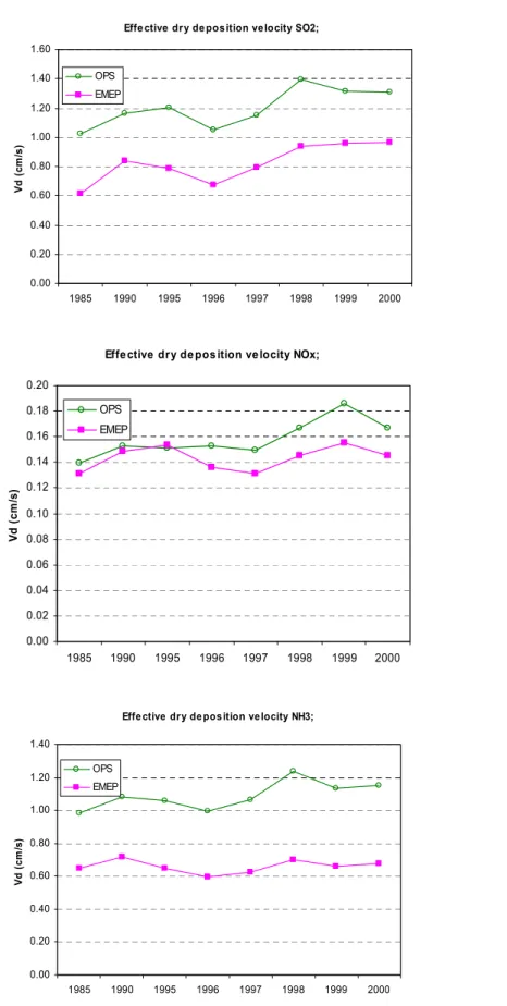
Nowadays dry deposition parameterisations have so many variables that it not easy to see what the relevant differences are. Therefore, as a first comparison, the effective annual average dry deposition velocity is calculated for the EMEP and OPS models. This is done by dividing the total dry deposition flux by the concentration of the primary substance (SO2,
NOx, NH3). This does not exactly provide the dry deposition velocity for the primary
substance, since total dry deposition includes the dry deposition of secondary products. However, in case of the Netherlands, the error made is not large and, moreover, it is for purposes of comparison only. The effective dry deposition velocities are shown for the EMEP and OPS models in Figure 2.2.
The first conclusion is that year-to-year variations are quite similar, probably pointing to meteorological influences being similar in both models. The dry deposition velocities in the OPS model are remarkably higher than in the EMEP model for SO2 and NH3, and
comparable for NOy. To see what causes the difference between the two models it is
necessary to look at the parameters used in both models.
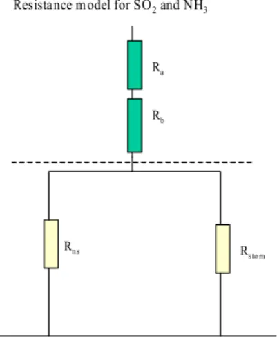
The resistance model for dry deposition of SO2 or NH3 to vegetation, applied in the EMEP
model, is given in Figure 2.1. Common in almost all models are the aerodynamic resistance Ra and the quasi-laminar layer resistance Rb. Especially Ra depends strongly on the roughness
of the surface and is therefore very different for such aspects as forest- and grass-covered surfaces. Dry deposition is assumed to take place along two pathways: via the stomata characterised by Rstom and via other (external or non-stomatal) pathways, here characterised
by a single resistance Rns. Of these two resistances, Rstom is the most elaborated in the
literature and has, most of the time, by far also the highest value of the two. Therefore we concentrate on Rns. This resistance represents the uptake of SO2 and NH3 on the external parts
of the vegetation, e.g., in droplets or water films at the leaf surfaces. It is therefore a function of the chemical composition of the moisture, temperature, air humidity and/or surface wetness.
Rns Rstom
Rb Ra Resistance model for SO2 and NH3
Figure 2.2. Comparison of annual average (for the Netherlands) effective dry deposition velocities for the EMEP and OPS models.
Effe ctive dry de position velocity SO2;
0.00 0.20 0.40 0.60 0.80 1.00 1.20 1.40 1.60 1985 1990 1995 1996 1997 1998 1999 2000 Vd ( cm /s ) OPS EMEP
Effe ctive dry de pos ition ve locity NOx;
0.00 0.02 0.04 0.06 0.08 0.10 0.12 0.14 0.16 0.18 0.20 1985 1990 1995 1996 1997 1998 1999 2000 Vd ( cm /s) OPS EMEP
Effe ctive dry de pos ition ve locity NH3;
0.00 0.20 0.40 0.60 0.80 1.00 1.20 1.40 1985 1990 1995 1996 1997 1998 1999 2000 Vd ( cm /s ) OPS EMEP
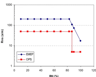
In Figure 2.3 the value of Rns is given as a function of the relative humidity for average
conditions in the Netherlands (molar SO2/NH3 ratio = 0.09, temperature = 9oC). The OPS
model has a lower Rns under all conditions. For wet surfaces the OPS model uses a value of
5 s/m, while the EMEP value has a lower limit of 17 s/m. Assuming that the sum of Ra and
Rb has a value of 50 s/m, Vd has a value of 0.018 m/s for the OPS model and 0.015 for the
EMEP model. In case of a relative humidity of 90% these values are 0.018 and 0.077 s/m, respectively. Except for the dependency on humidity, the approaches differ, also in their dependencies on parameters such as temperature and molar SO2/NH3 ratios. However, the
essential difference between the dry deposition parameterisation in the two models is shown in Figure 2.3; it explains to a large extent why the effective dry deposition velocity in Figure 2.2 (bottom panel) deviates so much between the two models.
Figure 2.3. Comparison of the non-stomatal resistance formulations for NH3.
Figure 2.4. Comparison of the non-stomatal resistance formulations for SO2.
Non-s tom atal re s is tance NH3 vs RH
1 10 100 1000 0 20 40 60 80 100 120 RH (%) Rn s (s /m ) EMEP OPS
Non-stomatal resistance vs relative humidity
1 10 100 1000 0 20 40 60 80 100 120 RH (%) Rn s ( s/ m )
EMEP: dry conditions EMEP:wet conditions OPS: dry conditions OPS: wet conditions
A similar difference between the EMEP and OPS models exists for the non-stomatal resistance of SO2. Here, the EMEP model recognises two conditions: dry and wet, while in
both conditions the resistance varies as a function of the molar SO2/NH3 ratio. The 'dry'
resistance approaches the wet resistance at 100% relative humidity. The DEPAC parameterisation as applied in the OPS model considers a 'wet' condition at a relative humidity of more than 87%. Rns is independent of the SO2/NH3 ratio. In the EMEP model the
'wet' condition exists if there is actual rainfall. The frequency of occurrence of 'wet' is likely to be much higher in the OPS model than in the EMEP model. This leads to lower Rns (on
average) and, consequently, higher dry deposition velocities.
Given the discrepancies and considering the impact of high Vd values on SO2 and NH3
transport and deposition, it is recommended to re-evaluate Rns formulations (especially for
wet conditions) on the basis of original experimental data.
2.2 General comments on dry deposition parameterisations
Dry deposition determines to a large extent the long-range transport capabilities of pollutants and at the same time the atmospheric load of the pollutants to ecosystems. Therefore, source-receptor matrices calculated by long-range transport models are sensitive to the choice of dry deposition parameters (see section 4).
The non-stomatal resistance for ozone is formulated in the EMEP model in a more complex way than for SO2 or NH3. The reason mentioned for this is that the ozone case has been
evaluated more extensively. The resistance model for ozone includes an additional dry deposition pathway, namely via the canopy through the soil or ground cover. One of the variables is the Leaf Area Index, a function of vegetation type. Basically, there is no difference between dry deposition pathways for the various substances. A uniform approach could make parameterisations more transparent, also in terms of the differences between land use types.
The non-stomatal resistance formulation for NH3 in the EMEP model contains dependencies
on temperature, molar SO2/NH3 ratios and humidity. One should expect similar dependencies
for SO2 and other soluble gases because the same processes and the same interaction are
concerned. In the EMEP model the formulation for SO2 is much simpler, while probably
much more literature data is available. When it comes to non-linearity issues, the dry deposition dependency between NH3 and SO2 may play an important role in future.
The non-stomatal resistance formulation for NH3 in the EMEP model describes more or less
the expected dependencies on parameters such as temperature, humidity and the pollution climate. All these parameters are theoretically defendable and to some extent observed in the laboratory. However, current field experiments are not distinctive enough to positively support a reliable quantification of the necessary parameters.
3. EMEP versus OPS on a 50 x 50 km grid
The grid size of the EMEP model has decreased from about 150 x 150 km to a current resolution of about 50 x 50 km (the EMEP grid cells are exactly 50 x 50 km but only at 60ºN). The EMEP observational network used to validate the model are located far apart on background sites in Europe. These observations alone might not be sufficient to validate the variability of the EMEP model on the 50 x 50 km grid scale. To test the performance of the EMEP model on the 50 x 50 km grid, we compared its results with output from the OPS model (Van Jaarsveld, 1995) for yearly average concentrations of SO2, NOx, and NH3, as
well as dry and wet depositions of oxidised sulphur, oxidised nitrogen and reduced nitrogen for the Netherlands for 1985, 1990 and 1995-2000. The EMEP results are also compared with observations for the Netherlands.
In the Netherlands the OPS model is used for the calculation concentrations and deposition of acidifying compounds. By combining a Gaussian plume model for local transport using a trajectory model for the long-range transport, the model is capable of calculating the effects of very local emission sources (< 100 m), as well as contributions from foreign sources, for example. The model has been validated by comparing SO2, NOx and NH3 concentrations and
depositions with measurements from the RIVM’s Netherlands air quality monitoring network (LML) (Elzakker, 2001).
To compare the OPS model results (RIVM, 2003) with the EMEP model results, the OPS model results on a 5 x 5 km grid resolution were converted to the EMEP grid format on a 50 x 50 km resolution. The conversion was done as follows: the average of all the OPS grid cells was taken for each EMEP grid cell. Of the cell centres lying in the EMEP grid cell, only cells of which more than 45% of the area of the EMEP grid cell occurred within the OPS area were considered for the comparison; the average and standard deviation in the OPS results was calculated. Background values were added to the dry and wet depositions calculated by the OPS model to account for emissions from outside Europe and the North Sea. The background values for the dry and wet deposition of oxidised sulphur were 38 and 134 mg S/m2, respectively. For the dry and wet deposition of oxidised nitrogen, these were 18 and 50 mg N/m2, respectively, and for the dry and wet deposition of reduced nitrogen, 67 and 38 mg N/m2, respectively.
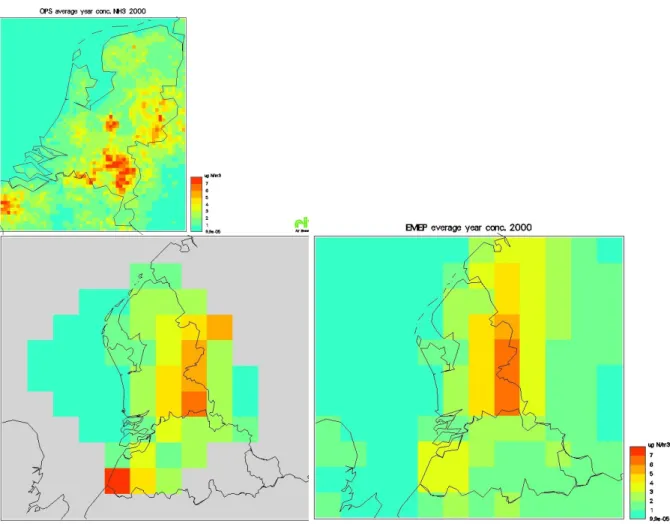
As an example of the conversion, the concentrations of NH3 in air are shown in Figure 3.1.
The top panel in Figure 3.1 shows the NH3 concentration on the OPS grid of 5 x 5 km and the
bottom left panel shows the OPS concentration on the EMEP grid of 50 x 50 km. For comparison, the bottom right panel of Figure 3.1 shows the NH3 concentrations of the EMEP
model.
In Figure 3.2, the concentrations and depositions calculated with the OPS model are compared with those of the EMEP model per grid cell for the year 2000, being representative of all years between1985-2000 with respect to the correlation and the slope of the least-squares fit of the correlation’s. In general, there is a large dispersion in the converted OPS results for each EMEP grid cell, especially at high concentrations (Figure 3.2). For SO2 and
NH3, the EMEP and OPS concentrations agree quite well, the EMEP concentrations are
slightly higher for most grid cells. For NOx, the OPS model calculates much higher
concentrations for each cell than the EMEP model, almost a factor of two. This underestimation of the NOx concentration in the EMEP model might be related to the fact
that Eulerian (grid) models often have difficulties with the large spatial gradients in NOx
close to emission sources. After being emitted, NOx is distributed over the whole grid cell,
The dry deposition (Figure 3.2) calculated by the EMEP model is much lower than that calculated by the OPS model for oxidised and reduced nitrogen. For most grid cells, the dry deposition of the EMEP model is, for oxidised sulphur, lower than that of the OPS model, but for low OPS values, both agree quite well. The wet deposition calculated by the EMEP model is always much higher than in the OPS model for all three components.
In Tables 3.1 to 3.4 and Figures 3.3 to 3.6 the averaged concentrations and depositions of the EMEP model are compared with those of the OPS model and with measurements. For comparing the averaged concentrations and depositions the data are averaged over the area of the Netherlands. The average values are calculated using a weighted mean of the fraction of the EMEP cell covering the Netherlands. The measurements are taken from the RIVM’s Netherlands air quality monitoring network (LML) (Elzakker, 2001).
Figure 3.1. Air concentration of NH3 (in µg m-3) in the Netherlands from the OPS model (top
panel), from the OPS model converted to the EMEP grid (bottom left panel), and from the EMEP model (bottom right panel).
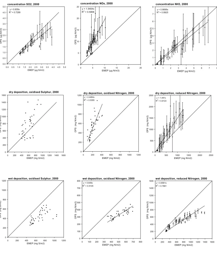
Figure 3.2. Correlation between the EMEP and OPS results for the concentrations in air of
SO2, NOx and NH3 and the dry and wet deposition of oxidised sulphur (SOx) along with
oxidised (NOy) and reduced (NHx) nitrogen in the Netherlands for 2000. The OPS results
were converted to the EMEP grid. The vertical bars represent the variability (standard deviation) in the OPS grid cells.
dry deposition, oxidised Nitrogen, 2000
y = 2.4464x R2 = 0.5355 0 200 400 600 800 1000 1200 0 200 400 600 800 1000 1200 EMEP (mg N/m2) O PS ( m g N /m 2)
dry deposition, oxidised Sulphur, 2000
0 200 400 600 800 1000 1200 1400 1600 0 200 400 600 800 1000 1200 1400 1600 EMEP (mg S/m2) OP S (m g S /m 2)
dry deposition, reduced Nitrogen, 2000
y = 1.491x R2 = 0.8123 0 500 1000 1500 2000 2500 0 500 1000 1500 2000 2500 EMEP (mg N/m2) O PS (m g N /m 2)
wet deposition, oxidised Sulphur, 2000
0 200 400 600 800 1000 1200 0 200 400 600 800 1000 1200 EMEP (mg S/m2) OP S (m g S /m 2)
wet deposition, oxidised Nitrogen, 2000
y = 0.649x R2 = 0.5105 0 100 200 300 400 500 600 700 800 0 100 200 300 400 500 600 700 800 EMEP (mg N/m2) OP S (m g N /m 2 )
wet deposition, reduced Nitrogen, 2000
y = 0.6561x R2 = 0.7881 0 200 400 600 800 1000 1200 1400 1600 0 200 400 600 800 1000 1200 1400 1600 EMEP (mg N/m2) OP S ( m g N /m 2 ) concentration SO2, 2000 y = 0.835x R2 = 0.7299 0.0 0.5 1.0 1.5 2.0 2.5 3.0 3.5 4.0 4.5 5.0 0.0 0.5 1.0 1.5 2.0 2.5 3.0 3.5 4.0 4.5 5.0 EMEP (µg S/m3) O PS ( µ g S /m 3) concentration NOx, 2000 y = 1.9404x R2 = 0.5856 0 5 10 15 20 25 0 5 10 15 20 25 EMEP (µg N/m3) OP S ( µ g N /m 3 ) concentration NH3, 2000 y = 0.8688x R2 = 0.8925 0 1 2 3 4 5 6 7 8 0 1 2 3 4 5 6 7 8 EMEP (µg N/m3) OP S ( µ g N /m 3 )
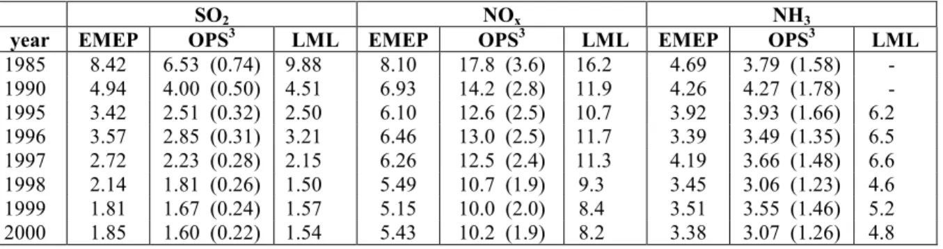
Table 3.1. Concentration of SO2 (µg S m ), NOx and NH3 (µg N m ) in the Netherlands from
the OPS model, the Eulerian EMEP model and LML observations2.
SO2 NOx NH3
year EMEP OPS3 LML EMEP OPS3 LML EMEP OPS3 LML
1985 8.42 6.53 (0.74) 9.88 8.10 17.8 (3.6) 16.2 4.69 3.79 (1.58) -1990 4.94 4.00 (0.50) 4.51 6.93 14.2 (2.8) 11.9 4.26 4.27 (1.78) -1995 3.42 2.51 (0.32) 2.50 6.10 12.6 (2.5) 10.7 3.92 3.93 (1.66) 6.2 1996 3.57 2.85 (0.31) 3.21 6.46 13.0 (2.5) 11.7 3.39 3.49 (1.35) 6.5 1997 2.72 2.23 (0.28) 2.15 6.26 12.5 (2.4) 11.3 4.19 3.66 (1.48) 6.6 1998 2.14 1.81 (0.26) 1.50 5.49 10.7 (1.9) 9.3 3.45 3.06 (1.23) 4.6 1999 1.81 1.67 (0.24) 1.57 5.15 10.0 (2.0) 8.4 3.51 3.55 (1.46) 5.2 2000 1.85 1.60 (0.22) 1.54 5.43 10.2 (1.9) 8.2 3.38 3.07 (1.26) 4.8
Table 3.2. Dry deposition1 of oxidised sulphur (mg S m-2) and oxidised and reduced nitrogen
(mg N m-2) in the Netherlands from the OPS model and the Eulerian EMEP model.
oxidised Sulphur, SOx oxidised Nitrogen, NOy reduced Nitrogen, NHx
year EMEP OPS3 LML EMEP OPS3 LML EMEP OPS3 LML
1985 1635 2113 (799) - 334 784 (143) - 955 1177 (365) -1990 1313 1465 (618) - 325 684 (120) - 961 1459 (451) -1995 852 953 (373) - 295 599 (108) - 799 1315 (415) -1996 760 947 (349) - 278 627 (113) - 634 1098 (333) -1997 679 808 (303) - 259 589 (105) - 824 1228 (381) -1998 633 796 (317) - 251 564 (100) - 760 1195 (377) -1999 546 693 (272) - 252 586 (106) - 732 1269 (405) -2000 563 661 (253) - 248 536 ( 95) - 723 1113 (357)
-Table 3.3. Wet deposition1 of oxidised sulphur (mg S m-2) and oxidised and reduced nitrogen
(mg N m-2) in the Netherlands from the OPS model, the Eulerian EMEP model and LML
observations1.
oxidised Sulphur, SOx oxidised Nitrogen, NOy reduced Nitrogen, NHx
year EMEP OPS3 LML EMEP OPS3 LML EMEP OPS3 LML
1985 2095 1159 (85) 1069 754 517 (16) 498 1048 736 (72) 990 1990 1275 887 (63) 982 537 427 (12) 428 717 627 (70) 934 1995 863 660 (43) 701 473 393 (11) 412 643 482 (54) 846 1996 738 533 (33) 579 466 340 ( 7) 364 615 411 (39) 783 1997 643 535 (38) 608 473 334 ( 7) 363 688 466 (46) 846 1998 886 683 (55) 816 640 424 (11) 511 907 590 (62) 1021 1999 664 577 (44) 643 501 431 (13) 449 737 525 (52) 864 2000 680 573 (43) 682 533 386 (11) 518 789 515 (50) 939
Table 3.4. Total (dry + wet) deposition1 of oxidised sulphur (mg S m-2) and oxidised and
reduced nitrogen (mg N m-2) in the Netherlands from the OPS model and the Eulerian EMEP
model.
oxidised Sulphur, SOx oxidised Nitrogen, NOy reduced Nitrogen, NHx
year EMEP OPS LML EMEP OPS LML EMEP OPS LML
1985 3730 3273 - 1088 1302 - 2003 1913 -1990 2588 2353 - 862 1112 - 1678 2086 -1995 1715 1614 - 768 993 - 1442 1797 -1996 1498 1481 - 744 968 - 1249 1509 -1997 1322 1344 - 732 924 - 1512 1694 -1998 1519 1480 - 891 989 - 1667 1785 -1999 1210 1271 - 753 1018 - 1469 1794 -2000 1243 1235 - 781 923 - 1512 1628
-1) Values are averaged over the area of the Netherlands using the EMEP grid.
2) Observations from the LML network (Elzakker, 2001) represent the average for the area of the Netherlands. 3) The average variability (standard deviation of the average) in the OPS grid cells mapped onto the EMEP grid is given in parentheses.
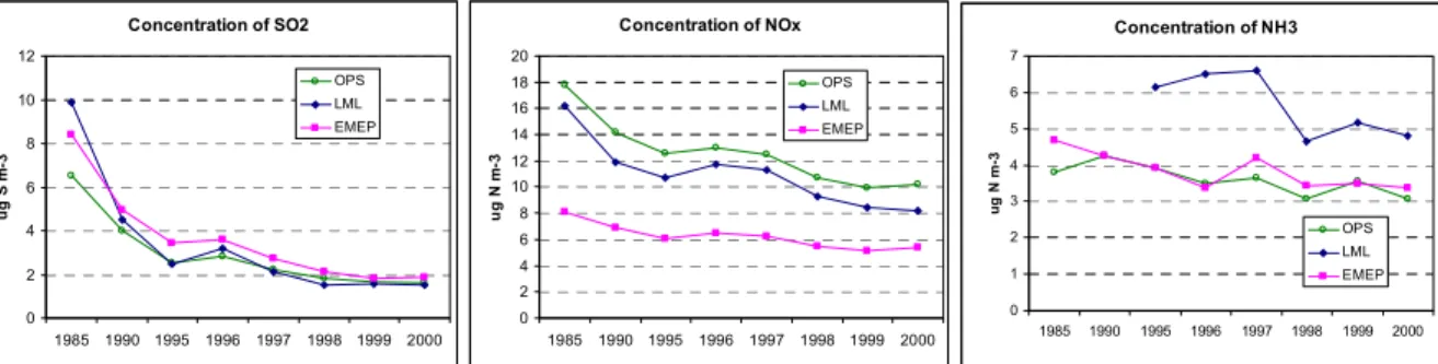
Concentration of SO2 0 2 4 6 8 10 12 1985 1990 1995 1996 1997 1998 1999 2000 ug S m -3 OPS LML EMEP Concentration of NOx 0 2 4 6 8 10 12 14 16 18 20 1985 1990 1995 1996 1997 1998 1999 2000 ug N m -3 OPS LML EMEP Concentration of NH3 0 1 2 3 4 5 6 7 1985 1990 1995 1996 1997 1998 1999 2000 ug N m -3 OPS LML EMEP
Figure 3.3. Comparison of the concentrations in air of SO2, NOx and NH3 in the Netherlands
for the EMEP and OPS models and the LML measurements.
Dry deposition of oxidised Sulphur
0 500 1000 1500 2000 2500 1985 1990 1995 1996 1997 1998 1999 2000 mg S m -2 OPS EMEP
Dry deposition of oxidised Nitrogen
0 100 200 300 400 500 600 700 800 900 1985 1990 1995 1996 1997 1998 1999 2000 mg N m -2 OPS EMEP
Dry deposition of reduced Nitrogen
0 200 400 600 800 1000 1200 1400 1600 1985 1990 1995 1996 1997 1998 1999 2000 mg N m-2 OPS EMEP
Figure 3.4. Comparison of the dry deposition of oxidised sulphur and oxidised and reduced nitrogen in the Netherlands for the EMEP and OPS models.
Wet deposition of oxidised Sulphur
0 500 1000 1500 2000 2500 1985 1990 1995 1996 1997 1998 1999 2000 mg S m-2 OPS LML EMEP
Wet deposition of oxidised Nitrogen
0 100 200 300 400 500 600 700 800 1985 1990 1995 1996 1997 1998 1999 2000 mg N m -2 OPS LML EMEP
Wet deposition of reduced Nitrogen
0 200 400 600 800 1000 1200 1985 1990 1995 1996 1997 1998 1999 2000 mg N m-2 OPS LML EMEP
Figure 3.5. Comparison of the wet deposition of oxidised sulphur and oxidised and reduced nitrogen in the Netherlands for the EMEP and OPS models and the LML measurements.
Total deposition of oxidised Sulphur
0 500 1000 1500 2000 2500 3000 3500 4000 1985 1990 1995 1996 1997 1998 1999 2000 mg S m-2 OPS EMEP
Total deposition of oxidised Nitrogen
0 200 400 600 800 1000 1200 1400 1985 1990 1995 1996 1997 1998 1999 2000 mg N m-2 OPS EMEP
Total deposition of reduced Nitrogen
0 500 1000 1500 2000 2500 1985 1990 1995 1996 1997 1998 1999 2000 mg N m-2 OPS EMEP
Figure 3.6. Comparison of the total (dry + wet) deposition of oxidised sulphur and oxidised and reduced nitrogen in the Netherlands for the EMEP and OPS models.
Comparing the yearly averaged SO2 concentration in the Netherlands (Table 3.1 and
Figure 3.3, we found that concentrations calculated with the EMEP model for the later years were close to the OPS results and the measurements. The EMEP values are always slightly higher than the OPS results and the measurements, except for 1985 when the EMEP model yielded values about 15% below the measurements. The NOx concentrations calculated with
the EMEP model are about 50% lower than the OPS concentrations and about 40% lower than the measured concentrations for all the years. This underestimation of the NOx
concentrations by the EMEP model, compared with the measurements, is in agreement with the EMEP report (Simpson et al., 2003). They find a somewhat smaller underestimation by considering two stations (Kollumerwaard and Vredepeel) with for Dutch standards low NOx
concentrations. For the NH3 concentrations, the EMEP results are close to the OPS results,
but both are 30 to 40% lower than the measured concentrations. This occurrence, in combination with the fact that both models underestimate the wet deposition of NHx,
confirms the existence of the so-called ‘ammonia gap’ (Van Jaarsveld and Van Pul, 2002). The dry deposition calculated with the EMEP model is lower than that calculated with the OPS model for all compounds, while the wet deposition is always higher. Consequently, the total (dry + wet) deposition of both models are similar, especially for oxidised sulphur. The dry deposition of the EMEP model is lower than the OPS model, by an average of about 15%, 55%, and 35%, for oxidised sulphur, oxidised nitrogen, and reduced nitrogen, respectively. There are no measurements to compare these dry depositions with. The dry deposition is determined by the concentration in the air and the dry deposition velocity (see section 4.1). Using a larger dry deposition, velocity will almost proportionally increase the dry deposition, but result in a (small) decrease in the atmospheric concentration. Due to conservation of mass, the wet deposition decreases if the dry deposition increases, resulting in only a small change in the total deposition.
The wet deposition calculated with the EMEP model is higher for all compounds (about 20-50%) than that calculated with the OPS model. The differences between the EMEP and OPS models for the wet deposition of oxidised sulphur decreased from 81% in 1985 to 19% in 2000. Especially for the later years, there is a good agreement with the measurements. The wet deposition of oxidised and reduced nitrogen of the EMEP model is about 25% higher and about 20% lower, respectively, than the measurements.
The standard deviation around the average values in the OPS grid cells is shown in Figure 3.2 and Tables 3.1 to 3.3 to express the fact that the concentrations and depositions of the OPS grid cells on a 5 x 5 km grid scale exhibit considerable variation. Closer investigation of this variability shows that it is about a constant percentage of the average value and that there is no trend over the years in this variability. For example, the standard deviation of the OPS grid cells for the SO2 concentration in air is on average about 12% for all years.
4.
Source-receptor relationships for the Netherlands
The OPS model (Van Jaarsveld, 1995) is used at RIVM-MNP to calculate source-receptor relationships for NOx, SOx and NHx deposition. A full evaluation of the source-receptorrelationship for Europe requires a large number of scenario calculations with a European model due to the non-linearity of the processes involved. This is outside the scope of this analysis and of the current version of the OPS model. This chapter compares the contribution of countries to the deposition in the Netherlands, as calculated by the EMEP and OPS models. For this purpose the year 2000 is selected. The EMEP data is taken from the EMEP Status Report 1/2003 Part III (Tarrasón et al., 2003) and the OPS data from the calculations carried out in the framework of the Netherlands Environmental Balance 2003 (RIVM, 2003). The OPS data are calculated on the basis of the same national emission totals as used in the EMEP model; however, the spatial distribution was not the same nor were the physical properties of the emission sources (release height, heat content, spatial resolution). The spatial resolution for emissions in the Netherlands, Belgium and Germany was 5 x 5 km, while large point source emissions were treated as point sources conforming with their exact locations. Separate 5 x 5 km distributions were used for the remaining (non-point source) emissions, segregated into specific categories (industrial, mobile sources, inland shipping, agricultural sources etc.).
The comparison is based on the sum of the deposition on the Netherlands territory. Because the area considered in the two models is not the same surface area (OPS: 34958 km2, EMEP: 42485 km2), the OPS data will be systematically lower than the EMEP data. However, a simple scaling on the basis of the respective surface areas would lead to an overestimation, because the EMEP area includes more of the surrounding waters where deposition is lower than on the land area. In order to be compatible with the comparison in section 3, we have not applied a correction factor. The comparison on the total deposition may therefore differ from what is given in section 3. Results are given in Table 4.2 and Figure 4.1
One difference in approach between the EMEP and the OPS models is that the Eulerian EMEP model applies a much larger Boundary Initial Conditions (BIC) at the model domain boundaries than the OPS model. One can consider them as background concentrations accounting for trans-Atlantic transport, for example. The initial concentrations represent, in fact, a source term and signify a certain contribution to the Netherlands. A similar problem applies to the OPS model. Since only anthropogenic emissions in Europe are considered and no shipping emissions are taken into account (except North Sea emissions), background contributions are added to the model results. These depositions are based on estimates made by Locht and Van Aalst (1988). Table 4.1 provides the values for the different compounds.
Table 4.1. Background depositions applied to the Netherlands.
Unit dry wet total
NOy mg N m-2 a-1 18 50 69
NHx mg N m-2 a-1 67 38 105
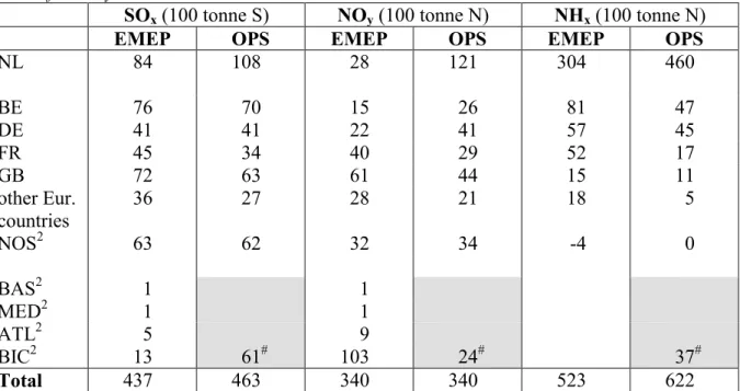
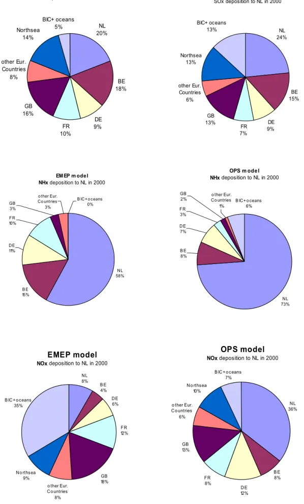
Table 4.2. Deposition contributions to the Netherlands according to the EMEP and the OPS models for the year 2000.
SOx (100 tonne S) NOy (100 tonne N) NHx (100 tonne N)
EMEP OPS EMEP OPS EMEP OPS
NL 84 108 28 121 304 460 BE 76 70 15 26 81 47 DE 41 41 22 41 57 45 FR 45 34 40 29 52 17 GB 72 63 61 44 15 11 other Eur. countries 36 27 28 21 18 5 NOS2 63 62 32 34 -4 0 BAS2 1 1 MED2 1 1 ATL2 5 9 BIC2 13 61# 103 24# 37# Total 437 463 340 340 523 622
1) The grid and total area used in the EMEP model differs here from the area used in the OPS model, which gives a difference in the absolute values between the models. Furthermore, figures in this table can not be directly compared with those in section 3 (Figure 3.6 and Table 3.4).
2) NOS = North Sea; BAS = Baltic Sea; MED = Mediterranean; ATL = Atlantic; BIC = Boundary and Initial Conditions
#) Background value, accounting for non-European and natural source contributions (see section 3).
The following observations can be made with respect to the source-receptor matrices (Table 4.2 and Figure 4.1):
• The source-receptor matrices for SOx calculated by the two models are in good
agreement.
• The agreement for reduced nitrogen is reasonable. The EMEP model calculates larger contributions from Belgium and Germany and a lower contribution from the Netherlands. • The relative contribution from the Netherlands to the Netherlands is always higher in the
OPS model than in the EMEP model: for SOx EMEP is 20% and OPS: 24%), for NHx,
EMEP is 58% and OPS 73% and for NOy EMEP is 8% and OPS 36%). This is in line
with the findings in chapter 3 that the OPS model calculates higher concentrations (NOx)
and/or uses higher dry deposition velocities (SO2 and NH3; see also chapter 2, Figure
2.1).
• The largest discrepancies are found for oxidised nitrogen. Here, the local deposition contribution of Dutch emissions to the Netherlands is a factor of 4 higher than in the EMEP model. The Dutch emissions contribute only 8% to the emissions in the Netherlands. This was 30-35% in the pervious version of the Eulerian model and 15-20% in the Lagrangian model (EMEP, 2001). The NOy contributions from Belgium and
Germany are now also much lower in the EMEP model than in the OPS model. A comparison of model results with observations in the Netherlands (chapter 3) illustrates that the EMEP model strongly underestimates NOx concentrations and dry deposition,
while the wet deposition is overestimated. This is not related to the combination of low sources and a low vertical resolution of the model, as can be seen in the case of NH3
• Another striking difference is the influence of BIC for oxidised nitrogen. The EMEP model suggests that almost 30% of the deposition is due to sources outside Europe. In the previous version of the EMEP Eulerian model, this BIC term contributed only 3-5% to the deposition of NOy in the Netherlands. Apparently, the EMEP model has difficulties
modelling oxidised nitrogen.
• The EMEP model reports no contributions of BIC for NHx. It is unclear if these are either
not taken into account or are not significant.
At the TFMM workshop in Oslo in November 2003 the data of Table 4.2 was discussed with EMEP. They explained that the SRMs calculated by the EMEP UNIFIED model (EMEP Status Report 1/2003 Part III, Tarrasón et al., 2003) are not the final results. They explained that the large BIC term for NOy is not a true boundary condition, but comes from the way the
SRMs for NOy are calculated. They are still working on the SRM calculations and expect to
Figure 4.1. Deposition contributions to the Netherlands according to the EMEP and OPS models for the year 2000.
SOx deposition to NL in 2000 NL 20% BE 18% DE 9% FR 10% GB 16% other Eur. Countries 8% Northsea 14% BIC+ oceans 5% OPS SOx deposition to NL in 2000 NL 24% BE 15% DE 9% FR 7% GB 13% other Eur. Countries 6% Northsea 13% BIC+ oceans 13% EM EP m ode l NHx deposition to NL in 2000 NL 58% B E 15% B IC+ o ceans 0% FR 10% DE 11% o ther Eur. Co untries 3% GB 3% OPS model NOx deposition to NL in 2000 NL 36% No rthsea 10% B IC+ o ceans 7% o ther Eur. Co untries 6% FR 8% DE 12% GB 13% B E 8% OPS m odel NHx deposition to NL in 2000 NL 73% B IC+ o ceans 6% o ther Eur. Co untries 1% FR 3% D E 7% GB 2% B E 8% EMEP model NOx deposition to NL in 2000 NL 8% B E 4% No rthsea 9% GB 18% o ther Eur. Co untries 8% DE 6% FR 12% B IC+ o ceans 35%
5. Distribution of emissions
In Task I of the evaluation EMEP compared the model results with measurements for 1980-2000. This comparison depends strongly on the emissions and their geographical distribution as used in the EMEP model. Countries were requested to report their emissions and the geographical distribution of the emissions to EMEP. We have compared the geographical distributions of the EMEP’s SOx and NOx emissions on the 50 x 50 km grid for selected
countries, i.e., Germany, The Netherlands and Poland and selected years, 1980 and from 1985-2000. In Germany and Poland significant changes in the geographical distribution of the SOx and NOx emissions from 1980 to 2000 are be expected as a result of changes in the
economies of these countries. Investigated were the low and high emission categories and the emissions per sector.
Tables 5.1 and 5.2 show the SOx and NOx emissions for the low and high emission
categories, as obtained from the EMEP website (Webdab, 2002). The ratios between the emissions in both categories are shown as the percentage emitted per grid cell (compared with the total emission in the country). It can be seen that:
1. the ratio between the emissions in the high and low emission categories is, per grid cell, the same for all the years in the period 1980-2000 (i.e., 1980, 1985-2000). This holds for all grid cells in the three selected countries and for both the SOx and NOx emissions.
2. the geographical distribution of the SOx and NOx emissions (low and high emission
categories) in the selected countries is identical for all of 1980 and 1985-2000, i.e. the same fraction of the total emissions in a country is emitted in the grid cells for all years. 3. the ratio between emissions in the high and low emission categories for Poland is the
same for all cells and all years.
The EMEP emissions are also subdivided in 11 sectors, e.g. combustion, transport, etc. The percentage of the emissions in the grid cells, compared with the total emission in the country, is analysed for Germany, The Netherlands and Poland for the years 1980 and 1985-2000. The data for Germany are shown in Table 5.3 for the three sectors with the largest emissions and for the years 1980 and 2000. From this table it can be seen that:
4. the geographical distribution of the SOx and NOx emissions of all sectors in the selected
countries does not change through the years 1980-2000, i.e. the same fraction of the total emissions of a sector in a country is emitted in the grid cells for all years.
The absence of changes in geographical distribution in the EMEP emissions from 1980 to 2000 will likely affect the comparison between modelled and measured concentrations. This will hold especially for Eastern Europe, where large changes in emissions and their geographical distributions are expected due to the changes in their economies since the 1980s. The effects for Western Europe will probably be much smaller.
The emissions discussed here are obtained from the EMEP website (Webdab, 2002). By the end of October 2003 EMEP released the new version of the emission database, Webdab 2003. An analysis of the new emissions showed that, although some numbers have changed, the conclusions about the constant geographical distributions, are still valid. The emissions show changes in geographical distributions only for the years 2000 and 2001.
In a discussion, after this report was placed on the EMEP website, EMEP explained that the low and high emissions of Webdab 2002 have not been used for the Unified model. They also explained that, although countries are requested to report geographical distributions of their emissions, many don't send this information to EMEP and EMEP uses what is available.
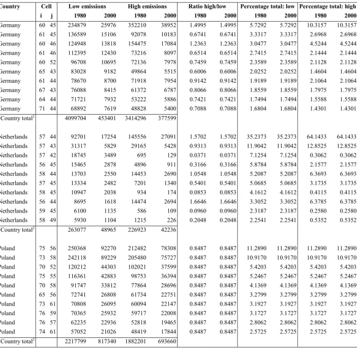
Table 5.1. Geographical distribution of SOx emissions on the EMEP 50 x 50 km grid for
Germany, The Netherlands and Poland for 1980 and 2000, showing the emissions (in Mg
SO2) in the low and high emission categories for the grid cells with the largest emissions (in
1980), and the ratio between the high and low emission categories and the percentage of the
emissions in the grid cells compared with the total emission in the country1.
Country Cell Low emissions High emissions Ratio high/low Percentage total: low Percentage total: high
i j 1980 2000 1980 2000 1980 2000 1980 2000 1980 2000 Germany 60 45 234879 25976 352210 38952 1.4995 1.4995 5.7292 5.7292 10.3157 10.3157 Germany 61 45 136589 15106 92078 10183 0.6741 0.6741 3.3317 3.3317 2.6968 2.6968 Germany 60 46 124948 13818 154475 17084 1.2363 1.2363 3.0477 3.0477 4.5244 4.5244 Germany 61 46 112395 12430 73216 8097 0.6514 0.6514 2.7415 2.7415 2.1444 2.1444 Germany 60 52 96708 10695 72136 7978 0.7459 0.7459 2.3589 2.3589 2.1128 2.1128 Germany 65 43 83028 9182 49864 5515 0.6006 0.6006 2.0252 2.0252 1.4604 1.4604 Germany 61 44 78670 8700 71918 7954 0.9142 0.9142 1.9189 1.9189 2.1064 2.1064 Germany 67 43 76088 8415 61372 6787 0.8066 0.8066 1.8559 1.8559 1.7975 1.7975 Germany 64 44 71721 7932 53222 5886 0.7421 0.7421 1.7494 1.7494 1.5588 1.5588 Germany 71 44 68892 7619 48828 5400 0.7088 0.7088 1.6804 1.6804 1.4301 1.4301 Country total2 4099704 453401 3414296 377599 Netherlands 57 44 92701 17254 145556 27091 1.5702 1.5702 35.2373 35.2373 64.1433 64.1433 Netherlands 57 43 31317 5829 29165 5428 0.9313 0.9313 11.9042 11.9042 12.8525 12.8525 Netherlands 57 42 18745 3489 695 129 0.0371 0.0371 7.1254 7.1254 0.3062 0.3062 Netherlands 56 45 15465 2878 4896 911 0.3166 0.3166 5.8784 5.8784 2.1577 2.1577 Netherlands 58 44 13703 2550 14453 2690 1.0548 1.0548 5.2087 5.2087 6.3693 6.3693 Netherlands 57 45 13334 2482 7201 1340 0.5401 0.5401 5.0685 5.0685 3.1735 3.1735 Netherlands 58 45 10947 2038 934 174 0.0853 0.0853 4.1612 4.1612 0.4115 0.4115 Netherlands 56 44 8695 1618 14474 2694 1.6646 1.6646 3.3052 3.3052 6.3785 6.3785 Netherlands 59 45 6100 1135 586 109 0.0960 0.0960 2.3187 2.3187 0.2580 0.2580 Netherlands 58 49 5930 1104 1215 226 0.2048 0.2048 2.2541 2.2541 0.5352 0.5352 Country total2 263077 48965 226923 42236 Poland 75 56 250368 92270 212482 78308 0.8487 0.8487 11.2890 11.2890 11.2890 11.2890 Poland 73 58 242118 89229 205480 75727 0.8487 0.8487 10.9170 10.9170 10.9170 10.9170 Poland 70 52 120212 44303 102021 37599 0.8487 0.8487 5.4203 5.4203 5.4203 5.4203 Poland 75 55 116361 42883 98753 36394 0.8487 0.8487 5.2467 5.2467 5.2467 5.2467 Poland 70 58 91747 33812 77864 28696 0.8487 0.8487 4.1369 4.1369 4.1369 4.1369 Poland 65 56 72741 26808 61734 22751 0.8487 0.8487 3.2799 3.2799 3.2799 3.2799 Poland 73 61 70808 26095 60094 22147 0.8487 0.8487 3.1927 3.1927 3.1927 3.1927 Poland 76 59 70365 25932 59717 22008 0.8487 0.8487 3.1727 3.1727 3.1727 3.1727 Poland 76 57 62235 22936 52818 19465 0.8487 0.8487 2.8062 2.8062 2.8062 2.8062 Poland 74 61 57052 21026 48419 17844 0.8487 0.8487 2.5725 2.5725 2.5725 2.5725 Country total2 2217799 817340 1882201 693660
1) The data of only a few grid cells per country and two years are shown, but the same results can be seen for all grid cells and all the years in 1980 and 1985-2000.
Table 5.2. Geographical distribution of NOx emissions on the EMEP 50 x 50 km grid for
Germany, The Netherlands, and Poland for 1980 and 2000. Shown are the emissions (in Mg
NO2) in the low and high emission categories for the grid cells with the largest emissions (in
1980), as well as the ratio between the high and low emission categories and the percentage
of the emissions in the grid cells compared with the total emission in the country1.
Country Cell Low emissions High emissions Ratio high/low Percentage total: low Percentage total: high
i j 1980 2000 1980 2000 1980 2000 1980 2000 1980 2000 Germany 60 45 85061 41765 36342 17844 0.4272 0.4272 2.9679 2.9679 7.7657 7.7657 Germany 61 45 65450 32136 12979 6373 0.1983 0.1983 2.2837 2.2837 2.7734 2.7734 Germany 61 46 55497 27249 10562 5186 0.1903 0.1903 1.9364 1.9364 2.2570 2.2570 Germany 64 44 49668 24387 7246 3558 0.1459 0.1459 1.7330 1.7330 1.5483 1.5483 Germany 67 43 48680 23902 8949 4394 0.1838 0.1838 1.6985 1.6985 1.9123 1.9123 Germany 60 46 47831 23485 19175 9415 0.4009 0.4009 1.6689 1.6689 4.0975 4.0975 Germany 61 44 44506 21852 9987 4903 0.2244 0.2244 1.5529 1.5529 2.1340 2.1340 Germany 71 44 44408 21805 7068 3470 0.1592 0.1592 1.5495 1.5495 1.5103 1.5103 Germany 60 52 43159 21191 9891 4856 0.2292 0.2292 1.5059 1.5059 2.1135 2.1135 Germany 64 45 42958 21093 5840 2868 0.1360 0.1360 1.4989 1.4989 1.2480 1.2480 Country total2 2866019 1407221 467981 229779 Netherlands 57 44 91297 65925 18364 13261 0.2011 0.2011 17.9905 17.9905 24.3146 24.3146 Netherlands 57 45 61268 44241 7660 5531 0.1250 0.1250 12.0731 12.0731 10.1417 10.1417 Netherlands 58 45 48299 34877 1973 1425 0.0409 0.0409 9.5176 9.5176 2.6128 2.6128 Netherlands 58 44 39378 28434 7100 5127 0.1803 0.1803 7.7596 7.7596 9.4005 9.4005 Netherlands 59 45 23816 17197 1240 896 0.0521 0.0521 4.6930 4.6930 1.6422 1.6422 Netherlands 57 43 23573 17022 5675 4098 0.2407 0.2407 4.6451 4.6451 7.5139 7.5139 Netherlands 59 44 21094 15232 1442 1041 0.0683 0.0683 4.1568 4.1568 1.9087 1.9087 Netherlands 58 46 20664 14921 908 656 0.0439 0.0439 4.0719 4.0719 1.2022 1.2022 Netherlands 57 42 16761 12103 2000 1444 0.1193 0.1193 3.3029 3.3029 2.6479 2.6479 Netherlands 59 46 15229 10997 876 633 0.0575 0.0575 3.0010 3.0010 1.1600 1.1600 Country total2 507473 366442 75527 54538 Poland 75 56 77320 52721 27588 18811 0.3568 0.3568 8.5360 8.5360 8.5360 8.5360 Poland 73 58 55330 37727 19742 13461 0.3568 0.3568 6.1083 6.1083 6.1083 6.1083 Poland 75 55 51805 35324 18484 12603 0.3568 0.3568 5.7192 5.7192 5.7192 5.7192 Poland 76 57 41156 28062 14684 10013 0.3568 0.3568 4.5436 4.5436 4.5436 4.5436 Poland 73 61 38807 26461 13846 9441 0.3568 0.3568 4.2843 4.2843 4.2843 4.2843 Poland 74 55 23325 15904 8322 5675 0.3568 0.3568 2.5751 2.5751 2.5751 2.5751 Poland 65 56 22067 15046 7873 5368 0.3568 0.3568 2.4361 2.4361 2.4361 2.4361 Poland 70 58 19653 13401 7012 4781 0.3568 0.3568 2.1697 2.1697 2.1697 2.1697 Poland 74 61 18811 12827 6712 4577 0.3568 0.3568 2.0768 2.0768 2.0768 2.0768 Poland 72 59 15300 10432 5459 3722 0.3568 0.3568 1.6891 1.6891 1.6891 1.6891 Country total2 905808 617630 323192 220370
1) The data of only a few grid cells per country and two years are shown, but the same results can be seen for all grid cells and all of 1980 and 1985-2000.
Table 5.3. Geographical distribution of SOx emissions on the EMEP 50 x 50 km grid for the
three largest emissions sectors for Germany for 1980 and 2000. Shown are the emissions (in
Mg SO2) for the grid cells with the largest emissions (in 1980, as well as the percentage of
the emissions in the grid cells compared with the total emission in the country1.
Cell Emissions in 1980 Emissions in 2000 Percentage of country total i j 1 Energy industries 2 Non-industrial 3 Manu-facturing 1 Energy industries 2 Non-industrial 3 Manu-facturing
1 Energy industries 2 Non-industrial 3 Manufacturing 1980 2000 1980 2000 1980 2000 60 45 454430 28771 56038 50257 3182 6197 10.8599 10.8599 3.0405 3.0405 4.0402 4.0402 60 46 197472 18198 30717 21839 2013 3397 4.7192 4.7192 1.9231 1.9231 2.2146 2.2146 61 45 108904 30258 51486 12044 3346 5694 2.6026 2.6026 3.1976 3.1976 3.7120 3.7120 61 46 85977 21067 43152 9509 2330 4772 2.0547 2.0547 2.2263 2.2263 3.1112 3.1112 60 52 90066 13039 22379 9961 1442 2475 2.1524 2.1524 1.3780 1.3780 1.6135 1.6135 61 44 90470 12825 19261 10005 1418 2130 2.1620 2.1620 1.3553 1.3553 1.3887 1.3887 63 41 123606 2115 11257 13670 234 1245 2.9539 2.9539 0.2235 0.2235 0.8116 0.8116 67 43 72722 14696 35400 8043 1625 3915 1.7379 1.7379 1.5531 1.5531 2.5523 2.5523 65 43 59269 14064 25680 6555 1555 2840 1.4164 1.4164 1.4862 1.4862 1.8515 1.8515 65 53 88118 2545 24766 9745 281 2739 2.1058 2.1058 0.2689 0.2689 1.7856 1.7856 Total2 4184477 946269 1386990 462776 104651 153392
1) The data of only a few grid cells for some sectors and two years are shown. However, the same results can be seen for all grid cells, for Germany, The Netherlands and Poland, for all 11 sectors and for all of 1980, and 1985-2000, as well as for the NOx emissions.
6. Discussion
The EMEP Unified model gives a fair picture of the Netherlands for most acidifying compounds. The source-receptor matrices for oxidised sulphur calculated by the EMEP and OPS models are in good agreement, while the agreement for reduced nitrogen is reasonable. Large discrepancies between the models are found for oxidised nitrogen. The total deposition of NOy in the EMEP model is about the same as in the OPS model, but the contribution from
emissions in the Netherlands is much lower in the EMEP model. This difference can be traced back to the lower dry deposition and higher wet deposition of NOy in the EMEP model
compared with the OPS model. Consequently, in the EMEP model the deposition of NOy is
more a transboundary issue than in the OPS model.
Furthermore, the NOx concentration in the EMEP is about 40% less than the measurements,
indicating that a large fraction of the NOx emissions is transported out of the Netherlands. We
have shown that this can not be the result of a dry deposition velocity in the EMEP model that is too low, since the model also calculates a low dry deposition. It is also not likely that it is caused by sources outside Europe that are too large. Possible causes of the problems with NOx/NOy in the EMEP model might be that:
• The model does not properly take into account the contribution of low emission sources, e.g., cars, heating of houses.
• The limited vertical resolution of the model results in surface concentrations of NOx that
are too low. A surface correction term might be needed to convert the grid concentration to a surface concentration.
• There is a mismatch in the chemical balance of nitrogen species (NOx, NOy), e.g., too
much HNO3, PAN or other secondary species are produced, reducing the NOx
concentration.
• The contributions of the boundary and initial conditions are too large in the model, resulting in a too large contribution to NOx concentrations from a long distance relative to
local contributions.
A detailed study of all the nitrogen species in the EMEP model is necessary to resolve this issue.