MULTI-REGIONAL TRADE DATA FOR
EUROPE IN 2010
Project for the EC Institute for Prospective Technological
Studies (JRC-IPTS)
Mark Thissen, Maureen Lankhuizen and Olaf Jonkeren
Multi-regional trade data for Europe in 2010
Project for the EC Institute for Prospective Technological Studies (JRC-IPTS)
© PBL Netherlands Environmental Assessment Agency The Hague/Bilthoven, 2015
PBL publication number: 1753
Corresponding author
mark.thissen@pbl.nl
Authors
Mark Thissen (PBL), Maureen Lankhuizen (VU University Amsterdam) and Olaf Jonkeren (PBL)
Graphics
PBL Beeldredactie
Production coordination and English-language editing
PBL Publishers
This publication can be downloaded from: www.pbl.nl/en.
Parts of this publication may be reproduced, providing the source is stated, in the form: Thissen et al. (2015), Multi-regional trade data for Europe in 2010, Project for the EC Institute for Prospective Technological Studies (JRC-IPTS). The Hague: PBL Netherlands Environmental Assessment Agency. PBL Netherlands Environmental Assessment Agency is the national institute for strategic policy analyses in the fields of the environment, nature and spatial planning. We contribute to improving the quality of political and administrative decision-making, by conducting outlook studies, analyses and evaluations in which an integrated approach is considered paramount. Policy relevance is the prime concern in all our studies. We conduct solicited and unsolicited research that is both independent and always scientifically sound.
Contents
1
INTRODUCTION, AIMS AND OBJECTIVES
4
2
RESULTS
5
3
METHODOLOGY
5
3.1 Re-export correction and trade consistency 6
3.2 Regionalisation of Supply and Use Tables 9
3.2.1 Production and consumption 11
3.3 Extrapolation of the 2000 regional trade matrix to 2010 13
3.3.1 Regionalising IO or supply and use Tables 14
3.3.2 Interregional social accounting matrix (SAM) 14
3.3.3 First step: domestic trade and international trade between regions and countries 17
3.3.4 Second step: international trade between regions 19
3.4 Additional regions 20
4
CONCLUSIONS
21
1 Introduction, aims
and objectives
Policy research analysing Europe's recent focus on place-based development and the regional smart specialisation perspective has been hampered by data deficiencies. This applies to empirical evidence on interregional relations in particular. Interregional relations are central in these new policy initiatives, as these are based on a systems way of thinking about innovation and growth. Interregional trade relations are also essential for empirically sound regional economic modelling. However, these crucial economic data on trade between regions are noticeably missing from European regional databases.
Regional Economic Modelling (REMO) is the approach taken by the Joint Research Centre (JRC) to incorporate empirical evidence on the economic performances of regions and the interactions between them. An update of the available regional trade data at IPTS (to be used in the regional economic Rhomolo model of IPTS) is needed in order to ensure that scenario analysis is based on more complete and recent data. PBL was asked to develop such a database. This paper sets out how these regional trade data were developed by PBL at the NUTS2 regional level for the year 2010.1
The data on bilateral trade between the EU NUTS2 regions were developed for the double purpose of regional economic modelling and the analysis of how regions perform in comparison with other regions in the EU. Considering the limited scope of the project, we applied an updating method based on the PBL original freight-based trade data set to develop an up-to-date data set. The resulting bi-regional data set describes the most likely trade flows between European regions, given all the available information, and is consistent with national accounts.
1 The project was financed by the IPTS Institute of Prospective Technology Studies), part of the JRC of the
2 Results
The results of this project are:
1. A complete data set with bilateral trade between all NUTS2 regions in the EU27 (Croatia is not included). The data are fully consistent with international trade between the Member States and trade with the rest of the world for the year 2010 for the 6 product categories used in the Rhomolo model.
2. A clear and thorough description and presentation of the method and assumptions used in constructing the data.
3 Methodology
The only fully consistent database on trade in goods and services at the NUTS2 regional level was constructed by PBL Netherlands Environmental Assessment Agency (Thissen et al., 2013a, 2013b and 2013c). This database, based on a parameter-free estimation of trade data (Simini et al., 2012), was the basis for the tailor-made bilateral trade data set for IPTS. The methodology involves an adaptation of the PBL data set to conform to the Rhomolo specifications. Besides, the PBL data set is extended in order to make it consistent with the national accounts as presented in the WIOD database (Timmer et al., 2012; Dietzenbacher et al., 2013). The WIOD database was constructed around the Feenstra et al. (2005) trade data and the Eurostat supply and use tables. Moreover, the WIOD database makes a detailed distinction between final and intermediate goods trade.
The estimation approach is based on a quadratic minimisation, given constraints that make the estimates consistent with the bilateral trade data at the national level (the WIOD data set). The PBL trade data set for the year 2010 is taken as a prior estimate. A quadratic minimisation function is to be preferred over a logarithmic function (often used in entropy minimisation) because of its mathematical properties that reduce computation time significantly.
IPTS supplied additional data about trade of regions in several new Member States that are not in the PBL trade data set (such as Romania and Bulgaria) with other European regions and with the rest of the world. These data were based on a gravity estimation and used as a prior in the estimation of the final data set.
The resulting bi-regional trade data are for the year 2010 only. An extension of the data set to more recent years is not foreseen in the near future. Direct co-operation with the REMO team ensured a successful execution of the tasks.
The overall approach consists of a number of successive steps. These are outlined below and will be explained in more detail in the remaining sections in this chapter.
1. The WIOD national supply and use tables for the year 2000 are the starting point for the analysis. These tables are first adjusted so as to (1) account for the distribution of the re-exports over de true origin and destination countries, and (2) to ensure consistency in bilateral trade flows (i.e., that import trade flows are consistent with export trade flows) and (3) that exports and imports of each country add up to their national accounts totals as presented in the WIOD database.
2. Regionalisation: using the result of step 1, regional supply and use tables are assembled for each of the 256 NUTS2 regions. This operation, which is known as the regionalisation of national tables in Input-Output literature, was carried out by using regional data on sector production, investment and income
development from Eurostat. The outcome of the regionalisation is regional supply and use tables for each EU country, for 14 sectors and 59 product groups in 2010.
3. Next, taking the regionalised supply and use tables and the PBL regional trade data as a prior, the interregional supply and use tables are estimated for the year 2010 using the constrained quadratic minimisation procedure. These estimated regional tables are fully consistent with the WIOD tables obtained in step 1) of the approach. This consistency implies that adding up the regionalised supply and use tables will result in the national WIOD supply and use tables. The interregional supply and use tables have consistent bilateral trade flows (import trade flows among the regions are consistent with the export trade flows). Please note that this procedure results in region-specific coefficients and is, therefore, also from the regionalisation perspective, very different from the commonly used Isard’s (1953) Commodity Balance method.
4. In the final step the additional NUTS2 regions that are used in the Rhomolo model, but are not present in the original PBL trade data set, are added to the 2010 interregional trade matrix. This is done by a proportional distribution of the trade data according to the estimated regional gravity trade data supplied by IPTS.
3.1 Re-export correction and trade consistency
Re-exports are products imported in and exported from a ‘transit country’. These re-exports are exports of the ‘transit country’ in the system of national accounts because the ownership
of these goods changed to a trading company originating from this ‘transit country’. This makes re-exports very different from transit goods (or throughput). The latter are goods transported via a ‘transit country’ independent of ownership. Please note that re-exported goods may never have been in the ‘transit country’, since the trade is only determined by ownership changes. Also note that transit goods are not part of the system of national accounts and are therefore not part of the reported exports and imports. Re-exports are important foremost in goods trade and less important in services trade. Since re-exports are registered to a different country than the true origin or final destination of the trade flows, they affect both the pattern of trade and the average distance in trade.
We use the WIOD supply and use tables for the year 2010 as a basis for the construction of the regional bilateral trade matrix. These supply and use tables provide detailed information on bilateral trade for 40 countries and the rest of the world. The data include 59 product categories, including services, according to the European Statistical Classification of Products by Activity (CPA) 2002. The data are consistent with countries’ national accounts. In this research step we focus on total trade by product category (Lankhuizen and Thissen, 2014).2
The trade flows between countries in WIOD have not been corrected for re-exports. Hence, an adjustment of the trade pattern in the WIOD trade data is needed before we can
regionalise the inter-country trade. The WIOD supply and use tables include estimates of the size of total re-exports per transit country. The re-exports in the WIOD database are
minimum estimates derived from the accounting principle that exports cannot be larger than production. Re-exports in WIOD are therefore determined as the exports minus the
production if this results in a positive number. In mathematics we can write this as follows.
(
)
, 0, , ,
i p i p i p
RE =Maxéë Ex -Y ùû
,
(1)
where REi p, denotes re-exports RE per country i and product p, excluding trade margins,,
i p
Ex denotes exports of p from country i excluding trade margins, and Yi p, is the production of product p in country i.
Figure 1: Re-export corrections to the National Accounts
It is then possible to correct trade patterns for the effect of re-exports using the WIOD estimates of the size of re-exports under the assumption that re-exports follow the same trade pattern as the existing trade matrix. We illustrate the necessary corrections that were applied in our methodology graphically in Figure 1.
In Figure 1 we have three countries A, B and C. Country C is the final destination of a certain good that is produced in origin country A and is re-exported by transit country B. The arrows in Figure 1 represent the import flows (in monetary terms) since the WIOD trade database is constructed around the import of goods. Figure 1a) represents a situation in which the re-exported good is imported in both the transit country B and by final destination country C. In the WIOD tables imports of the transit country are corrected for its re-export volumes. In our example in Figure 1b, this is done by taking out the imports coming from country A destined for transit country B. The WIOD trade database thereby takes out the import flow from origin country A to transit country B correctly, but does not address the import flow from transit country B to destination country C. The total trade volume in the WIOD trade database is therefore correct, but the true origins of re-exported goods are wrongly reported.
We therefore made a final correction that will result in the situation as shown in Figure 1c). This final correction step consists of moving the import flow from transit country B to destination country C (Figure 1b) to a new flow between origin country A to destination country C (Figure 1c).
Finally, bilateral trade flows were made consistent. This is part of a wider adjustment of the WIOD data to ensure that exports from country A to country C equal imports of country C from country A. In the original WIOD database, exports are not distributed across countries of destination, but at least the total exports in the tables cannot be less than the imports from all other countries after the correction for re-exports. However, before we can evaluate any differences between the values of exports and imports they should both be valued in the same prices. The WIOD tables follow Eurostat in having both exports and imports in fob (free on board). However, not all countries present their exports at the product level in fob, since the Eurostat manual leaves the choice between exports in fob at the product level and total exports in fob open to the bureaus of statistics. Moreover, countries have changed the way
Imports from B Imports from A Destination C Origin A Transit B Imports from B Destination C Origin A Transit B Destination C Origin A Transit B Imports from A
they report the exports over time. In the year 2010 there are 18 out of 40 countries that use a correction term to have only the total value of exports in fob prices. These countries are Austria, Bulgaria, Cyprus, Germany, Spain, Estonia, Finland, France, Greece, Hungary, Italy, Lithuania, the Netherlands, Poland, Portugal, Romania, Slovenia and the United States. This correction factor had to be applied to the different products to obtain fob prices at the product level. Since there is no information available about these margins we have taken the domestic trade and transport margins as a proxy. The correction factor has therefore been applied over the products proportional to the domestic trade and transport margins.
It can be argued that if total exports in the tables are less than the imports from all other countries together this may be due to (at least in part) the wrong destination of re-exports in the WIOD tables. In order to account for this, both the inconsistency in bilateral trade flows as well as the adjustment of the trade patterns due to re-exports are integrally estimated in one procedure. The procedure is explained in a concise way in the appendix A and is more extensively discussed in Lankhuizen and Thissen (2014).
3.2 Regionalisation of Supply and Use Tables
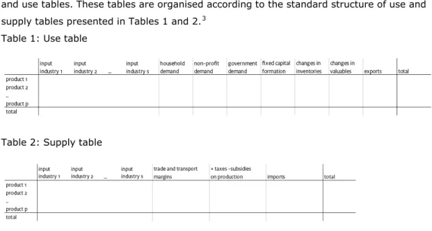
In the second step, the obtained national supply and use tables were regionalised. The main aim of this second step is to obtain, for every region, total exports and total imports, per product for the year 2010. This will be achieved by constructing consistent regional supply and use tables. These tables are organised according to the standard structure of use and supply tables presented in Tables 1 and 2.3
Table 1: Use table
Table 2: Supply table
These regionalised supply and use tables are conform the national supply and use tables used in WIOD (only the number of sectors is reduced to 14 because of data availability, see Table 3). This means that total use in the region would match total supply, which implies that the totals of the rows in the use table equals the totals of the rows in the supply table.
This equality is the regional version of the more familiar macroeconomic condition that production is equal to consumption plus exports minus imports. The totals of the columns in the regional supply and use tables are also equal because total output of every regional industry equals this industry’s total input and value-added. The regional supply and use tables give boundaries to the total regional exports and imports and are therefore crucial to infer regional export and import patterns.
We employed the approach known as the Commodity Balance (CB) method, first suggested by Isard (1953). National supply and use tables were crossed with regional data on value-added, regional investment, government demand and consumer demand (both with regional income as a proxy) from Eurostat (2014). Consistency of regional value-added, investment, government demand and consumer demand with the national account data in WIOD was obtained by multiplying the national value according to WIOD with the share of regions in the national totals. These data provided the necessary information on regional totals, without a distinction between different products. To disaggregate these totals into different products (the rows of the supply and use tables), the national supply and use tables were used. The structure of the national supply and use tables is assumed to give a good approximation for the regional tables. More formally, consumers are assumed to have homogenous preferences throughout the country concerned, homogenous government spending is assumed over the regions, and industries are assumed to use the same production technology, irrespective of their location within the country concerned.
Under these assumptions, regional household demand (HHD) per product (CPA, marked with index g), for example, is obtained according to Equation (2).
1 r r N g R N g r r
HHD
HHD
HHD
HHD
Î ==
å
,
(2)
where N stands for the country and R is the total number of regions within that country. In a comparable way regional production was determined. Since no information is available on regional total exports and imports from Eurostat, we used the regional value-added as a proxy for the regional trade shares in 2010. Exports and imports, therefore, were distributed across regions according to production and consumption shares as explained by
Equation (3). For instance, exports would be:
1 r g r N g R N g r g r VA X X VA Î = =
å
,
(3)
where X is exports and VA is value-added per region. It should be emphasised that this is only a first estimate of the international trade of regions, based on fixed shares. The ‘true’ amount of regional trade is determined in the updating method (step 3).
3.2.1 Production and consumption
In order to regionalise the national supply and use tables, we first distributed production and final demand over the regions. The regional demand in the use tables was divided into intermediate demand (input by industry), household demand, government demand, demand from non-profit organisations, gross fixed capital formation, changes in inventories, and changes in valuables.
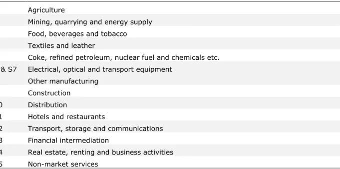
With respect to the supply tables, regional output had to be broken down by industries, trade and transport margins and net taxes. First, the data on production were determined per industry as well as the intermediate demand., Although no information is available on output at the European NUTS2 level, we did obtain data on value-added (VA) for 14 economic sectors from Eurostat. Table 3 presents the classification for these 14 economic sectors.
Table 3: Industry classification in 14 sectors S1 Agriculture
S2 Mining, quarrying and energy supply S3 Food, beverages and tobacco S4 Textiles and leather
S5 Coke, refined petroleum, nuclear fuel and chemicals etc. S6 & S7 Electrical, optical and transport equipment
S8 Other manufacturing S9 Construction
S10 Distribution
S11 Hotels and restaurants
S12 Transport, storage and communications S13 Financial intermediation
S14 Real estate, renting and business activities S15 Non-market services
Maintaining the index g for products and introducing the index s for sectors, regional output and input were constructed using information on value-added in the following way:
1 r r s N gs R N gs r s r
VA
input
input
VA
Î ==
å
(4)
1 r r s N gs R N gs r s rVA
output
output
VA
Î ==
å
(5)
This approach is based on two main assumptions. First, the production technology through which a sector transforms inputs into outputs is assumed to be homogeneous throughout the country considered. The regional shares of value-added in the national total of value added
represents a good proxy for the magnitude of the regional industries production shares in national output. In this way consistency per product is maintained, with the sum across regions of output (or input) per product and per industry equalling its national output (or input).
Second, the preferences of final consumers in each region are assumed to reflect preferences nation-wide. The regionalisation was done using Equation (2). Regional household demand was combined with the very small demand from non-profit organisations, since there was no regional information available on non-profit organisations. Regional income statistics were used as a proxy for the household demand. We also used household income as a proxy to regionalise total government demand per region. It is reasonable to assume that the expenditure of the government sector follows the economic size of the region. However, it should be emphasised that the regionalisation of government expenditure over the regions is only done to obtain a first starting point. The size of government expenditure in the region is endogenously determined as part of the optimisation. The demand pattern per product is assumed not to differ between regions, and is thus:
1 r r N g R N g r r Inc GOVD GOVD Inc Î = =
å
(6)
Where Inc represents the household income in the region.
Gross capital formation is divided into three items: gross fixed capital formation, changes in inventories and changes in valuables. With respect to the gross capital formation we used region information on investment to regionalise the national total capital formation. Investments were considered per region, therefore:
1 r r N g R N g r r
INV
INV
INV
INV
Î ==
å
(7)
Changes in inventories and valuables were made using regional value-added as a proxy. Just as in the case of the government demand and international trade this is only used as a first estimate and the final amount of regional expenditures on inventories and valuables is endogenously determined in the updating methodology. Hence, changes in inventories and valuables (CIV) were defined as:
1 r r N g R N g r r
VA
CIV
CIV
VA
Î ==
å
(8)
In a similar fashion, this last consideration could also be applied to the two remaining columns in the supply table: trade and transport margins (TTM) and taxes and subsidies (TAX). Since their regional variation is also assumed to be proportional to production, we defined them as:
1 r r N g R N g r r
VA
TTM
TTM
VA
Î ==
å
(9)
and 1 r r N g R N g r rVA
TAX
TAX
VA
Î ==
å
(10)
All data in the regionalised supply and use tables now are defined, except domestic trade, i.e., trade between regions of the same country. We used our PBL data set here as a first estimate. That is, we allocated, for example, the use of a product by an industry to regions in a country according to the intraregional trade of this product that is available in the original PBL trade database. Again, this is only a first proxy for the trade, since this is endogenously determined in the estimation procedure described in the next section.
3.3 Extrapolation of the 2000 regional trade matrix to
2010
Building on the unique database on bilateral trade between 256 European NUTS2 regions in 59 product categories for the year 2000 (Thissen et al., 2013b), as explained in the previous section, regional and national information for the year 2010 from Eurostat was used to extrapolate the data from 2000 to 2010. The resulting bi-regional data set describes the most likely trade flows between European regions, given all the available information, and is consistent with national accounts data as presented in the WIOD database.
The update of the data up until 2010 was based on constrained non-linear optimisation. The objective function in the non-linear optimisation minimised the quadratic distances between the coefficients of the regional SAM matrix in relation to the coefficients of the national SAM matrix given regional data on value-added, fixed capital formation and household demand. The optimisation was constrained in such a way that all cells of the regional supply and use tables add up over the regions to the national cells presented in the WIOD supply and use tables. Moreover, by imposing the constraint that all exports of a region should be equal or smaller than production it is not possible to have regional re-exports.
The size of the constrained non-linear minimisation problem is such that the procedure was divided into two steps. In a first step, domestic trade and international trade from regions to countries was determined. In this step also the regional supply and use tables were
determined. The second step involved subdividing the international trade from European regions to countries into trade between regions. Throughout this process, all normal
consistency rules were applied, so that the amount of products exported from one region to another (destination) region or country would equal the amount imported into that
destination region or country from that particular region of origin. Re-exports were not allowed on the regional level.
The methodology for constructing the updated data set is outlined in more detail in the next sections.
3.3.1 Regionalising IO or supply and use Tables
Central in our analysis is regionalisation of the WIOD supply and use framework. We use a supply and use framework rather than an Input-Output framework, because the focus is on the regionalisation both trade and regional technological coefficients (the use and supply of products by different economic actors). An input-output framework is built around the assumption that every sector produces only one good. There are two basic approaches to construct a supply and use framework and therefore there are two types of input-output matrices: product-by-product matrices and sector-by-sector matrices. Product-by-product input-output matrices have been constructed around the product classification and sectors are therefore adjusted or mixed in such a way that only one sector makes only one product. Sector-by-sector input-output matrices have been constructed around the sector
classification and products are therefore adjusted or mixed in such a way that only one sector makes only one product. This implies that, depending on the type of IO table, either the sectors are not comparable over the nations and not comparable with regional sector statistics, or products are not comparable over nations and not comparable with trade statistics. Hence, a regionalisation of IO tables can either only be based on regional sector statistics or only on regional trade statistics. We intended to use both a regional trade database and production and consumption data of different actors in different regions. As a consequence is the regionalisation of a complete supply and use framework the only option available to us.
3.3.2 Interregional social accounting matrix (SAM)
For the sake of convenience, the supply and use data were first entered into a social accounting matrix (SAM) framework (SNA, 1993; 2008). Using such a complete national accounts framework in matrix format, has the advantage that all consistency checks can be performed immediately. Thus, the imported amount of product into region B from region A is, per definition, exactly the same as the exported amount of this product from region A to region B, as this amount is recorded in only one position in the matrix. In general, valuations in a SAM are in nominal terms. Its rows and columns list institutional agents or actors. The matrix shows the flow of goods between actors, from row to column, balanced by an opposite flow of money from column to row. The SAM framework also illustrates the
methodology used. We used more recent information from national and regional accounts to impose requirements that had to be met while minimising any structural distance to the elements of the matrix on which no new information was available. Here we see that changes in regional demand or production have a direct impact on regional trade, because
what is exported must be produced and what is imported should represent demand. This minimisation of the structural distance is applied by keeping the changes in the relative numbers of the matrix to a minimum. The consistency of the system of national and regional accounts in a SAM framework, therefore, provides a large amount of information on regional trade developments.
Figure 2: A stylised interregional Social Accounting Matrix
A stylised version of the SAM is presented in Figure 2, which distinguishes two regions. The SAM consists of a framework in which the use table is combined with the transposed supply table. The two regions distinguished in the SAM have two sectors, 1 and 2, producing two types of products. A product in the SAM, thus, has three characteristics: type of good, the region and the sector of production. The use of this product by different sectors in different regions is presented in the first four columns of the SAM. The production of these products is presented on the top 4 rows of the SAM. Total production in these sectors is provided in the last column on the right. In the bottom two rows we find the total value-added which is an aggregation of both labour and capital income.
Table 4: Non-Industrial actors and other accounts distinguished in the SAM
S16 Final consumption expenditure by households and non-profit organisations S17 Final consumption expenditure by government
S18 Net capital formation S19 Inventory adjustment S20 Trade and transport margins S21 Taxes less subsidies on products S22 Exports (outside Europe)
S23 Imports (outside Europe)
International trade takes place at the product level and is divided over different types of use. The use of the final demand categories is presented in the last two columns of the SAM. The use by the different producing sectors is presented in the first two columns. Thus, Region 1 exports a total of 3 units of product 2 to Region 2, 2 of which are used by Sector 2 and 1 unit is used by the final demand categories. The final demand for goods per region does not equal the total value-added earned in that same region. Only when interregional savings would be
Region 1: Use Region 2: Use Region 1: Supply Region 2: Supply Region 1: Use Region 2: Use sector 1 sector 2 sector 1 sector 2 product 1 product 2 product 1 product 2 hhd - Investment hhd - investment
Region1 sector 1 3 7 10 sector 2 2 6 8 Region 2 sector 1 5 2 7 sector 2 3 6 9 Region 1 product 1 1 1 1 1 1 5 product 2 2 3 2 5 1 13 Region 2 product 1 1 2 1 4 8 product 2 1 1 6 8
Region 1 value added 6 3 transfer transfer
Region 2 value added 4 6 transfer transfer 19
10 8 7 9 5 13 8 8 19 x
SAM
total
specified in the transfer part of the SAM these would be equal. In our SAMs we do not specify the transfer part, because we have no information on these flows and we do not need them in our updating procedure. In our stylised presentation of the SAM, therefore, all added rows and all final demand columns were added to obtain equality between total value-added and total final demand. All other rows add up to the same respective columns
representing the bookkeeping rules that for every actor total expenditure should equal total income.
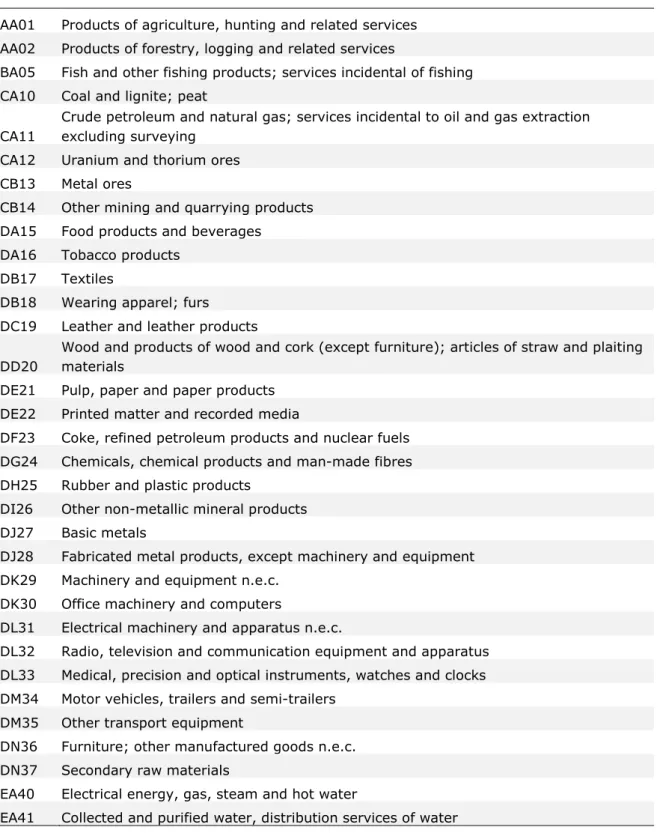
Table 5: The 2-digit Classification of Products by Activity (CPA, 1996)
AA01 Products of agriculture, hunting and related services AA02 Products of forestry, logging and related services
BA05 Fish and other fishing products; services incidental of fishing CA10 Coal and lignite; peat
CA11
Crude petroleum and natural gas; services incidental to oil and gas extraction excluding surveying
CA12 Uranium and thorium ores CB13 Metal ores
CB14 Other mining and quarrying products DA15 Food products and beverages
DA16 Tobacco products DB17 Textiles
DB18 Wearing apparel; furs DC19 Leather and leather products
DD20
Wood and products of wood and cork (except furniture); articles of straw and plaiting materials
DE21 Pulp, paper and paper products DE22 Printed matter and recorded media
DF23 Coke, refined petroleum products and nuclear fuels DG24 Chemicals, chemical products and man-made fibres DH25 Rubber and plastic products
DI26 Other non-metallic mineral products DJ27 Basic metals
DJ28 Fabricated metal products, except machinery and equipment DK29 Machinery and equipment n.e.c.
DK30 Office machinery and computers
DL31 Electrical machinery and apparatus n.e.c.
DL32 Radio, television and communication equipment and apparatus DL33 Medical, precision and optical instruments, watches and clocks DM34 Motor vehicles, trailers and semi-trailers
DM35 Other transport equipment
DN36 Furniture; other manufactured goods n.e.c. DN37 Secondary raw materials
EA40 Electrical energy, gas, steam and hot water
FA45 Construction work
FA50
Trade, maintenance and repair services of motor vehicles and motorcycles; retail sale of automotive fuel
GA51
Wholesale trade and commission trade services, except of motor vehicles and motorcycles
GA52
Retail trade services, except of motor vehicles and motorcycles; repair services of personal and household goods
HA55 Hotel and restaurant services
IA60 Land transport; transport via pipeline services IA61 Water transport services
IA62 Air transport services
IA63 Supporting and auxiliary transport services; travel agency services IA64 Post and telecommunication services
JA65 Financial intermediation services, except insurance and pension funding services JA66 Insurance and pension funding services, except compulsory social security services JA67 Services auxiliary to financial intermediation
KA70 Real estate services
KA71
Renting services of machinery and equipment without operator and of personal and household goods
KA72 Computer and related services KA73 Research and development services KA74 Other business services
LA75 Public administration and defence services; compulsory social security services MA80 Education services
NA85 Health and social work services
OA90 Sewage and refuse disposal services, sanitation and similar services OA91 Membership organisation services n.e.c.
OA92 Recreational, cultural and sporting services OA93 Other services
PA95 Private households with employed persons
Our regional SAMs distinguish the 14 industry categories presented in Table 3, and the non-Industrial actors and other accounts presented in Table 4. Products are classified according to the 2-digit Classification of Products by Activity (CPA, 1996) presented in Table 5. There is a total of 62 goods and services in CPA 2002. Yet, products with numbers 96, 97 and 99 (goods produced by households for own use, services produced by households for own use and services provided by extra-territorial organisations and bodies) are not included in the supply and use system of accounts, reducing the total number of products analysed in this study to 59.
3.3.3 First step: domestic trade and international trade between regions
and countries
In this first step, we used constrained non-linear optimisation to determine the trade of regions with regions within the same country, and the international trade between these regions and other countries.
The objective function in the first step of the extrapolation
Equation (11) shows the linear quadratic objective function to be minimised in our non-linear optimisation problem The function describes how new information is used to find updated matrices, given the growth in production and demand indicated in the national and regional accounts. In general, the change in the structure of the demand, supply and regional trade pattern was minimised, given new information on for instance regional value-added and international trade. The complete minimisation problem can be described as follows.
(
) (
2) (
2ˆ
)
2ˆ
ˆ
constraints
c c r r i i i i i i i cMin Z
a
a
a
a
t
t
Îé
ù
=
ê
-
+
-
+
-
ú
ê
ú
ë
û
+
å
(11)
Where the index
i
stands for the region, c ia represents the elements of the regional SAM matrix divided by its column total, r
i
a represents the elements of the regional SAM matrix divided by its row total, and ti stands for the international trade margins divided by the total exports per product. For matters of convenience we left out the summation over the
elements of the SAM matrix. The SAM matrix is aggregated for all the imports from regions and countries except the regions from the own country. Thus in this first step of the procedure only the domestic trade and non-trade coefficients of the regional SAM matrices are determined. The international trade is determined in the second step of the procedure. As a consequence the first step in the procedure can be done for all countries separately.
The constraints on the objective function
The objective function was constrained to generate outcomes conform the regional and national accounts in WIOD. Moreover, economic theory was used to derive information which was implemented in the procedure by adding additional constraints. The most common additional information derived from theory was the non-negativity condition of trade flows. The limitation to only have positive trade values guaranteed that all goods had a positive price and were therefore valued with a positive number in the SAM. Below, all constraints used are discussed along with the information they contain.
1. All elements summed over all regions in a country add up to the same elements in the national WIOD-based SAM. This constraint guarantees that the regional SAMs are completely compatible with the WIOD database.
2. All products sold by an economic agent are received and paid for by another economic agent. This bookkeeping rule was adhered to by imposing the equality of
all row and column totals of the SAM for all activities (classified according to industry) and products.
3. Information was available on regional value-added for the distinguished industries. Value-added of the sectors in the regions was therefore fixed.
4. Information was available on regional total household demand and regional total gross fixed capital formation. These items have therefore been fixed also in the procedure.
5. Finally, a 'no re-export' constraint was applied to ensure that production would always exceed exports, for every region and product. Please note that this constraint should be imposed on the product level and not on the industry level.
Solving the minimisation problem under these constraints resulted in the update of the regional SAM, including domestic trade from the year 2000 to the year 2010.
3.3.4 Second step: international trade between regions
The international trade between regions of European countries was determined in the first step of the procedure, described above. In the second step, these international trade flows were subdivided into regions of destination and regions of origin, resulting in a full regional origin–destination matrix. No additional information was available on these trade patterns, except on international trade between countries. We used constrained non-linear quadratic optimisation to combine this information with existing trade patterns to determine the final panel data on trade between NUTS2 regions for the 2000–2010 period.
The most important part of the supply and use framework are the technical coefficients. These coefficients are crucial in, for instance, Input-output analysis. Hence, it makes sense to minimise the quadratic error of these coefficients. However, with respect to trade this is different. Absolute values are just as important as relative values. We therefore applied a mixed objective function where a quadratic absolute ae and a quadratic relative error re
were both minimised simultaneously. Two priors were taken into account: one being the estimated trade from an export perspective, and the other from an import perspective.
This gives the following objective function:
(
)
(
)
(
)
(
)
' 2 2 , , , , , , , , , , , , 2 2 , , , , , , , , , , , , , , , , , , , ,. .
1
ˆ
1
ˆ
1
ˆ
1
ˆ
ˆ
ˆ
s s s ex ex im im s ex s i j s i j im s i j s i j i j i j i j i j ex ex im im s ex s i j s i j im s i j s i j i j i i j j ex c d s s i j i c j d ex s d c s i j i c j dMin Z
re
ae
s t
re
ae
Ex
Im
t
t
t
t
t
t
t
t
t
t
t
t
t
t
Î Î Î Î=
+
=
-
+
-=
-
+
-=
=
å
å
å
å
å
å
å
(12)
in which Exc d, denotes exports of country
c
destined for countryd
(directly taken from the WIOD tables) and Imj c, denotes imports in countryd
from countryc
(directly taken from the WIOD tables). The regional trade estimation is performed on the importing sector level (s
) and thereby completely consistent with the WIOD tables. The priors of exports (imports) were determined by the regional trade pattern of exports (imports) from the year 2000. Please note that we defined the quadratic relative error slightly different than inpercentages.4 The reason is related to the weight of both errors in the objective function. In
the above specification, both weights are exactly the same because the sum of trade between all regions ex,
i j
t
is equal to the sum over all regions of the average value of the tradeex i
t .
3.4 Additional regions
Lastly, 30 NUTS2 regions that were not in the PBL data set were added to the 256 NUTS2 regions to obtain the complete trade data set for the EU27. The missing regions were all regions in Romania, Bulgaria and Slovenia. Slovenia was recently split into two regions and therefore still presented as one region in the PBL database. Additionally, the Islands of Portugal were included in the database constructed for IPTS and Denmark was changed in a different regional classification.
The same methodology has been used to obtain the trade for these regions missing from the PBL data set. In all cases the trade was already available at the country level. Thus, all regions available in the PBL database already traded with the countries. The only thing we had to do is subdivide this trade over the different regions in these countries. We used the share from the external IPTS gravity estimation database to obtain the trade data for the regions in these countries. Thus, for instance, trade from Andalusia to Romania was subdivided over the Romanian regions according to the proportions taken from the gravity-based IPTS database. Exactly the same approach was followed to subdivide the imports. Finally, the internal trade between the missing regions from the same country was subdivided according to the trade patterns in the IPTS gravity-based trade database. For example, the proportions of domestic trade were obtained by dividing the Romanian
domestic trade from the gravity-based IPTS trade database by the total Romanian domestic trade. The domestic trade in the new database was subsequently obtained by multiplying these proportions with the domestic trade as given in the WIOD database.
4A relative error based on percentage would have been as follows:
2(
)
2 2(
)
2 , , , , , , , , , , , , , , ,1
1
ˆ
ex exˆ
im im s ex s i j s i j im s i j s i j i j s i j s i j s i jre
t
t
t
t
t
t
æ
ö
÷
æ
ö
÷
ç
÷
ç
÷
ç
ç
=
ç
ç
÷
÷
-
+
ç
ç
÷
÷
-÷
÷
÷
÷
ç
ç
è
ø
è
ø
å
å
.4 Conclusions
This paper describes the construction of a database on regional trade between all NUTS2 regions in the EU27. The methodology used was based on an extrapolation of the PBL trade database for 2000 to 2010, using new regional information. The resulting regional data set describes the most likely trade flows between European regions, given all the available information, and is consistent with national accounts. The ensuing data are also fully consistent with international trade between the Member States and with the rest of the world, for the 6 product categories used in the Rhomolo model.
5 References
Dietzenbacher E, Los B, Steher R, Timmer MP and De Vries GJ. (2013). The Construction of World Input-Output Tables in the WIOD Project. Economic Systems Research, 25: 71–98. Feenstra RC, Lipsey RE, Deng H, Ma AC and Mo H. (2005). World Trade Flows: 1962–2000.
National Bureau of Economic Research.
Isard W. (1953). Regional commodity balances and interregional commodity flows. American Economic Review 43: 167–80.
Lankhuizen M and Thissen M. (2014). Identifying true trade patterns: correcting bilateral trade flows for re-exports, 22nd IIOA Conference, Lisbon.
Simini F, González MC, Maritan A and Barabási A. (2012). A universal model for mobility and migration patterns, Nature, 484, pp. 96–100, doi:10.1038/nature10856.
Stone R. (1963). Input–output relationships 1954–1966, The department of applied economics University of Cambridge, Chapman and Hall, Cambridge.
System of National Accounts (1993 and 2008). System of National Accounts (SNA). United Nation website: http://unstats.un.org/unsd/nationalaccount/sna.asp
Timmer MP. (ed) (2012). ‘The World Input–Output Database (WIOD): Contents, Sources and Methods’, WIOD Working Paper Number 10, downloadable at
http://www.wiod.org/publications/papers/wiod10.pdf
Thissen M and Löfgren H. (1998). A new approach to SAM updating with an application to Egypt, Environment and Planning A 30: 1991–2003.
Thissen M, Van Oort F, Diodato D and Ruijs A. (2013a). European regional competitiveness and Smart Specialization; Regional place-based development perspectives in international economic networks, Cheltenham: Edward Elgar.
Thissen M, Diodato D and Van Oort F. (2013b). Integrated regional Europe: European regional trade flows in 2000. PBL Netherlands Environmental Assessment Agency, The Hague.
Thissen M, Diodato D and Van Oort F. (2013c). European regional trade flows: An update for 2000–2010. PBL Netherlands Environmental Assessment Agency, The Hague.
Appendix A: Estimating
trade flows not
including re-exports
A.1 Determining the re-exports matrices
We derived the following variables from the WIOD supply and use tables:
1. REi p, Re-exports RE per country i and product p excluding trade margins. 2. Ti j p, , Imports of product p by country j coming from country i excluding
trade margins.
3. ITMi j p, , The international trade margin in imports of product p by country j coming from country i.
4. IMj p, Imports by country j excluding trade margins. 5. Exi p, Exports from country i excluding trade margins.
Under the assumption of the same import patterns of imports and re-exports we have the following probabilities of the origin of imports PIi j p, , and destination of exports PEi j p, , :
6. , , , , ', , ' i j p i j p i j p i
T
PI
T
=
å
probabilities of the origin of imports7. , , , , , ', ' i j p i j p i j p j
T
PE
T
=
å
probabilities of the destination of exportsWe want to determine the re-exports table REODi q j p, , , describing the re-export of product p coming from country i, re-exported by country q, and with final destination country j. To determine this re-exports table REODi q j p, , , we minimise Z
(
)
2(
)
2(
)
2 , , , , , , , , , , , , , , ˆi q p ˆ'q j p ˆi q j p i q p q j p i q j p Z =å
e +å
e +å
e (13)under the following constraints. First of all, the errors eˆi q p, , , eˆ'q j p, , and eˆi q j p, , , are determined by the following equations:5
, , , , , ˆ, , i q p i q p q p i q p REO =PI RE +e (14) , , , , , ˆ', , q j p q j p q p q j p RED =PE RE +e (15) , , , , , , , , , , ,
ˆ
i q p i q j p q j p i q j p q pREO
REOD
RED
e
RE
=
+
(16)Equations (14) and (15) describe the origin REOi q p, , and the destination REDq j p, , of the re-exports. Equation (16) specifies that re-exports are determined endogenously. Moreover, the system will be solved under the conditions that re-exports attributed to some origin i can never exceed total exports from that country, and that re-exports to a destination j cannot exceed the imports of that country. That is,
, , , i q p i p q REO £Ex
å
(17) , , , q j p j p q RED £IMå
(18)The quadratic minimisation (13) under the constraints (14), (15), (16), (17) and (18) will give us the re-export matrices REODi q j p, , , .
We can subsequently use these matrices REODi q j p, , , to determine trade matrices TREi j p, ,
that are cleaned from re-exports. The starting point are the trade matrices given in the WIOD where re-exports have already been taken out of imports. The only thing we have to do is adjust the WIOD trade tables by changing the origin of the re-exported imports. Thus, first we subtract the re-exported imports from the original trade tables at their final
destination and we subsequently add all the ‘true’ origins of these re-exports. This is explained by the following equation:
, , , , , , , , ,
i j p i j p i j p i q j p q
TRE =T -RED +
å
REOD (19)A.2. Closing the system: exports equal imports
We know that total imports coming from a certain origin cannot exceed the exports of that origin. Therefore, the following condition should be satisfied (please note that in this
5 We minimise both absolute and relative errors. The latter serves to ensure small trade flows are not increased
formulation any difference between exports and imports from other countries is going to the rest of the world):
, , ,
i p i j p j
Ex ³
å
TRE (20)This gives the following condition that has to be added to the estimation of the re-exports that can be obtained by substituting (16) and (19) into (20).
, , , , , , , , , , i q p i p i j p i j p q j p j q q p
REO
Ex
T
RED
RED
RE
æ
ö÷
ç
÷
ç
³
ç
ç
-
+
÷
÷
÷
çè
ø
å
å
(21)Please note that this constraint is non-linear and including this constraint will change the problem from a quadratic (or conic) minimisation problem into a non-linear minimisation problem.
The degree that exports of a country are larger than the sum of the imports coming from that country to all the other distinguished countries is due to missing exports to the rest of the world. These can therefore be booked as such.
A.3. International trade margins
WIOD lists international trade margins ITMi j p, , separately. These trade margins also have to be corrected for re-exports. The international trade margins cleaned from re-exports are estimated simultaneously with the estimation of re-exports by using the fact that total imports cif of product p by a country (in the supply table) are equal to imports in basic prices plus re-exports plus international trade margins. Hence,
, , , , , , , , , , , ,
1
i j p j p i j p i j p i q j p j i j p qITM
IMcif
T
RED
REOD
T
ææ
ö
÷
æ
ö
÷
ö
÷
çç
÷
ç
÷
÷
çç
ç
=
å
çç
èè
çç
çç
+
÷
ø
÷
÷
*
ç
ç
è
-
+
å
÷
÷
÷
ø
÷
ø
÷
÷
(22)It is assumed that the share of trade margin in the total trade, , , , ,
i j p i j p
ITM
T
, is constant.A.4. The complete minimisation problem
The minimisation problem needed to determine the re-export tables consists therefore of the minimisation of Z in Equation (13) under the constraints (14), (15), (16), (17), (18), (21) and (22). The minimisation resulted in the complete re-export matrices and the new trade tables between countries for 59 product categories.
A.5. Disaggregating trade over demand categories
Unfortunately there is no information that distinguishes the different demand categories. We therefore can only apply the above mentioned methodology for total trade of different product categories. Thus in a last step we have to divide this trade and the associated ITMs over the different demand categories. This is a typical RAS (Stone, 1963) problem where given prior knowledge about the content of a matrix (the old WIOD database) a new matrix has to be constructed given new information on the totals. This methodology is also known as a bi-proportional updating method and can be shown to be exactly the same as an Entropy minimisation (Thissen and Lofgren, 1998). We used the methodology described by Thissen and Lofgren (1998) to update the matrices and obtained new estimates for both the trade and the international trade margins divided over the different demand categories.
Appendix B: The
region and product
classification of the
trade data set
The constructed trade data set follows the standard CPA product classification in main categories and the NUTS2 regional classification for the EU27. Both classifications are presented in Tables B.1 and B.2.
Table B.1: The Rhomolo Classification and the Classification of Products by Activity (CPA, 2002)
Rhomolo
Classification CPA Name
AB A PRODUCTS OF AGRICULTURE, HUNTING AND FORESTRY
B FISH AND OTHER FISHING PRODUCTS; SERVICES INCIDENTAL TO FISHING CDE C PRODUCTS FROM MINING AND QUARRYING
D MANUFACTURED PRODUCTS
E ELECTRICAL ENERGY, GAS, STEAM AND WATER
F F CONSTRUCTION WORK
GHI G WHOLESALE AND RETAIL TRADE SERVICES;
REPAIR SERVICES OF MOTOR VEHICLES, MOTORCYCLES AND PERSONAL AND HOUSEHOLD GOODS
H HOTEL AND RESTAURANT SERVICES
I TRANSPORT, STORAGE AND COMMUNICATION SERVICES JK J FINANCIAL INTERMEDIATION SERVICES
K REAL ESTATE, RENTING AND BUSINESS SERVICES LMNOPQ L PUBLIC ADMINISTRATION AND DEFENCE SERVICES;
COMPULSORY SOCIAL SECURITY SERVICES M EDUCATION SERVICES
N HEALTH AND SOCIAL WORK SERVICES
O OTHER COMMUNITY, SOCIAL AND PERSONAL SERVICES P SERVICES OF HOUSEHOLDS
Q SERVICES PROVIDED BY EXTRA-TERRITORIAL ORGANIZATIONS AND BODIES
Table B.2 The Rhomolo regional classification derived from the Nuts2 classification
Code Name Code Name Code Name
AT11 Burgenland FI1A Pohjois-Suomi PL51 Dolnoslaskie
AT12 Niederosterreich FI20 Aland PL52 Opolskie
AT13 Wien FR10 Ile de France PL61 Kujawsko-Pomorskie
AT21 Karnten FR21 Champagne-Ardenne PL62 Warminsko-Mazurskie
AT22 Steiermark FR22 Picardie PL63 Pomorskie
AT31 Oberosterreich FR23 Haute-Normandie PT11 Norte
AT32 Salzburg FR24 Centre PT15 Algarve
AT33 Tirol FR25 Basse-Normandie PT16 Centro (PT)
AT34 Vorarlberg FR26 Bourgogne PT17 Lisboa
BE10 Region de Bruxelles FR30 Nord - Pas-de-Calais PT18 Alentejo
BE21 Prov. Antwerpen FR41 Lorraine PT20 Região Autónoma dos Açores
BE22 Prov. Limburg (B) FR42 Alsace PT30 Região Autónoma da Madeira
BE23 Prov. Oost-Vlaanderen FR43 Franche-Comte SE11 Stockholm
BE24 Prov. Vlaams Brabant FR51 Pays de la Loire SE12 ostra Mellansverige
BE25 Prov. West-Vlaanderen FR52 Bretagne SE21 Sydsverige
BE31 Prov. Brabant Wallon FR53 Poitou-Charentes SE22 Norra Mellansverige
BE32 Prov. Hainaut FR61 Aquitaine SE23 Mellersta Norrland
BE33 Prov. Liege FR62 Midi-Pyrenees SE31 ovre Norrland
BE34 Prov. Luxembourg (B) FR63 Limousin SE32 Småland med oarna
BE35 Prov. Namur FR71 Rhone-Alpes SE33 Västsverige
CZ01 Praha FR72 Auvergne SK01 Bratislavský kraj
CZ02 Stredni Cechy FR81 Languedoc-Roussillon SK02 Zapadne Slovensko
CZ03 Jihozapad FR82 Provence-Alpes-Cote d Azur SK03 Stredne Slovensko
CZ04 Severozapad FR83 Corse SK04 Východne Slovensko
CZ05 Severovychod GR11 Anatoliki Makedonia Thraki UKC1 Tees Valley and Durham
CZ06 Jihovychod GR12 Kentriki Makedonia UKC2 Northumberland Tyne and
Wear
CZ07 Stredni Morava GR13 Dytiki Makedonia UKD1 Cumbria
CZ08 Moravskoslezko GR14 Thessalia UKD2 Cheshire
DE11 Stuttgart GR21 Ipeiros UKD3 Greater Manchester
DE12 Karlsruhe GR22 Ionia Nisia UKD4 Lancashire
DE13 Freiburg GR23 Dytiki Ellada UKD5 Merseyside
DE14 Tubingen GR24 Sterea Ellada UKE1 East Riding, North Lincolnshire
DE21 Oberbayern GR25 Peloponnisos UKE2 North Yorkshire
DE22 Niederbayern GR30 Attiki UKE3 South Yorkshire
DE23 Oberpfalz GR41 Voreio Aigaio UKE4 West Yorkshire
DE24 Oberfranken GR42 Notio Aigaio UKF1 Derbyshire and
Nottinghamshire
DE25 Mittelfranken GR43 Kriti UKF2 Leicestershire Rutland
DE26 Unterfranken HU10 Kozep-Magyarorszag UKF3 Lincolnshire
DE27 Schwaben HU21 Kozep-Dunantul UKG1 Herefordshire Worcestershire
DE41 Brandenburg - Nordost HU23 Del-Dunantul UKG3 West Midlands
DE42 Brandenburg - Südwest HU31 eszak-Magyarorszag UKH1 East Anglia
DE50 Bremen HU32 eszak-Alfold UKH2 Bedfordshire Hertfordshire
DE60 Hamburg HU33 Del-Alfold UKH3 Essex
DE71 Darmstadt IE01 Border Midlands UKI1 Inner London
DE72 Giessen IE02 Southern and Eastern UKI2 Outer London
DE73 Kassel ITC1 Piemonte UKJ1 Berkshire Bucks Oxfordshire
DE80 Mecklenburg-Vorpommern ITC2 Valle dAosta Vallee dAoste UKJ2 Surrey East and West Sussex
DE91 Braunschweig ITC3 Liguria UKJ3 Hampshire and Isle of Wight
DE92 Hannover ITC4 Lombardia UKJ4 Kent
DE93 Luneburg ITD1 Bolzano-Bozen UKK1 Gloucestershire Wiltshire
DE94 Weser-Ems ITD2 Provincia Autonoma Trento UKK2 Dorset and Somerset
DEA1 Dusseldorf ITD3 Veneto UKK3 Cornwall and Isles of Scilly
DEA2 Koln ITD4 Friuli-Venezia Giulia UKK4 Devon
DEA3 Munster ITD5 Emilia-Romagna UKL1 West Wales and The Valleys
DEA4 Detmold ITE1 Toscana UKL2 East Wales
DEA5 Arnsberg ITE2 Umbria UKM2 North Eastern Scotland
DEB1 Koblenz ITE3 Marche UKM3 Eastern Scotland
DEB2 Trier ITE4 Lazio UKM5 South Western Scotland
DEB3 Rheinhessen-Pfalz ITF1 Abruzzo UKM6 Highlands and Islands
DEE0 Saarland ITF2 Molise UKN0 Northern Ireland
DED1 Chemnitz ITF3 Campania BG31 Severozapaden
DED2 Dresden ITF4 Puglia BG32 Severen tsentralen
DED3 Leipzig ITF5 Basilicata BG33 Severoiztochen
DEF0 Schleswig-Holstein ITF6 Calabria BG34 Yugoiztochen
DEG0 Thüringen ITG1 Sicilia BG41 Yugozapaden
DK01 Hovedstadsreg ITG2 Sardegna BG42 Yuzhen tsentralen
DK02 Ost for Storebælt LT00 Lietuva CY00 Kypros/Kıbrıs
DK03 Syddanmark LU00 Luxembourg (Grand-D) SI01 Vzhodna Slovenija
DK04 Midtjylland LV00 Latvija SI02 Zahodna Slovenija
DK05 Nordjylland MT00 Malta RO11 Nord-Vest
EE00 Eesti NL11 Groningen RO12 Centru
ES11 Galicia NL12 Friesland RO21 Nord-Est
ES12 Principado de Asturias NL13 Drenthe RO22 Sud-Est
ES13 Cantabria NL21 Overijssel RO31 Sud – Muntenia
ES21 Pais Vasco NL22 Gelderland RO32 Bucureşti – Ilfov
ES22 Foral de Navarra NL23 Flevoland RO41 Sud-Vest Oltenia
ES23 La Rioja NL31 Utrecht RO42 Vest
ES24 Aragon NL32 Noord-Holland JPN Japan
ES30 Comunidad de Madrid NL33 Zuid-Holland BRA Middle and South America
ES41 Castilla y Leon NL34 Zeeland AUS Austrialia and Oceania
ES42 Castilla-la Mancha NL41 Noord-Brabant MEX Northern America
ES43 Extremadura NL42 Limburg (NL) RUS Russia
ES51 Cataluna PL11 Lódzkie BGR Bulgaria
ES52 Comunidad Valenciana PL12 Mazowieckie ROU Roumania
ES61 Andalucia PL22 Slaskie IDN Indonesia
ES62 Region de Murcia PL31 Lubelskie CAN Canada
ES63 Ceuta (ES) PL32 Podkarpackie CHN China
ES64 Melilla (ES) PL33 Swietokrzyskie KOR Korea
ES70 Canarias (ES) PL34 Podlaskie TUR Turkey
FI13 Ita-Suomi PL41 Wielkopolskie USA United States
FI18 Etela-Suomi PL42 Zachodniopomorskie TWN Taiwan