Assessing the importance of individual modelling decisions for invasive range forecasting - A case study using the common waxbill

Biology Department

Research Group Terrestrial Ecology Unit

_____________________________________________________________________________________

ASSESSING THE IMPORTANCE OF INDIVIDUAL

MODELLING DECISIONS FOR INVASIVE

RANGE FORECASTING

A CASE STUDY USING THE COMMON WAXBILL

Marie Stessens

Supervisor(s): Dr. Diederik Strubbe Dr. Amy Davis

TABLE OF CONTENTS

1. Introduction ……….…..……..

1.1. Invasive Species ……….………. 1

1.2. Species Distribution Models ……….………..…….. 1

1.2.1. Definition ……….…….……. 1

1.2.2. Restricting model assumptions ……….…………. 2

1.2.3. Influential modelling choices ………...………… 2

1.2.3.1. Variable Selection ……….……….. 2

1.2.3.2. Background and Pseudo-absence selection ………….….……….. 3

1.2.3.3. Subspecific niche variation ……….…….……… 4

1.3. The Common waxbill ………..……… 4

1.3.1. Species information ………...……….. 4

1.3.2. A case study for invasiveness ……… 4

2. Objectives ……….. 6

3. Methodology ……….

7

3.1. Workflow overview ……….. 7

3.2. Baseline model construction ……….………. 8

3.2.1. Ensemble Forecasting ………. 8

3.2.2. Occurrence Data ………. 8

3.2.3. Explanatory variables ……….. 9

3.2.4. Spatially blocked cross-validation ……….. 10

3.2.5. Model evaluation ……….. 11

3.2.6. Environmental similarity ……….. 12

3.3. Variable selection strategies ……….. 12

3.3.1. Ecology based ……….. 12

3.3.2. Correlation based ……….. 12

3.3.3. ENFA – Ecological niche factor analysis ………..…….. 13

3.3.4. MESS – Multivariate environmental similarity surface ……… 13

3.4. Background Selection ……….. 13

3.4.1. Zoogeographical region ………. 13

3.4.2. Buffered presences ……….. 14

3.4.3. Predefined probability of absence ………. 14

3.4.4. Target group approach ……….. 14

3.5. Subspecific niche variation ……….. 15

3.5.1. Morphological differentiation ……….…. 15

3.5.1.1. Museum measurements ……….. 15

3.5.1.2. Morphometric analysis ………. 15

3.5.2. Subspecific Occurrences ……….. 16

3.5.3. Niche differentiation ……….. 16

4. Results ……….…… 18

4.1. Overall prediction success ……….…. 18

4.2. Effect of variable selection ……….… 19

4.3. Effect of background selection ………... 19

4.4. Accounting for subspecific niche variation ……….…… 20

4.4.1. Assessment of subspecific differentiation ……….…. 20

4.4.2. Effect of incorporating subspecies ………... 21

4.5. Environmental similarity ……….. 23

4.6. Variable Importance ………..….. 24

5.

Discussion

5.1. Overall species-level model accuracy ……….………. 25

5.1.1. Transferability to non-analogue climates……….…………. 26

5.1.2. Restricting SDM assumptions ………..… 26

5.2. Effect of variable selection ………. 28

5.2.1. Correlation ………...……. 28

5.2.2. MESS ……….………. 28

5.2.3. Ecology ………. 29

5.2.4. ENFA ……….…. 29

5.3. Effect of background selection ……….……… 29

5.4. Subspecific niche differentiation ………..….… 30

5.5. Variable Importance ……….………..…… 31

5.6. Context dependence of prediction success ……….… 32

6. Conclusion ……….………….. 33

7. Acknowledgments ……….. 34

8. Summary ……….….. 35

9. Samenvatting ……….. 38

1. INTRODUCTION

1.1. Invasive species

The distribution of species constantly changes as a result of natural processes such as changing climatic or resource conditions (Cracraft, 1994). Range boundaries of species are therefore inherently dynamic. Since recent times however, trade and transport accelerated these natural processes drastically. Humans exported an innumerable amount of species to areas that biogeographical boundaries naturally would forbid (Hulme, 2009). These deliberate or coincidental introductions are not always harmless. On the contrary, the introduction of invasive species globally ranks among top threats to biodiversity and severely endangers local ecosystems and their biotic interactions (Bellard et al., 2017; Butchart et al., 2010; McGeoch et al., 2010). Through competition, predation or disease spreading, they can directly impact native species. Invasive species also indirectly influence the welfare of other species by changing the abiotic environment and nutrient cycling processes (Cameron et al., 2016; Kenis et al., 2008). Besides damage to natural ecosystems, the economic ramifications of alien invasions are enormous (Vilà et Hulme, 2017). Multiple examples exist of invasive species causing economic harm by damaging infrastructure, decreasing agricultural yields or harming commercial forestry (Hanley & Roberts, 2019). The severe problems associated with these invaders are not transient. On the contrary, the number of alien species continues to rise (Lambertini et al., 2011; Seebens et al., 2017).

Among all invaders, birds are one of the most ubiquitous groups (Blackburn et al., 2009). Close to 420 bird species have established viable populations outside their home range as a result of human interference (Dyer et al., 2017). Although impacts of bird invasions were previously thought to be insignificant, more and more studies highlight the deleterious effect of avian invaders (Kumschick & Nentwig, 2010). Martin-Albarracin et al. (2015) conducted an extensive review study on 18% of all naturalized bird species worldwide, revealing that deleterious effects on native species had been reported for almost 90% of the examined species.

Once an invader is established in a new area, it is an expensive and arduous effort to eradicate it. For example, the European Union yearly spends an average of 12.5 billion euros on the management and removal of invasive species (European Commission, 2015). Preventing new alien invaders from arriving and halting the further spread of previously established species is much more efficient than eradication (Leung et al., 2002). For this preventative approach, it is crucial to assess the invasion risk of a species and identify locations where it can possibly thrive. An accurate delineation of its potential invasive range should therefore be known (Beaumont et al., 2014).

1.2. Species Distribution Models

1.2.1. Definition

Species distribution models (SDMs) are the most commonly used tool to assess the potential invasive range of a species (Araujo & Peterson, 2012). These correlative models link native occurrences to

environmental predictors in order to quantify the ecological niche of a species (Guisan & Zimmerman, 2000). Forecasting of the potential invasive distribution can then be achieved by projecting this niche space onto new environments (Elith & Leathwick, 2009). In this way, distributional data of the native range can be used to identify locations of risk in yet uninvaded areas. In the case of birds, SDMs have been frequently used to predict potential invasive ranges (Bled et al., 2011; Engler et al., 2017; Stiels

et al., 2014; Strubbe & Matthysen, 2008). Despite their pervasiveness, SDMs often fail to accurately

forecast invasive ranges. Both overprediction (El-Gabbas & Dorman, 2018) and underprediction (Boiffin et al., 2017) are reported regularly. Overpredictions generally do not have detrimental effects for invasive species management. Underpredictions however, can cause significant harm since they imply missed opportunities for early detection of invaders (Elith & Leathwick, 2009;Fournier et al., 2017).

1.2.2. Restricting model assumptions

The underperforming of species distribution models can possibly be driven by the tight assumptions underlying them (Jeschke & Strayer, 2008). First of all, SDMs assume that a species is in equilibrium with its environment, meaning that it fully occupies all suitable locations in the native range. The niche space based on native occurrences should then ideally capture the full fundamental niche. This assumption implies that neither biotic interactions nor dispersal limitations influence the species’ distribution (Guissan & Thuiller, 2015). In reality, the environmental niche space captured by SDMs most likely reflects the realized instead of the fundamental niche (Broenniman et al., 2012). Secondly, species are expected to conserve their niche during invasion (Araujo & Peterson, 2012; Wiens & Graham, 2005). Following this assumption of niche conservatism, species can only be invasive in geographical areas characterized by parameter values inside the fundamental niche. However, a considerable number of invasive range studies reports niche expansions (Guisan et al., 2014). This can be the result of an actual niche shift, where the fundamental niche of the species has broadened after introduction (Broenniman et al., 2007; Petitpierre et al., 2012). However, this could also be a sign of models failing to capture the complete fundamental niche (Peterson, 2011).

1.2.3. Influential modelling choices

Besides these assumptions, decisions during model development also strongly influence invasive prediction and can possibly result in model inaccuracy. The effect of individual choices during model building are the subject of a great amount of studies, but they are still not clearly and unambiguously resolved (Heikkiken et al., 2006). Below, three of the most influential model choices are discussed.

1.2.3.1. Variable selection

First of all, the choice of predictor variables is among the most crucial steps in model construction as it can cause great variations in range predictions (Peterson et al., 2007; Rodder & Lotters, 2010; Synes & Osborne, 2011). Especially when building models with the focus on transferability to new regions, it is crucial to integrate ecologically meaningful predictors (Bradie & Leung, 2017). To date, there exists no absolute consensus about which variables predominantly determine range limits (Wiens, 2011). Guisan & Thuiller (2004) created a theoretical framework advising three types of predictors that should

be included in distribution models to cover the most determining predictors: limiting factors, resource factors and disturbance factors. Limiting factors represent variables related to the ecophysiological requirements of a species. Water availability, temperature and precipitation are among the most pivotal limiting factors. These ecophysiological factors primarily determine the broad distribution of species (Pearson & Dawson, 2003; Pearson et al., 2004). Within these ecophysiologically feasible habitats, resources further determine the occurrence of species. Resource factors such as presence of water or suitable feeding grounds are often influential for the distribution of species (Bradie & Leung, 2017). Lastly, disturbance factors also play an important role in the delineation of distribution ranges. For example, human presence can greatly influence the absence or presence of species (Keller et al., 2011). Proximity of cities, roads, agricultural fields and dams interferes with natural systems and therefore needs to be considered. Although the use of environmental predictors from these three categories is strongly recommended, most studies do not pay sufficient attention to variable selection. The majority of invasive SDMs simply uses a standard set of climatological predictors (Bradie & Leung, 2017).

1.2.3.2. Background and Pseudo-absence selection

Both presence and absence data in necessary to construct the majority of SDM algorithms. While occurrence data is often easily available, it is hardly ever possible to obtain a sufficient number of confirmed absences (Mackenzie & Royle, 2005). Therefore, artificial absences are created, referred to as absences. The background area represents the geographical range in which pseudo-absences are randomly drawn from non-presence locations. The number of studies highlighting the pivotal importance of background selection in distribution model is countless (Acevedo et al., 2012; Barve et al., 2011; Elith & Leathwick, 2007; Hanberry et al., 2012). Ideally, the background area represents the geographical range the species was able to reach. In this case, presences indicate environmentally optimal habitat, while the remaining locations point at the opposite (Chefaoui & Lobo, 2008). When the chosen background area is too extensive, chances are great that the model in question will be overpredicting (VanDerWal et al., 2009). More course-grained predictors will then dominate the model and fine-scaled drivers of distribution limits are overlooked. As a result, models with strongly inflated evaluation statistics are created, but they will not be ecologically informative. This is the so-called “polar bear in the tropics” scenario: models can confidently predict that no polar bears occur in the tropics, but does this prediction provide us meaningful information? (Jiménez-Valverde et al., 2008). In contrary, a too limited background selection will underestimate the importance of more coarse-grained factors such as climate (Sanchez-Fernandez et al., 2011). A great part of studies however chooses pseudo-absences within a randomly chosen background based on uninformative, geopolitical boundaries (Meyer, 2006). This arbitrary selection should be seriously questioned and the gravity of a priori background selection should be emphasized (Lobo et al., 2010). In general, three different types of absences can be distinguished (Lobo et al., 2010). First of all, a species can be absent from an area due to environmental factors. These so-called environmental absences are highly informative for SDMs since they provide insights in unsuitable habitat conditions. Secondly, an area can be void of a species due to dispersal limitations. The location in question can be

geographically too distant or unreachable because of physical barriers. Lastly, absences can arise from sampling biases. An observational absence does not necessarily mean that the species is not present, the area can simply be under- or unsampled. Optimally, distribution models should integrate pseudo-absences representing environmental pseudo-absences as much as possible (Lobo et al., 2010). Selecting pseudo-absences in suitable environments can wrongly skew the invasive predictions (Anderson & Raza, 2010).

1.2.3.3. Subspecific niche variation

Lastly, species may not always represent the taxonomic units that matter most for assessing biogeographical distributions (Marcer et al., 2016). Species-level distribution models assume that niche traits within a species are constant and unaltered over its full range (Jeschke & Strayer, 2008). However, separate populations oftentimes adapt to their local environment, which can result in intraspecific niche structuring throughout the species’ distribution range (Bocedi et al., 2013). Especially wide-ranging species frequently display differentiation in habitat characteristics (Marcer et

al., 2016). Species-level models risk losing signals of underrepresented subgroups and possibly result

in underpredictions, especially if these subgroups inhabit distinct ecoclimatological regions (Pearman

et al., 2010). When there is no prior knowledge about the origin of the founder of the invasive

population, it is crucial to include all subpopulations equally. Using locally adapted subpopulations as separate units to estimate invasive ranges can be a more suitable approach (D’amen et al., 2013; Smith

et al., 2019). However, modelling at species level is considered so self-evident, that underlying

phylogenetic patterns are hardly ever questioned. Species models accounting for intraspecific niche differentiation are consequently seldom used (Romero et al., 2014).

1.3. The common waxbill

1.3.1. Species information

This dissertation aims to optimize the accuracy of species distribution models (SDMs) using the Common waxbill as a case study. The common waxbill Estrilda astrild (Passeriformes: Estrildidae) is an estrildid finch native to open habitats of Sub-Saharan Africa (Fry et al., 2004). The gregarious species is strongly bound to water and is often found at the banks of streams, lakes and ponds in flocks from 15 up until 40 individuals. Reeds, bulrushes or marshes are a typical breeding ground for this monogamous breeding bird. As a granivorous passerine feeding on small grass seeds, the common waxbill is tied to grass lands, cereal fields or low herb vegetation (Fry et al., 2004). Due to its remarkable red coloration, it was introduced as a pet bird in many different parts of the world. Currently, the common waxbill is considered invasive in the Iberian Peninsula, great parts of Brazil and islands including Réunion, Mauritius, New Caledonia, Vanuatu and the Bermuda Islands (Birdlife International, 2020).

1.3.2. A case study for invasiveness

The common waxbill is a fascinating and useful species to study in the light of invasions. First of all, it is a widespread invader in different parts of the world. Invasive SDMs are used to forecast the potential range of species that are not yet introduced. These predictions are in essence untestable, since no data

is available to test whether predictions are accurate. Already established invaders are an incredibly valuable real-life test case to evaluate the usefulness and accuracy of SDMs in invasive forecasting (Sax

et al., 2007). Secondly, extensive information about the past and current distribution of the common

waxbill is available (Cardosa et al., 2018). Active releases of the species from the 19th _{century are}

documented for both Europe and South America (Sick, 1997). Especially for Europe, very detailed information about the establishment and spread of the species is known (Cardosa et al., 2018). After

Estrilda astrild was introduced in the 19th _{century in Portugal (Xavier, 1968), it broadened its range}

across the Iberian Peninsula due to new colonisation events and further expansion of established populations. Currently, it is the most widespread invader in this area (Reino & Silva, 1998). Thirdly, previous research reported striking results regarding niche occupancy in the invasive range. Niche analyses performed by Stiels et al. (2014) indicate that the European invasive range only represents a small portion of the native range. Conversely, da Silva et al. (2018) describe an expansion of the native niche in South America. Since niche conservatism during invasion is an important assumption underlying invasive SDMs, the common waxbill acts as an interesting case study to assess the validity of this supposition (Wiens & Graham, 2005). Lastly, Estrilda astrild presumably shows intraspecific niche structuring. Over its native range, 15 (Fry et al., 2004) to 17 (Dickinson, 2003) subspecies are recognized, inhabiting diverse ecological regions. Only broad-scale information about the subspecific ranges is available and morphological differences are also not unambiguously resolved (Fry et al., 2004). Most common waxbills invasive in the Iberian Peninsula are only classified to species level, leaving their subspecific classification unknown. Consequently, the common waxbill is a textbook example to assess niche differentiation between subspecies and investigate whether accounting for this differentiation affects model predictions.

2. OBJECTIVES

Since predictions of potential invasive ranges are critical in risk assessment of invasive species, it is highly important to assess their accuracy. The overall goal of this dissertation is to improve the accuracy of species distribution models for invasive range forecasting using the Common waxbill as a case study. More specifically, this study aims to disentangle the effect of the crucial, but often overlooked choices at the base of these correlative approaches. The effect of three modelling decisions will be investigated. First, the effect of variable selection prior to model building is assessed by testing the effect of five different selection strategies on model accuracy. Secondly, this study tests if model predictions and accuracy differ under varying background scenarios. To achieve this, four distinct background selection approaches will be evaluated. And lastly, an investigation is done on how incorporating subspecific niche differentiation influences invasion predictions. By testing all three hypotheses, we aim to validate and distinguish their separate contribution to the under- or better performing of SDMs. Determining which model choices matter for accurate invasion forecasting is of major importance for conservation and protection of native species and ecosystems. Since time for model development is often scarce, gathering knowledge on which modelling choices to prioritize demands great priority.

3. METHODOLOGY

3.1. Workflow overview

First, an elaborate baseline model was constructed. This baseline model was created using ensemble forecasting based upon spatially-blocked cross-validation (for details, see further). Occurrences of the full native range and 28 environmental predictors were used to assemble the model on a resolution of 10x10 km2_{. Habitat suitability predictions for Africa, Europe and South America were eventually}

generated and evaluated using the True skill statistic.

Secondly, the baseline model was used to investigate the effect of a priori variable and background selection. Five variable and four background selection strategies were implemented in a full factorial design to assess the effect of both. Variable selection strategies consisted of 1) including all 28 variables, 2) selecting variables based on ecology, 3) choosing predictors to minimize multicollinearity 4), variable choice based on ENFA analysis and 5) predictor selection based on MESS results. Pseudo-absence selection strategies consisted of 1) randomly selecting pseudo-Pseudo-absences within the zoogeographical area, 2) buffering presences on a distance of 25, 50 and 75 km, 3) selecting pseudo-absences based on a predefined probability of absence and 4) applying the target group approach. In total, 30 different model variants were created (Table 1). For all of these 30 different model variants, range predictions for the African, European and South American range were generated and evaluated.

Lastly, the third hypothesis of intraspecific niche variation was tested. First of all, morphological and niche analyses were used to investigate whether the common waxbill shows subspecific differentiation throughout its native range. Consequently, three subspecies-level models were constructed based on the results from the full factorial design. More specifically, the three best performing model variants for the native range (Table 1, indicated in blue) were constructed again for all individual subspecies. Based on these subspecific models, range predictions were made for the African, European and South American range and compared with their species-level equivalents.

Table 1. Full factorial design of five variable selection strategies (row names) and four background selection

strategies (column names) to test the first two hypotheses. Subspecies-level variants were constructed for the three model variants depicted in blue.

3.2. Baseline model construction

3.2.1. Ensemble forecasting

To predict the potential invasive range of the Common waxbill, a weighted averaging ensemble model was constructed. Ensemble models combine predictions of multiple algorithms and can therefore counteract possible deviations caused by individual model algorithms (Araujo et al., 2005). This approach integrated the predictions of five separate model algorithms; maximum entropy algorithms (MAXENT: Phillips et al., 2006), random forests (RF: Breiman, 2001), generalized linear models (GLM: Leathwick et al., 2005), generalized additive models (GAM: Hastie & Tibshirani, 2004) and boosted regression trees (GBM: Friedman et al., 2000). Selection of these five algorithms was based on their ubiquity in SDM model flows. GLM, BRT, RF and GAM are the most commonly used algorithms in ensemble forecasting (Hao et al., 2019), while MAXENT is the number one choice for single algorithm models (Elith et al., 2011). The ensemble model was created by running all five algorithms separately for ten different pseudo-absence selections. Each of these 50 models was validated by a 5-fold cross-validation. Separate models with a true skill statistic (TSS: Allouche et al., 2006) greater than 0.7 for the native prediction were selected to feed the weighted ensemble model. Weighted averaging was obtained by averaging the habitat suitability values predicted by all final models and using their respective TSS value as a weighting factor. In this way, individual models with a higher TSS value more strongly influenced the final ensemble prediction.

3.2.2. Occurrence data

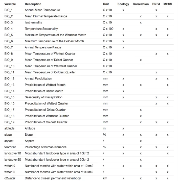
African occurrence data was acquired from the open-access Global Biodiversity Information Facility (GBIF.org) using the R package rgbif (Chamberlain et al., 2020). Only GBIF occurrences situated within the native range reported by Birdlife International (2020) were retained. European distribution data was likewise downloaded from GBIF and occurrences were filtered using the DAISIE inventory of alien

Figure 1. Left) Plot of all 90.067 native occurrences extracted from GBIF. Right) Plot of the remaining 422

native occurrences after rarefying with a distance of 50 km. Rarefying for the greatest part removed occurrences from intensively sampled areas such as South Africa and Kenya.

invasive species in Europe (Roy et al., 2020). South American occurrences were derived from Silva et

al. (2018), who made a selection based on ornithological collections, literature reviews and personal

field records. Typically, GBIF data shows a considerable amount of observer bias due to unequal sampling effort in different countries and regions (Beck et al., 2014). This oftentimes results in distorted distribution predictions and accuracy (Veloz, 2009; Yang et al., 2013). Spatial rarefying can reduce this spatial bias and generally leads to better predictions (Boria et al., 2014). All occurrences for Africa, Europe and South America were therefore rarefied using the R package humboldt (Brown & Carnaval, 2019) to obtain a minimum distance of 50km between all presence points. As a result, occurrences were reduced from 90.067 to 422, from 953 to 65 and from 573 to 200 points respectively for Africa, Europe and South (Figure 1).

3.2.3. Explanatory variables

Twenty-eight different variables were integrated for model construction (Table 2). Predictors were chosen to cover all categories proposed by Guissan & Thuiller (2005). First of all, climatological data was integrated from the Worldclim database by using nineteen variables representing temperature and precipitation (Hijmans et al., 2005). Secondly, three topographic parameters - altitude, slope and aspect - were incorporated in the model as well (Hijmans et al., 2005). Next, the Global Human Footprint Index developed by WCS (2005) was included, representing the percentage of human influence in an area. This map was built on information about population density, infrastructure and accessibility to humans. All mentioned predictors were downloaded on a 1x1 km2 _{resolution and scaled}

up to a 10x10 km2 _{resolution by averaging, using the raster package (Hijmans et al., 2014).}

Further, land cover and water availability were incorporated as resource factors. Land cover data was obtained from the ESA Climate Change Initiative providing land use data on a 300x300 m2 _resolution

(Defourny, 2016). Upscaling to a 10x10 km2 _{scale was achieved by aggregating and selecting the most}

common land cover type in the area. Secondly, surface water data was derived from the European Commission Climate databases (Pekel et al., 2016). This fine-grained map on a scale of 30x30 m2

provides information about the average number of months per year surface water is present in the area. For water availability, upscaling to 10x10 km2 _{was achieved by selecting the maximum number}

of months per area.

Land cover and water availability were also taken into account in the wider area of 30km. Common waxbills are mostly sedentary, but occasionally wander locally. Ringed birds were frequently recaptured outside their nest range, mostly within a distance of 30 km of the ringing place (Fry et al., 2004). Upscaling to 30 km was done by creating a circular moving window with a radius of 30km using the R package raster (Hijmans et al., 2014) and likewise selecting the most common - for land cover - or maximum - for water availability - value for aggregation. Finally, distance to the closest permanent surface water body was also calculated.

Table 2. Overview of all twenty-eight variables used as predictors. In the collumns “Ecology”, “Correlation”,

“ENFA” and “MESS”, the fifteen used predictors for the respective variable slections strategies are indicated. 3.2.4. Spatially blocked cross-validation

The baseline model was constructed based on a spatially blocked five-fold cross validation strategy. An obstacle in species distribution modelling is the inherent presence of spatial autocorrelation in both occurrences and predictor variables (Bahn & McGill, 2013; Hijmans, 2012). This indicates that testing points close to training points will not be independent and accordingly less informative for assessing model performance (Bahn & McGill, 2013). Spatially blocked cross-validation can provide a solution to make test and train data more independent (Roberts et al., 2017) and generally improves model transferability (Hao et al., 2020; Radosavljevic & Anderson, 2014).

In this approach, the native range was divided in spatial blocks that were alternatingly used for training and testing. First of all, optimal blocksize was determined by using the function spatialAutorange in the package BlockCV (Valavi et al., 2019). This function assesses the spatial autocorrelation within every predictor in the native range based on 100.000 sample points and reports the range over with each of these variables is independent (figure 2, variogram). As proposed by Valavi et al. (2019), the median distance of all included predictors was chosen as block size. The optimal block size was calculated separately for every variable selection strategy, in order to make the effect of spatial autocorrelation equal in every approach. Subsequently, the native range was divided in spatial blocks based on the previously determined block size and each block was randomly assigned to one of the five folds in our 5-fold cross-validation strategy (figure 2, map). Final blocks were chosen through a 1000fold iteration to make sure the number of presences and absences were well-balances over all folds. Finally, cross-validation was performed by alternatingly selecting blocks from 4 folds to train the model and using the remaining block to extract test data.

3.2.5. Model evaluation

Models were evaluated using the True skill statistic (TSS). This statistic equals the sum of the proportion of occurrences that are correctly classified - sensitivity - and the proportion of correctly classified absences - specificity - minus one (Allouche et al., 2006). TSS is a threshold dependent value, since it needs a cut-off value to classify continuous habitat suitability values as presences or absences. An adjusted function of the R package ecospat (Di Cola et al., 2016) was used to calculate the TSS value for all thresholds from 0.01 to 0.99 and select the threshold that maximizes TSS (maxTSS). Sensitivity

ddd

Figure 2. Left) Variogram depicting the range over which each variable is independent (example of the fifteen

variables included in the ENFA-based strategy). The red dotted line indicates the median value over all variables and was used as block size. Right) Example of spatial blocks, each of them randomly assigned to one of the five

and specificity values were also evaluated separately, since both provide a more detailed insight in prediction accuracy (Jiménez-Valverde et al., 2011). MaxTSS, sensitivity and specificity values were calculated based on a 100fold iteration using the rarefied presence data and randomly selected pseudo-absences.

3.2.6. Environmental similarity

To assess the reliability of model predictions in the invasive range, multivariate environmental similarity surface analysis maps were calculated for the baseline model (MESS; Elith et al., 2010). This method compares a reference area - the native range - with a new area - the invasive range - and calculates the environmental similarity between both. For every 10x10 km2 _{grid cell in the European}

and South American continent, the ecological similarity with the environmental conditions available in the native range was compared. Cells with negative similarity values indicate unprecedented ecological conditions, implying that prediction in these grids are the result of extrapolation and should therefore be interpreted with caution (Elith et al., 2010). In addition, the most influential variables contributing to environmental dissimilarities were also investigate using the MoD function in the package modEvA (Barbosa et al., 2015).

3.3. Variable selection strategies

To investigate the effect of a priori predictor choice, five strategies of variable selection were tested by example of Petitpierre et al. (2017). In the first strategy, all 28 predictors were included in the model. In all four alternative strategies, a selection of 15 explanatory variables was made. An overview of the selected predictors in every strategy can be found in Table 2.

3.3.1. Ecology based

For the first variable strategy, the fifteen most ecologically important predictors were selected. First, climatological variables were incorporated since they often determine the broad patterns of occurrence (Pearson & Dawson, 2003). For both temperature and precipitation, variables representing annual mean values, seasonality and maximum and minimum values were chosen. Secondly, the common waxbill is strongly bound to water and is often found at the banks of streams, lakes and ponds (Fry et al., 2004). Distance to permanent water and duration of surface water in the surrounding area of 10x10 km2 _{were consequently chosen as predictors. Thirdly, Estrilda astrild is a granivorous bird,}

typically feeding on small grass seeds. Accordingly, it is tied to grass lands, cereal fields or low herb vegetation (Fry et al., 2004). Land cover was therefore integrated as a crucial ecological factor. Since individuals can regularly be found in presence of humans, the Human Footprint Index was also included (Fry et al., 2004). Finally, the topographic variables altitude and slope were incorporated as well.

3.3.2. Correlation based

Multicollinearity can reduce prediction success of species distribution models (Braunisch et al., 2013). In this case, the probability of creating statistically substantiated but ecologically meaningless relationships with an intercorrelated predictor increases. These spurious correlations will most likely

not hold in new environments, affecting the transferability of the model (Dormann et al., 2008). Analogous with Petitpierre et al. (2017), pairwise Pearson correlation coefficients were calculated between all variables. From al predictor pairs with a correlation coefficient higher than 0.6, the least ecologically meaningful variable was eliminated (Austin, 2007).

3.3.3. ENFA – Ecological niche factor analysis

Next, an ecological niche factor analysis was used to achieve a more data-driven approach to variables selection. The ENFA framework created by Hirzel et al. (2002) assesses the probable contribution of each explanatory variable to the distribution of the species and was performed using the package CENFA (Rinnan, 2020). Since this method cannot handle extensively high correlation between parameters, three highly correlated predictors (BIO_9, BIO_17, BIO_18) were removed for the analysis. In this case, the aim of the ENFA analysis was to obtain two parameters for every variable: the marginality factor and the specialization factor (Lobo et al., 2010). The marginality factor represents the distance between the optimal ecological space the common waxbill occupies and the mean ecological space available in the Afrotropical region. The specialization factor equals the ratio of variance in the whole Afrotropical region and that of the common waxbill’s ecological space (Basille et

al., 2008). The fifteen variables with the highest combined sum of the marginality and specialization

factor were eventually selected (Lobo et al., 2010).

3.3.4. MESS – Multivariate Environmental Similarity Surface

As a final variable selection strategy, predictors were chosen based on a multivariate environmental similarity surface analysis (MESS; Elith et al., 2010, see section 3.2.6). The MESS function in the R package modEVA (Barbosa et al., 2015) was adjusted in order to compare individual predictors between the native and invasive ranges. Similarity values for each variable were calculated between both the Afrotropical region and Europe and the Afrotropical region and South America. Finally, the fifteen predictors with the highest combined sum of the similarity values were used for this variable selection strategy.

3.4. Background selection

To investigate the effect of a priori background choice, four distinct strategies of background selection were assessed. All models were created with neutral prevalence for presences and pseudo-absences (Barbet-Masin et al., 2010; Senay et al., 2013).

3.4.1. Zoogeographical region

As a first background selection strategy, all pseudo-absences were randomly chosen within the Afrotropical zoogeographical region. The outlines of zoogeographical regions correspond to influential boundaries delaminating the range of multiple species (Barve et al., 2011). Complying with the full native range of the common waxbill, the Afrotropical region theoretically represents the geographical area the species was able to sample. By selecting pseudo-absences in the zoogeographical region, the distance between pseudo-absences and presences was not too large and overprediction was avoided

(VanderWal et al., 2009). All three following strategies were framed within this Afrotropical zoogeographic region as well.

3.4.2. Buffered presences

Not only the outer boundaries of the background area matter, pseudo-absences must also not be selected too close to presences in order to prevent losing coarse-scaled information (Sanchez-Fernandez et al., 2011). Following Barve et al. (2011), presences were buffered at a distance of 25, 50 and 75 km. This implicated that pseudo-absences could not be chosen closer than respectively 25, 50 and 75 km to presence points. Similar to the first strategy, further pseudo-absences selection also happened within the Afrotropical region.

3.4.3. Predefined probability of absence

Optimally, presence-only distribution models should select pseudo-absences that represent environmentally driven absences (Lobo et al., 2010). Pseudo-absences were therefore selected based on a predefined probability of absence. For all raster cells in the Afrotropical zoogeographical area, the environmental distance to the species’ range was calculated following Vilela (2017). Specifically, the ecological distance to all common waxbill occurrences was calculated and averaged for every raster in the Afrotropical region. Pseudo-absences were then chosen in such manner that ecologically more distant background cells had a higher chance to be selected as pseudo-absence (Lobo et al., 2010).

3.4.4. Target group approach

Sampling bias is ubiquitous in data provided by portals like GBIF and can severely distort prediction accuracy (Syfert et al., 2013; Yang et al., 2013). The African common waxbill dataset indeed contains clear sampling bias. For example, the South African Bird Atlas Project monitors the avifauna on a scale of 10x10 km2 _{grids, while other countries are strongly undersampled. The same pattern of sampling}

effort can be seen in GBIF records for all Passeriformes (Figure 3). One way to account for this sampling Figure 3. GBIF occurrences in Africa for the common waxbill (left) and for all passerines (right). In both cases,

bias, is subjecting pseudo-absences to the same bias as presences using a so-called target group approach (Hertzog et al., 2014; Phillips et al., 2009). In this framework, occurrences of a particular target group inform the selection of pseudo-absence data. Here, all passerine occurrences for the Afrotropical region were downloaded from GBIF and selected as target group (GBIF.org). Pseudo-absences were then only extracted from grid cells containing sightings for other Passeriformes.

3.5. Subspecific niche variation

3.5.1. Morphological differentiation

3.5.1.1. Museum measurements

To asses subspecific differentiation within the Common waxbill, morphological measurements were taken on museum specimens from the Royal Belgian Institute of Natural Sciences and the Royal Museum for Central Africa. First of all, all available specimens were identified to subspecies level and georeferenced using the R package dismo (Hijmans et al., 2017). The most intact and least distorted specimen for every unique location with a coordinate uncertainty lower than 50 km was chosen. This resulted in a selection of 120 specimens from 8 different subspecies. Secondly, a set of 32 morphological traits reflecting niche characteristics was measured on every specimen (Kearney et al., 2010). To reduce measuring inaccuracies, all measurements were performed twice and values were averaged. The 32 measurements consisted of both allometric features and feather characteristics. Allometric measurements included the distal orientation, length and proximal orientation of the head, neck, torso, tarsus and beak. In addition, tail length, and full body length were assessed as well. Secondly, dorsal and ventral feather depth and length of the head, neck and torso feathers were chosen as feather characteristics.

3.5.1.2. Morphometric analysis

First of all, a linear discriminant analysis (LDA) was performed to visualize morphological difference between subspecies (Venables & Ripley, 2002). This technique aims to optimize discrimination between subspecies by minimizing the within-group variance and maximizing the variance between groups. Typically, LDA algorithms are unreliable when the number of specimens is significantly smaller than the number of variables (Fukunaga, 1990). Subspecies that were represented by less than 10 specimens – minor and astrild – were therefore removed for analysis. Finally, the resulting dataset contained 100 specimens from 6 different subspecies. Since outcomes of linear discriminant analyses can be distorted by multicollinearity (Naes & Mevik, 2001), a scaled principal component analysis was executed beforehand. LDA was then performed directly on the PCA scores (Yang & Yang, 2003). Secondly, detection of statistical morphological differences between subspecies was achieved by executing a Permutational multivariate analysis of variance based on 100.000 permutations and Mahalanobis distance (PERMANOVA; Anderson, 2001). Significance of pairwise differences were subsequently assessed in a post-hoc analysis by using the pairwise.adonis package (Martinez, 2020). Respective p-values were adjusted by Bonferroni correction.

3.5.2. Subspecific Occurrences

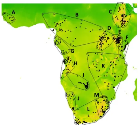
In order to perform further niche analyses and create subspecific models, subspecies-level occurrence data was gathered. First, subspecies-level occurrences were extracted from GBIF using the R package rgbif (Chamberlain et al, 2020). Locations without coordinates were georeferenced and the uncertainty on the coordinates was calculated. The subspecies angolensis and jagoensis were lumped since they almost completely overlap in range. Based on descriptions from Fry et al. (2004), the accuracy and authenticity of every occurrence was verified. Subsequently, the GBIF data was combined with earlier georeferenced museum specimens. Presences with a location uncertainty greater than 50 km were removed from the dataset. In the remaining dataset, still more than half of the subspecies contained less than 15 occurrences. The minimum number of occurrences needed to create trustworthy distribution models ranges from 15 (Papes & Gaubert, 2007) to 20 (Stockwell & Peterson, 2002) to 45 (van Proosdij et al., 2016). Therefore, minimum convex polygons were drawn around all subspecific occurrences using R package rgeos (Bivand & Rundel, 2012; Figure 4). Non-overlapping polygons were used to subtract species-level occurrences from GBIF and these occurrences were assigned to the respective subspecies. Lastly, all occurrences were rarefied at a distance of 10 km, so that every occurrence represented a separate raster cell in the model (Table 3).

3.5.3. Niche differentiation

To investigate possible niche variation between subspecies, pairwise comparisons of niche space were performed using the R package ecospat (Di Cola et al., 2016) following the framework of Broenniman

et al. (2012). Prior to the niche analysis, a principal component analysis of the twenty-eight predictor

variables was performed for the full zoogeographical region and the subspecies ranges separately. The first and second principal components were used to create the ecological space to perform all niche calculations. First of all, niche overlap between all thirteen subspecies in this two-dimensional PCA space was calculated based on Schoener’s D (Schoener, 1982). This value varies between 0 and 1 and represents the proportion of overlap between the niche of two subspecies, corrected by availability of background conditions in the Afrotropical zoogeographic region. Afterwards, pairwise niche similarity tests were performed to investigate if the ecological niche of any pair of subspecies was more different than expected by chance (Warren et al., 2008).

3.5.4. Subspecific model implementation

Both the morphometric and niche analysis discovered differences in niche characteristics between subspecies (see results below). Species distribution models on subspecies level were therefore constructed to assess the effect of within-taxon niche differentiation on model predictions. The three best performing parametrization strategies for predicting the African range (see Table 1) were built again for each of the thirteen subspecies separately (Table 3). Final habitat suitability maps for Africa, Europe and South America were obtained by combining all predictions of subspecific models and taking the maximum value in each grid cell, by example of Schulte et al. (2011).

Table 3. Final number of occurrences

per subspecies used for niche analysis and subspecific model building.

Figure 4. Map of the polygons delineating the occurrences of the

subspecies. The subspecies are: A) kempi B) occidentalis C) peasei D) adesma E) massaica F) minor G) rubriventris H) jagang: fusion of jagoensis and angolensis I) niediecki J) damarensis K) cavendishi L)

4. RESULTS

4.1. Overall prediction success

As regards maxTSS for the native predictions, all 30 model variants perform relatively well. MaxTSS values are altogether fairly similar and range from 0.705 to a maximum of 0.758 (Table 4). Similarly, maxTSS scores for the South American predictions are also comparable between all model variants. Forecasting accuracy is however overall low with values ranging from 0.281 to 0.356. MaxTSS scores for the European predictions fluctuate more pronouncedly and values go from -0.013 up until 0.716. Overall, values are rather low with only 5 of the 30 model variants displaying a value over 0.4.

As to the sensitivity of all model predictions, different patterns can be distinguished. For the native and South American range, differences in maxTSS are seemingly randomly driven by both specificity and sensitivity. Improvements in model predictions are occasionally related to a higher amount of correctly classified presences, other times to correctly classified absences. For the European predictions however, improvements in maxTSS values are mostly related to increases in sensitivity and not in specificity, indicating that model accuracy is in this case predominantly driven by correct detection of presences.

Table 4. Evaluation statistics maxTSS (TSS) and sensitivity (Sens) for all 30 variations of the species-level model.

Interestingly, model variants with a higher maxTSS score for predictions in the native range do not automatically better predict the European or South American range. Correlation coefficients were calculated between the maxTSS values for Africa, Europe and South America. Africa and Europe and Africa and South America showed a correlation of respectively -0.189 and -0.097, indicating no distinct trend between prediction success of the native and invasive range. Moreover, the model with the highest maxTSS value for Europe was the 3th _{worst performing model in the native range. The 8}th _worst

performing model concerning the African range resulted in the highest maxTSS value for the South American range.

4.2. Effect of variable selection

Figure 5. Average maxTSS values for A) Africa B) Europe C) South America for all five variable selection strategies:

All, Correlation, Ecology, ENFA and MESS. Blue bars indicate the average for every variable selection strategy, black flags mark the standard deviation around the mean.

For the native and South American range predictions, no clear difference in prediction accuracy can be observed between the five variable selection strategies (Figure 5A & 5C). There is no observable disparity neither between nor within particular variable selection strategies. For Europe however, clear differences between the strategies can be noticed. Models with variables selected based on correlation and MESS results (“Corr” and “MESS”; Figure 5B), are clearly inadequate when predicting the European invasive range. Both display a mean maxTSS value close to zero and all models within these strategies perform equally bad. Model strategies “Eco” and “ENFA” perform best, although standard deviation for both strategies are relatively high. For the ENFA based variable selection, this high standard deviation is the result of one particular, badly performing model with a maxTSS value of 0.066 (Table

4). All other models perform relatively well. For the ecology-based variable selection, maxTSS statistics

fluctuate more between different models and range from 0.066 to 0.661.

4.3. Effect of background selection

Models could not be constructed for the target group approach, since none of the underlying, individual models for ensemble building showed a TSS value above 0.7. For all other background selection strategies, ensemble models could be constructed. Similar to the result concerning variable selection, all background selection strategies perform equally well when predicting the native and

South American range (Figure 6). MaxTSS values in all background selections fluctuate around 0.75 and 0.3 for respectively the native and South American range. By contrast, slight differences between the five background strategies can be noticed when forecasting the European distribution. Background selections based on the zoogeographical region (“Zoogeo”) and predefined probabilities of absence (“Prob”) show a slightly higher mean maxTSS. However, standard deviations are too high to conclude actual difference between background strategies. The high standard deviations for all groups are most likely driven by variable selection, since the respective “ENFA” and “Eco” strategies consistently outperform the other variable selection strategies within all strategies of background selection.

Figure 6. Average maxTSS values for A) Africa B) Europe C) South America for all five background selection

strategies: Buffer25, Buffer50, Buffer75, Probability of Absence and Zoogeographical region. Blue bars indicate the average over the background selection strategy, black flags indicate the standard deviation.

4.4. Accounting for subspecific niche variation

4.4.1. Assessment of subspecific differentiation

Results of the LDA analysis hint at differences in morphological traits between certain subspecies (Figure 7). Particular subspecies such as rubriventris and peasei are relatively well separated in the morphological space. Results of the PERMANOVA statistically substantiate these graphical indications (p=0.006). Post-hoc analysis discovered significant differences in morphological characteristics in three out the fifteen subspecies combinations; between peasei and rubriventris (p=0.015), between

occidentalis and rubriventris (p=0.030) and between adesma and rubriventris (p=0.050).

Aside from differences in morphology, analysis of niche space also clearly indicates niche differentiation between multiple subspecies. Following the outcomes of the niche similarity test, the ecological niche of 84 of the 87 subspecies combinations was not more similar than expected by chance (p > 0.05; table 5). Only three subspecies pairs (tenebridorsa-astrild, tenebridorsa-cavendishi and

Figure 7. Biplot of the linear discriminant analysis based on the morphological dataset of 100 specimens out

of 6 subspecies. LDA1 and LDA2 explain respectively 32.6% and 26.6% of between-group variation.

4.4.2. Effect of incorporating subspecies

As regards the prediction for the native African range, subspecies-level models consistently show higher maxTSS values than the corresponding species-level model strategies, with an average increase of 0.058 (Table 6). This improvement seems to be driven by a higher proportion of correctly classified absences, since all model predictions show a higher specificity. For the European predictions, two out of tree subspecies-level models have a slightly lower maxTSS value compared to the species model. Both models show an increase in sensitivity and a decrease in specificity. The subspecies-level model 3.1 however, performs clearly worse than its species-level equivalent. The ability to correctly detect

Table 5. Table with p-values for the pairwise niche similarity tests for all subspecies combinations. Blue

presences drops drastically, while it better detects absences. As to predictions for the South American range, two out of the three subspecies-level models show a slight increase in maxTSS compared to the species-level model. While for model 2.1.1 the sensitivity clearly increases, the specificity of model 3.3 decreases. MaxTSS decreases for subspecies-level model 3.1, coinciding with a drop in specificity.

Figure 8. Habitat suitability maps created for the best performing model variant in the native range

(Model 2.1.1). A, C and D represent the habitat suitability maps for the species-level modelling approach. B, D and F represent the habitat suitability maps for the subspecies-level modelling

approach. Suitability ranges from 0 (unsuitable, pink) to 1 (very suitable, dark green).

Table 6. maxTSS (TSS), sensitivity (Sens) and specificity (Spec) values for predictions of the native, European and

South American ranges for the three model variants performed both on species and subspecies level. The blue columns indicate values for the species-level variant, the white columns for the subspecies-level variant.

4.5. Environmental similarity

For the European predictions, extrapolation happens in 78.1% of all grid cells (Figure 9). The majority of the remaining locations are classified as marginal habitat (18.8%), while only 3.1% of grid cells represent environmental conditions similar to the Afrotropical region. The mean MESS value of all grid cells with a positive similarity value equals 0.03, implying environmental conditions with still a relatively low similarity to the Afrotropical region. BIO_4 (temperature seasonality), BIO_11 (mean temperature of the coldest month) and BIO_8 (mean temperature of the wettest quarter) are the main contributors to dissimilarity with the native range in respectively 85.5%, 7.4% and 3.2% of the cases. In the South American range, 13.8% of all grid cells show a negative MESS similarity value, indicating that models need to extrapolate when predicting to these locations (Figure 9). The great majority of locations (67.0%) shows a MESS value of 0, pointing at marginal habitat. Only 19.2% of the total South American continent consists of environmental condition similar to those is the Afrotropical region. The mean MESS value of all grid cells with a positive similarity value equals 3.58. The most important variables contributing to dissimilarity with the native range are BIO_14 (precipitation of the driest month: 26.11% of grids), BIO_8 (mean temperature of the wettest quarter: 22.81% of grids) and BIO_17 (precipitation during the driest quarter: 16.84% of grids).

Figure 9. Multivariate environmental surface maps for both Europe (left) and South America (right).

Orange colored locations indicate negative similarity values. These are locations where extrapolation happens when predicting habitat suitability. Yellow colored locations mark grid cells with a MESS value of 0, referred to as “marginal habitat”. This habitat is not unprecedented in the native range, but represents environmental conditions that are extremely rare in the native range. Green locations have positive MESS value, meaning these locations are environmentally similar to those present in the native range.

4.6. Variable importance

The five overall most important variables for the three species-level model strategies yielding the best prediction for the native (Model 2.1.1, Model 3.1, Model 3.3; Table 1), European (Model 1.4, Model 3.2, Model 2.4.1) and South American range (Model 1.5, Model 1.4 and Model 1.1) are depicted in Table 5. The variables BIO_11 (mean temperature of the coldest quarter) and BIO_5 (maximum temperature of the warmest month) are among the most important variables for all three ranges. In two of three geographical ranges, BIO_2 (mean diurnal temperature range) and BIO_12 (annual precipitation) appear among the most important

predictors. Furthermore, minimum temperature of the coldest month (BIO_6) and the annual temperate range (BIO_7) are influential variables for correctly predicting the native range, while the annual mean temperature (BIO_1) and water availability in the area of 10x10 km2 _{(water10) are}

important in constructing the most accurate European predictions. Finally, BIO_2 (annual precipitation) and BIO_4 (temperature seasonality) came up as leading variables in the best performing models for predicting the South American range.

Table 7. Overall most important variables for

the three best performing models in the native, European and South American range.

5. DISCUSSION

5.1. Overall species-level model accuracy

All species-level models constructed in this study perform relatively well when intrapolating across the native range (Figure 10). MaxTSS values for the African range predictions are all higher than 0.7, a regularly used cut-off value to classify predictions as accurate (Thuiller et al., 2013). This indicates that all species-level models sufficiently capture the relations driving the distribution of common waxbills in their native range. On the contrary, none of the species-level model variants is able to accurately predict the invasive range of the Common waxbill, neither in South America nor in Europe. Following the overall prediction trends from our study, suitable habitat for the Common waxbill is present in all climate types of the South American continent, except for the tropical monsoon, savannah and rainforest areas [based on the Köppen-Geiger climate classification (Beck et al., 2018)]. Suitable areas include the whole West Coast of South America, Patagonia and the temperate regions of south-eastern Brazil (Figure 10). However, physiological information derived from captive waxbills indicates a strong sensitivity to temperatures below 15°C (Nicolai & Steinbacher, 2002), making it very unlikely for the common waxbill to ever establish viable populations in areas such as the Andes mountains or Patagonia. Although our models overpredict in these colder regions, underprediction also occurs. The whole Amazon basin is considered unsuitable following our species-level predictions, while da Silva et

al. (2018) reported occurrences in this area.

Most species-level model variants are also unable to correctly predict the European range. Predicted habitat suitability varies between 0.614 and 0.926, making the whole continent of Europe suitable for the common waxbill (Figure 10), from the Mediterranean climates in Spain up until freezing conditions above the North Pole circle. Similar to South America, these habitat suitability maps do not realistically reflect the potential invasive distribution of the common waxbill in Europe as models are obviously Figure 10. Habitat suitability maps for Africa, Europe and South America based on the best performing

species-level model variant in the native range (Model 2.1.1). Suitability ranges from 0 (unsuitable, pink) to 1 (very suitable, dark green). On every map, rarefied occurrences used to test the model are plotted.

overpredicting. These results are not surprising, since the lack of transferability from models performing well in the native range has been reported multiple times already (Beaumont et al., 2009; Fitzpatrick et al., 2007; Randin et al., 2006).

5.1.1. Transferability to non-analogue climates

The overall low accuracy of both the European and South American range predictions could be the result of strong environmental dissimilarity between the three continents. Overall, environmental conditions strongly differ between Africa, South America and Europe. Results from the MESS analysis indicate that only respectively 3.1% and 19.2% of grid cells in Europe and South America are environmentally similar to the Afrotropical region. This is a low percentage, considering the often-mentioned problems of SDM transferability to non-analogues climates (Guisan et al., 2014; Harisson

et al., 2006; Rodríguez‐Castañeda et al., 2012).

Low predictive accuracy when extrapolating SDMs to non-analogue conditions can have multiple causes. First of all, the native niche space in which SDMs are trained can be truncated due to unavailability of more extreme conditions for certain predictors (Williams & Jackson, 2007). In this case, one or multiple response curves are cut off at a certain value and model predictions behind these values are uncertain. When predicting to non-analogues climates, extrapolating truncated response curves can result in both over- and underestimation of the invasive range (Hanneman et al., 2015). Secondly, the correlation structure among predictor variables in non-analogues locations can also be different compared to the native area (Heikkinen et al., 2006; Peterson, 2011). For example, SDMs can pick up statistically substantiated but ecologically meaningless relationships with indirect predictors, driven by an underlying correlation with direct predictors. When projecting these relations to areas with a different correlation structure, the relations with the indirect predictor will become indiscriminative in the novel area. Extrapolation of SDMs to dissimilar ecoclimatological conditions can therefore lead to unreliable predictions (Dormann et al., 2008; Elith & Leathwick, 2009; Guisan et al., 2014).

Since percentages of environmental similarity are so low between Africa, Europe and South America, the problem of transferability to non-analogues climates is most likely a driver behind the low model transferability and resulting inaccurate predictions found in this study. For Europe, models need to extrapolate to unknown conditions in 78.1% of the time and this could possibly result in the drastic overprediction observed in this study. Similar for South America, 13.8% of grid cells require extrapolation. Large parts of these dissimilar regions consist of the Andes Mountains and parts of the Amazon basin of north-West Brazil, Southern Colombia and Northern Peru (Figure 9). These environmentally dissimilar locations indeed coincide with locations were the species-level models both over- and underpredict for South-America.

5.1.2. Restrictive SDM assumptions

The overall low performance of species-level models caused by both over- and underprediction of the invasive range, could also partially be the result of the assumptions underlying SDMs. First of all, underprediction could arise out of violations on the assumptions of niche equilibrium and niche

conservatism. SDMs assume that a species is in equilibrium with its environment, meaning that it fully occupies all suitable locations in the native range (Guissan & Thuiller, 2015). The niche space based on native occurrences should then ideally capture the full fundamental niche. This assumption implies that neither biotic interactions nor dispersal limitations influence the species’ distribution. In reality, the environmental niche space captured by SDMs most likely reflects the realized niche instead of the fundamental niche (Broenniman et al., 2012; Guisan et al., 2012). Further, species are expected to conserve their niche during invasion (Araujo & Peterson, 2012; Wiens & Graham, 2005). Following this assumption of niche conservatism, species can only invade geographical areas characterized by parameter values inside the native niche. In its native range, the common waxbill shows distributional gaps in the tropical forest of the Congo basin (Figure 11; Billerman et al., 2020). As a consequence, models predict very low habitat suitability for waxbills in the tropical Amazon basin. However, the common waxbill is spreading into the Amazon basin according to multiple sources (GBIF.org; Silva et

al., 2018). Niche analyses by Silva et al. (2018) also described an expansion of the native niche into

tropical South America. This could reflect an actual niche shift, where the fundamental niche of the common waxbill has broadened after introduction (Broenniman et al., 2007; Petitpierre et al., 2012). However, this could also imply that models build on the native range are failing to capture the complete fundamental niche of the common waxbill (Peterson, 2011). Underprediction in the Amazon region could therefore possibly result from deviations of the assumption of niche conservatism or equilibrium. Further, overprediction of invasion risk may be attributed to the species’ invasions history (Gallien et

al., 2012), as the common waxbill was introduced in Europe and South America during the 19th _century

(Sick, 1997). Most likely, the species may not yet be in equilibrium with its environment in the invasive ranges (Guissan & Thuiller, 2015). Further spread of the common waxbill in Europe and South America is still possible as waxbills likely have not had sufficient time to colonize all suitable areas that are present. However, none of the eco-evolutionary processes such as niche shifts, invasion history and dispersal limitations can explain why SDMs mark parts of Europe and South-America that are clearly much colder than the native range as suitable. Such obvious overprediction is likely attributable to SDM methodological assumptions and limitations as explained above.